10 MB pdf-file here - NTNU
10 MB pdf-file here - NTNU
10 MB pdf-file here - NTNU

Create successful ePaper yourself
Turn your PDF publications into a flip-book with our unique Google optimized e-Paper software.
Contents<br />
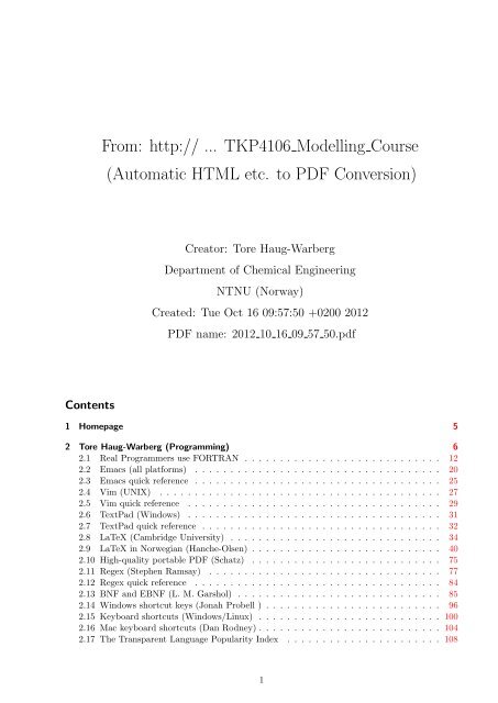
From: http:// ... TKP4<strong>10</strong>6 Modelling Course<br />
(Automatic HTML etc. to PDF Conversion)<br />
Creator: Tore Haug-Warberg<br />
Department of Chemical Engineering<br />
<strong>NTNU</strong> (Norway)<br />
Created: Tue Oct 16 09:57:50 +0200 2012<br />
PDF name: 2012 <strong>10</strong> 16 09 57 50.<strong>pdf</strong><br />
1 Homepage 5<br />
2 Tore Haug-Warberg (Programming) 6<br />
2.1 Real Programmers use FORTRAN . . . . . . . . . . . . . . . . . . . . . . . . . . . . 12<br />
2.2 Emacs (all platforms) . . . . . . . . . . . . . . . . . . . . . . . . . . . . . . . . . . . 20<br />
2.3 Emacs quick reference . . . . . . . . . . . . . . . . . . . . . . . . . . . . . . . . . . . 25<br />
2.4 Vim (UNIX) . . . . . . . . . . . . . . . . . . . . . . . . . . . . . . . . . . . . . . . . 27<br />
2.5 Vim quick reference . . . . . . . . . . . . . . . . . . . . . . . . . . . . . . . . . . . . 29<br />
2.6 TextPad (Windows) . . . . . . . . . . . . . . . . . . . . . . . . . . . . . . . . . . . . 31<br />
2.7 TextPad quick reference . . . . . . . . . . . . . . . . . . . . . . . . . . . . . . . . . . 32<br />
2.8 LaTeX (Cambridge University) . . . . . . . . . . . . . . . . . . . . . . . . . . . . . . 34<br />
2.9 LaTeX in Norwegian (Hanche-Olsen) . . . . . . . . . . . . . . . . . . . . . . . . . . . 40<br />
2.<strong>10</strong> High-quality portable PDF (Schatz) . . . . . . . . . . . . . . . . . . . . . . . . . . . 75<br />
2.11 Regex (Stephen Ramsay) . . . . . . . . . . . . . . . . . . . . . . . . . . . . . . . . . 77<br />
2.12 Regex quick reference . . . . . . . . . . . . . . . . . . . . . . . . . . . . . . . . . . . 84<br />
2.13 BNF and EBNF (L. M. Garshol) . . . . . . . . . . . . . . . . . . . . . . . . . . . . . 85<br />
2.14 Windows shortcut keys (Jonah Probell ) . . . . . . . . . . . . . . . . . . . . . . . . . 96<br />
2.15 Keyboard shortcuts (Windows/Linux) . . . . . . . . . . . . . . . . . . . . . . . . . . <strong>10</strong>0<br />
2.16 Mac keyboard shortcuts (Dan Rodney) . . . . . . . . . . . . . . . . . . . . . . . . . . <strong>10</strong>4<br />
2.17 The Transparent Language Popularity Index . . . . . . . . . . . . . . . . . . . . . . <strong>10</strong>8<br />
1
2.18 The Hows and Whys of Commenting (C) . . . . . . . . . . . . . . . . . . . . . . . . 116<br />
2.19 99 bottles of beer (<strong>10</strong>00++ languages) . . . . . . . . . . . . . . . . . . . . . . . . . . 119<br />
2.20 Programming paradigms (Kurt Normark) . . . . . . . . . . . . . . . . . . . . . . . . 120<br />
2.21 Real Programmers (Ed Post), see also Sec. 2.1 . . . . . . . . . . . . . . . . . . . . . 126<br />
2.22 The story of Mel (Ed Nather,) . . . . . . . . . . . . . . . . . . . . . . . . . . . . . . 127<br />
2.23 The Tao of programming (Kragen Sitaker) . . . . . . . . . . . . . . . . . . . . . . . . 133<br />
2.24 Computer languages (E. Levenez) . . . . . . . . . . . . . . . . . . . . . . . . . . . . . 148<br />
2.25 Shoot yourself in the foot (WWW) . . . . . . . . . . . . . . . . . . . . . . . . . . . . 155<br />
2.26 Lord of the Rings (D. Pritchard) . . . . . . . . . . . . . . . . . . . . . . . . . . . . . 159<br />
2.27 About spell checkers (WWW) . . . . . . . . . . . . . . . . . . . . . . . . . . . . . . . 161<br />
2.28 Foobar etymology (Jargon File) . . . . . . . . . . . . . . . . . . . . . . . . . . . . . . 163<br />
2.29 2000 languages . . . . . . . . . . . . . . . . . . . . . . . . . . . . . . . . . . . . . . . 165<br />
2.30 A Beginner’s Python Tutorial (Steven Thurlow) . . . . . . . . . . . . . . . . . . . . . 191<br />
2.31 Epytext markup (sourceforge) . . . . . . . . . . . . . . . . . . . . . . . . . . . . . . . 193<br />
2.32 Epydoc fields (sourceforge) . . . . . . . . . . . . . . . . . . . . . . . . . . . . . . . . 203<br />
2.33 Python Docstrings (Sourceforge) . . . . . . . . . . . . . . . . . . . . . . . . . . . . . 211<br />
2.34 Regex in Python (McCormack) . . . . . . . . . . . . . . . . . . . . . . . . . . . . . . 213<br />
2.35 Unit Testing in Python (William Blum) . . . . . . . . . . . . . . . . . . . . . . . . . 226<br />
2.36 Python best practise (Well House) . . . . . . . . . . . . . . . . . . . . . . . . . . . . 230<br />
2.37 Numerical Python (scipy.org) . . . . . . . . . . . . . . . . . . . . . . . . . . . . . . . 246<br />
2.38 Plotting with Python (matplotlib) . . . . . . . . . . . . . . . . . . . . . . . . . . . . 247<br />
2.39 Scientific Python (scipy.org), see also Sec. 2.37 . . . . . . . . . . . . . . . . . . . . . 251<br />
2.40 Symbolic Python (sympy.org) . . . . . . . . . . . . . . . . . . . . . . . . . . . . . . . 252<br />
2.41 Functional Python (Moka) . . . . . . . . . . . . . . . . . . . . . . . . . . . . . . . . . 254<br />
2.42 The Transparent Language Popularity Index, see also Sec. 2.17 . . . . . . . . . . . . 264<br />
3 Heinz A. Preisig (Modelling) 265<br />
4 Frequently Asked Questions (FAQ) 266<br />
4.1 use epydoc . . . . . . . . . . . . . . . . . . . . . . . . . . . . . . . . . . . . . . . . . 269<br />
5 Syllabus 275<br />
5.1 Getting started . . . . . . . . . . . . . . . . . . . . . . . . . . . . . . . . . . . . . . . 276<br />
5.1.1 Ken Olsen, founder of DEC (1977) . . . . . . . . . . . . . . . . . . . . . . . . 280<br />
5.1.2 A Smalltalk about Modelling . . . . . . . . . . . . . . . . . . . . . . . . . . . 282<br />
5.1.3 Regular Expressions, see also Sec. 2.11 . . . . . . . . . . . . . . . . . . . . . . 287<br />
5.2 Topology . . . . . . . . . . . . . . . . . . . . . . . . . . . . . . . . . . . . . . . . . . 288<br />
5.2.1 Reference ??? . . . . . . . . . . . . . . . . . . . . . . . . . . . . . . . . . . . . 290<br />
5.3 Documentation . . . . . . . . . . . . . . . . . . . . . . . . . . . . . . . . . . . . . . . 292<br />
5.3.1 The real programmer, see also Sec. 2.1 . . . . . . . . . . . . . . . . . . . . . . 296<br />
5.3.2 epydoc . . . . . . . . . . . . . . . . . . . . . . . . . . . . . . . . . . . . . . . . 297<br />
5.3.3 Verbatim: “atoms.py” . . . . . . . . . . . . . . . . . . . . . . . . . . . . . . . 298<br />
5.3.4 epytext, see also Sec. 2.31 . . . . . . . . . . . . . . . . . . . . . . . . . . . . . 300<br />
5.3.5 Verbatim: “morse.py” . . . . . . . . . . . . . . . . . . . . . . . . . . . . . . . 301<br />
5.3.6 Verbatim: “antimorse.py” . . . . . . . . . . . . . . . . . . . . . . . . . . . . . 303<br />
5.3.7 Python strings . . . . . . . . . . . . . . . . . . . . . . . . . . . . . . . . . . . 305<br />
5.3.8 docstring, see also Sec. 2.33 . . . . . . . . . . . . . . . . . . . . . . . . . . . . 333<br />
5.3.9 Epydoc output <strong>file</strong> . . . . . . . . . . . . . . . . . . . . . . . . . . . . . . . . . 334<br />
5.4 Mass balance . . . . . . . . . . . . . . . . . . . . . . . . . . . . . . . . . . . . . . . . 335<br />
5.4.1 Reference ???, see also Sec. 5.2.1 . . . . . . . . . . . . . . . . . . . . . . . . . 337<br />
5.5 Molecular formula parser . . . . . . . . . . . . . . . . . . . . . . . . . . . . . . . . . 338<br />
5.5.1 Alan J. Perlis (1982), see also Sec. 2.29 . . . . . . . . . . . . . . . . . . . . . 341<br />
5.5.2 atoms.py, see also Sec. 5.3.3 . . . . . . . . . . . . . . . . . . . . . . . . . . . . 342<br />
2
5.5.3 Python dictionaries . . . . . . . . . . . . . . . . . . . . . . . . . . . . . . . . . 343<br />
5.5.4 Backus-Naur Formalism, see also Sec. 2.13 . . . . . . . . . . . . . . . . . . . . 361<br />
5.5.5 Regular Expressions . . . . . . . . . . . . . . . . . . . . . . . . . . . . . . . . 362<br />
5.6 Energy balance . . . . . . . . . . . . . . . . . . . . . . . . . . . . . . . . . . . . . . . 371<br />
5.6.1 Reference ???, see also Sec. 5.2.1 . . . . . . . . . . . . . . . . . . . . . . . . . 373<br />
5.7 The atom matrix . . . . . . . . . . . . . . . . . . . . . . . . . . . . . . . . . . . . . . 374<br />
5.7.1 Spell Check Song, see also Sec. 2.27 . . . . . . . . . . . . . . . . . . . . . . . 378<br />
5.7.2 Verbatim: “atom matrix.py” . . . . . . . . . . . . . . . . . . . . . . . . . . . 379<br />
5.7.3 Verbatim: “molecular weight.py” . . . . . . . . . . . . . . . . . . . . . . . . . 381<br />
5.7.4 Python sets, see also Sec. 5.5.3 . . . . . . . . . . . . . . . . . . . . . . . . . . 383<br />
5.7.5 List comprehension, see also Sec. 5.5.3 . . . . . . . . . . . . . . . . . . . . . . 384<br />
5.8 Steady state . . . . . . . . . . . . . . . . . . . . . . . . . . . . . . . . . . . . . . . . . 385<br />
5.8.1 Reference ???, see also Sec. 5.2.1 . . . . . . . . . . . . . . . . . . . . . . . . . 387<br />
5.9 Independent reactions . . . . . . . . . . . . . . . . . . . . . . . . . . . . . . . . . . . 388<br />
5.9.1 Computers are male . . . . . . . . . . . . . . . . . . . . . . . . . . . . . . . . 393<br />
5.9.2 Verbatim: “rref.py” . . . . . . . . . . . . . . . . . . . . . . . . . . . . . . . . 394<br />
5.9.3 Verbatim: “null.py” . . . . . . . . . . . . . . . . . . . . . . . . . . . . . . . . 396<br />
5.9.4 The mass balance . . . . . . . . . . . . . . . . . . . . . . . . . . . . . . . . . 398<br />
5.<strong>10</strong> Physical events . . . . . . . . . . . . . . . . . . . . . . . . . . . . . . . . . . . . . . . 404<br />
5.<strong>10</strong>.1 Reference ???, see also Sec. 5.2.1 . . . . . . . . . . . . . . . . . . . . . . . . . 406<br />
5.11 Root solvers . . . . . . . . . . . . . . . . . . . . . . . . . . . . . . . . . . . . . . . . . 407<br />
5.11.1 Computers are female . . . . . . . . . . . . . . . . . . . . . . . . . . . . . . . 409<br />
5.11.2 Verbatim: “sqrt.py” . . . . . . . . . . . . . . . . . . . . . . . . . . . . . . . . 4<strong>10</strong><br />
5.11.3 Verbatim: “pv.py” . . . . . . . . . . . . . . . . . . . . . . . . . . . . . . . . . 412<br />
5.11.4 The energy balance . . . . . . . . . . . . . . . . . . . . . . . . . . . . . . . . . 414<br />
5.11.5 Verbatim: “for lc rc.py” . . . . . . . . . . . . . . . . . . . . . . . . . . . . . . 423<br />
5.12 Matrix theory . . . . . . . . . . . . . . . . . . . . . . . . . . . . . . . . . . . . . . . . 424<br />
5.12.1 Reference ???, see also Sec. 5.2.1 . . . . . . . . . . . . . . . . . . . . . . . . . 426<br />
5.13 A thermodynamic equation solver . . . . . . . . . . . . . . . . . . . . . . . . . . . . . 427<br />
5.13.1 Robert Firth, see also Sec. 2.29 . . . . . . . . . . . . . . . . . . . . . . . . . . 429<br />
5.13.2 Verbatim: “solve.py” . . . . . . . . . . . . . . . . . . . . . . . . . . . . . . . . 430<br />
5.13.3 Verbatim: “hpn.py” . . . . . . . . . . . . . . . . . . . . . . . . . . . . . . . . 431<br />
5.13.4 Verbatim: “mprod.py” . . . . . . . . . . . . . . . . . . . . . . . . . . . . . . . 435<br />
5.13.5 The energy balance, see also Sec. 5.11.4 . . . . . . . . . . . . . . . . . . . . . 436<br />
5.14 ODE . . . . . . . . . . . . . . . . . . . . . . . . . . . . . . . . . . . . . . . . . . . . . 437<br />
5.14.1 Reference ???, see also Sec. 5.2.1 . . . . . . . . . . . . . . . . . . . . . . . . . 439<br />
5.15 The reactor model . . . . . . . . . . . . . . . . . . . . . . . . . . . . . . . . . . . . . 440<br />
5.15.1 General Motors vs. Bill Gates . . . . . . . . . . . . . . . . . . . . . . . . . . . 442<br />
5.15.2 Verbatim: “srk ammonia.py” . . . . . . . . . . . . . . . . . . . . . . . . . . . 444<br />
5.15.3 Verbatim: “flowsheet.py” . . . . . . . . . . . . . . . . . . . . . . . . . . . . . 448<br />
5.15.4 Verbatim: “ammonia reactor.py” . . . . . . . . . . . . . . . . . . . . . . . . . 455<br />
5.15.5 Verbatim: “tkp4<strong>10</strong>6.py” . . . . . . . . . . . . . . . . . . . . . . . . . . . . . . 459<br />
5.15.6 ammonia reactor.py, see also Sec. 5.15.4 . . . . . . . . . . . . . . . . . . . . . 460<br />
5.15.7 srk ammonia.py, see also Sec. 5.15.2 . . . . . . . . . . . . . . . . . . . . . . . 461<br />
5.15.8 Modelling issues . . . . . . . . . . . . . . . . . . . . . . . . . . . . . . . . . . 462<br />
5.16 PID . . . . . . . . . . . . . . . . . . . . . . . . . . . . . . . . . . . . . . . . . . . . . 475<br />
5.16.1 Reference ???, see also Sec. 5.2.1 . . . . . . . . . . . . . . . . . . . . . . . . . 477<br />
5.17 Integration . . . . . . . . . . . . . . . . . . . . . . . . . . . . . . . . . . . . . . . . . 478<br />
5.17.1 Verbatim: “We don’t need no...” . . . . . . . . . . . . . . . . . . . . . . . . . 480<br />
5.17.2 flowsheet.py, see also Sec. 5.15.3 . . . . . . . . . . . . . . . . . . . . . . . . . 481<br />
5.17.3 ammonia reactor.py, see also Sec. 5.15.4 . . . . . . . . . . . . . . . . . . . . . 482<br />
5.17.4 flowsheet.py, see also Sec. 5.15.3 . . . . . . . . . . . . . . . . . . . . . . . . . 483<br />
3
5.17.5 ammonia reactor.py, see also Sec. 5.15.4 . . . . . . . . . . . . . . . . . . . . . 484<br />
5.17.6 Modelling issues, see also Sec. 5.15.8 . . . . . . . . . . . . . . . . . . . . . . . 485<br />
5.18 AAA . . . . . . . . . . . . . . . . . . . . . . . . . . . . . . . . . . . . . . . . . . . . . 486<br />
5.18.1 Reference ???, see also Sec. 5.2.1 . . . . . . . . . . . . . . . . . . . . . . . . . 488<br />
5.19 Unit testing . . . . . . . . . . . . . . . . . . . . . . . . . . . . . . . . . . . . . . . . . 489<br />
5.19.1 The Origin of Faeces . . . . . . . . . . . . . . . . . . . . . . . . . . . . . . . . 491<br />
5.20 BBB . . . . . . . . . . . . . . . . . . . . . . . . . . . . . . . . . . . . . . . . . . . . . 493<br />
5.20.1 Reference ???, see also Sec. 5.2.1 . . . . . . . . . . . . . . . . . . . . . . . . . 495<br />
5.21 Putting the model to work . . . . . . . . . . . . . . . . . . . . . . . . . . . . . . . . . 496<br />
5.21.1 Verbatim: “graph.plt” . . . . . . . . . . . . . . . . . . . . . . . . . . . . . . . 498<br />
5.21.2 Verbatim: “graph.dat” . . . . . . . . . . . . . . . . . . . . . . . . . . . . . . . 499<br />
5.21.3 graph.<strong>pdf</strong> . . . . . . . . . . . . . . . . . . . . . . . . . . . . . . . . . . . . . . 500<br />
5.21.4 ammonia reactor.py, see also Sec. 5.15.4 . . . . . . . . . . . . . . . . . . . . . 501<br />
5.21.5 graph.plt, see also Sec. 5.21.1 . . . . . . . . . . . . . . . . . . . . . . . . . . . 502<br />
5.22 CCC . . . . . . . . . . . . . . . . . . . . . . . . . . . . . . . . . . . . . . . . . . . . . 503<br />
5.22.1 Reference ???, see also Sec. 5.2.1 . . . . . . . . . . . . . . . . . . . . . . . . . 505<br />
4
TKP4<strong>10</strong>6 Process Modelling<br />
Lecturer's home page:<br />
1. Tore Haug-Warberg (Programming)<br />
2. Heinz A. Preisig (Modelling)<br />
Common parts:<br />
1. Frequently Asked Questions (FAQ)<br />
2. Syllabus<br />
Process modelling builds on the basic conservation principles, the transport<br />
phenomena, thermodynamics and mathematical physics. We teach on how<br />
these models are being built systematically so that we have precisely the<br />
knowledge required neither more nor less. Models we establish formulate<br />
implicitly different mathematical problems that need to be solved in order to get<br />
an over-all solution. We learn on how to approach and solve these problems<br />
effectively using mathematical and computer-based numerical tools.<br />
Programming is seen as a core activity for achieving this latter goal. Examples<br />
taken from the different corners of our discipline are the subject of our<br />
discussions.<br />
Learning outcome:<br />
1. Get a birdsview of the modelling process.<br />
2. Establish an integration of the different involved subjects.<br />
3. Programming as part of solving technical problems.<br />
4. Abstraction of the plant.<br />
5. Formulation of complete process models.<br />
6. Solving simple mathematical and numerical problems using computers.<br />
7. Programming methods and a programming language.<br />
8. Have a systematic approach to problem solving.<br />
9. Know how to generate models.<br />
Last updated: 28 August 2012. © THW+EHW
Programming sessions in TKP4<strong>10</strong>6<br />
Tore Haug-Warberg<br />
Department of Chemical Engineering, <strong>NTNU</strong><br />
email: haugwarb@nt.ntnu.no<br />
phone: +47-7359-4<strong>10</strong>8<br />
"Talking, you can only hope that somebody is listening. Writing, you can only hope that someone will be<br />
reading. When doing programming, however, you can tell the computer what to do, how to do it and<br />
when it should be done. That makes a heck of a difference to the scientist.<br />
Corollary: In speech and writing it does not matter how wrong you are if you are a little right. In<br />
programming it does not matter how right you are if you are a little wrong."<br />
Introductory words to TKP4<strong>10</strong>6, Tore Haug-Warberg (2011)<br />
"The easiest way to tell a Real Programmer from the crowd is by the programming language he (or she)<br />
uses. Real Programmers use Fortran. Quiche Eaters use Pascal. Nicklaus Wirth, the designer of Pascal,<br />
gave a talk once at which he was asked, "How do you pronounce your name?". He replied, "You can<br />
either call me by name, pronouncing it 'Veert', or call me by value, 'Worth'." One can tell immediately by<br />
this comment that Nicklaus Wirth is a Quiche Eater. The only parameter passing mechanism endorsed by<br />
Real Programmers is call-by-value-return, as implemented in the IBM/370 Fortran G and H compilers.<br />
Real Programmers don't need all these abstract concepts to get their jobs done-- they are perfectly happy<br />
with a keypunch, a Fortran IV compiler, and a beer."<br />
Real Programmers use FORTRAN<br />
This page is the index to the programming session of Process Modelling<br />
TKP4<strong>10</strong>6. For easy off-line browsing you can download the entire <strong>10</strong> <strong>MB</strong> <strong>pdf</strong><strong>file</strong><br />
<strong>here</strong>. T<strong>here</strong> is also a FAQ list and a Syllabus available. All subjects are<br />
taught (chronologically) in a top-down manner. The Goals give an overview of<br />
w<strong>here</strong> we are heading. We will be using Python for the programming and the<br />
entire course adds up to 1200 lines of carefully written and fully documented<br />
Python code, including methods for: formula parsing, atom matrix and matrix<br />
product calculation, row-reduced-echelon-form, nullspace, linear and non-linear<br />
equation solving, Euler and Runge-Kutta integration, a thermodynamic equation<br />
of state and an object-oriented flowsheet module with stream and reactor<br />
objects. To increase the learning effect you are not given the programs out of<br />
the box. Instead you are asked to change these stub programs into workable<br />
code as a compulsory part of the course.<br />
My goal is take you all the way from algorithmic parsing of chemical formulas to<br />
matrix theory, and finally to chemical reactor simulation. Our value chain looks<br />
something like this:
[ 'H2', 'N2', 'NH3' ]<br />
=><br />
| 2 0 3 |<br />
A = | |<br />
| 0 2 1 |<br />
=><br />
| 3/2 |<br />
N = | 1/2 |<br />
| -1 |<br />
=><br />
| dh/dT dh/dv dh/dc | | grad(T) | | 0 |<br />
| dT/dp dp/dv dp/dc |*| grad(v) | = | 0 |<br />
| 0 0 I | | grad(c) | | N*r |<br />
Here A is the so-called atom or formula matrix, N = null(A) is the nullspace<br />
of A, function h(T,v,c) is called enthalpy and r(T,v,c,x,t) is the rate of<br />
reaction (chemical kinetics). It will be our pride to learn how the grand picture<br />
evolves from basic physical principles and a few pages of computer code.<br />
However:<br />
Why?<br />
The understanding and use of physically based models is becoming<br />
increasingly important in industry, teaching and academia.<br />
What?<br />
Algorithmic description of dynamics, events and static processes. Conservation<br />
of mass and energy (not so much momentum in our case). The models can be<br />
simple yet complex (networks).<br />
How?<br />
Linear algebra (ODE and DAE), root solvers (NR), syntax (regex and BNF<br />
parsers), code structure (OOP and FP), containers (tuple, list, hash, struct and<br />
array), code design (epydoc, patterns and exceptions).<br />
Our goals are obviously quite widespread and it is worth while reflecting a little<br />
over what we actually need to understand of mathematics, physics and<br />
programming:<br />
Goals (programming): back<br />
1. Formula parser dict =<br />
Goals<br />
(paradigms):<br />
back<br />
1. Backus-Naur<br />
Goals (modelling): back<br />
1. Applying energy, momentum and<br />
mass conservation<br />
2. Chemical reactions and<br />
nullspace<br />
3. Linear and non-linear system
atoms(str)<br />
2. Algebra mw =<br />
molecular_weight(str)<br />
3. Formula matrix A =<br />
amat([str1, str2, ...])<br />
4. Row-reduced-echelon-form B =<br />
rref(A)<br />
5. Nullspace N = null(A)<br />
6. Linear equations X =<br />
solve(A, B)<br />
7. Matrix product C = mprod(A,<br />
B)<br />
formalism<br />
2. Regular<br />
expressions<br />
3. Strings<br />
4. Lists (arrays)<br />
5. Tuples<br />
6. Dictionaries<br />
(hashes)<br />
7. Lambda<br />
functions<br />
8. Modules<br />
9. Classes<br />
<strong>10</strong>. Objects<br />
11. Exceptions<br />
descriptions<br />
4. Linearization of models<br />
5. Solving linear equations<br />
6. Newton-Raphson iteration<br />
7. Systems of ordinary differential<br />
equations<br />
8. Dynamic versus steady state<br />
approximation<br />
9. Numerical integration using<br />
Euler's method<br />
<strong>10</strong>. The needs for an equation of<br />
state<br />
11. Thermodynamic Jacobian<br />
transformations<br />
12. Hand calculations of (1 x 1) up to<br />
(3 x 6) matrices<br />
To do all this work the editor will be your most valuable asset. Forget about<br />
fancy GUI's and IDE's used for large scale programming. Dispose the mouse,<br />
learn shortkeys and teach yourself TextPad, Vim, Emacs or … That's it. And<br />
yes, while programming you shall document your code. Always. Coding is<br />
about syntax — documentation is about semantics. Remember that. You shall<br />
also test the code. Always. Unit testing is a Good Thing. Finally, you ought to<br />
have some fun; especially when programming late hours. A little humor helps a<br />
lot when you do code wrangling.<br />
About Python as a language I am not religious. Not at all, since I have only<br />
coded a few projects in Python. The syntax is not very juicy but the language<br />
seems to offer a good compromise between stringency and sloppiness, and it<br />
got tons of useful libraries. It also enforces very strict indentation rules upon the<br />
source code, which definitly is a Good Thing for newbies. For this reason alone<br />
Python stands out as a good learning platform, besides being one of the more<br />
popular scripting languages available today (far more so than Matlab for<br />
instance).<br />
Editors:<br />
1. Emacs (all<br />
platforms)<br />
2. Emacs<br />
quick<br />
reference<br />
3. Vim<br />
(UNIX)<br />
4. Vim quick<br />
reference<br />
Text processing:<br />
1. LaTeX<br />
(Cambridge<br />
University)<br />
2. LaTeX in<br />
Norwegian<br />
(Hanche-Olsen)<br />
3. LaTeX<br />
professional math<br />
(Voss)<br />
4. High-quality<br />
portable PDF<br />
Programming en<br />
masse :<br />
1. Windows shortcut<br />
keys (Jonah Probell )<br />
2. Keyboard shortcuts<br />
(Windows/Linux)<br />
3. Mac keyboard<br />
shortcuts (Dan<br />
Rodney)<br />
4. The Transparent<br />
Language Popularity<br />
Index<br />
Mostly fun:<br />
1. Real Programmers<br />
(Ed Post)<br />
2. The story of Mel (Ed<br />
Nather,)<br />
3. The Tao of<br />
programming (Kragen<br />
Sitaker)<br />
4. Computer languages<br />
(E. Levenez)<br />
5. Shoot yourself in the<br />
foot (WWW)
5. TextPad<br />
(Windows)<br />
6. TextPad<br />
quick<br />
reference<br />
(Schatz)<br />
5. Regex (Stephen<br />
Ramsay)<br />
6. Regex quick<br />
reference<br />
7. BNF and EBNF<br />
(L. M. Garshol)<br />
5. The Hows and Whys<br />
of Commenting (C)<br />
6. 99 bottles of beer<br />
(<strong>10</strong>00++ languages)<br />
7. Programming<br />
paradigms (Kurt<br />
Normark)<br />
6. Lord of the Rings (D.<br />
Pritchard)<br />
7. About spell checkers<br />
(WWW)<br />
8. Foobar etymology<br />
(Jargon File)<br />
Occasionally, t<strong>here</strong> are matter-of-programming-fact discussions going on in<br />
the corridor and my colleagues may wonder whether the choice of a computer<br />
language really matters (which of course it does because t<strong>here</strong> are more than<br />
2000 languages "out t<strong>here</strong>"), why a switch-case test is better than if-elseif-else<br />
(a compelling thought indeed), why Object Oriented Programming (OOP) is<br />
better than Imperative Programming (IP) (which is not always the case), why<br />
Python is better than Matlab (which is maybe true), and so on. My personal<br />
attitude to a few of these questions is collected in a list of inFrequently Asked<br />
Questions (iFAQ) at the bottom of this page.<br />
It is said that Python is an Object Oriented Programming. So what does OOP<br />
mean in contrast to IP then? Let me try to explain the difference in terms of how<br />
<strong>NTNU</strong> organizes its exams. Assume for the moment that <strong>NTNU</strong> is a central<br />
Python module and that you (the student) is a data object floating around in<br />
cyberspace. In Python jargon we can then state the following:<br />
...<br />
...<br />
# A list of all courses at <strong>NTNU</strong>.<br />
courses = [..., TKP4<strong>10</strong>6, ...]<br />
...<br />
...<br />
# It's time for arranging exams.<br />
for course in courses:<br />
arrange_exam(course)<br />
...<br />
...<br />
# Make sure all students do their exams.<br />
def arrange_exam(course):<br />
for student in course.students():<br />
answer = student.do_exam(course)<br />
if answer == None:<br />
mark = 'Failed'<br />
else:<br />
mark = evaluate_exam(course, answer)<br />
end<br />
print(student, course, mark)<br />
...<br />
...<br />
The big difference is how the methods arrange_exam() and do_exam() are<br />
implemented. <strong>NTNU</strong> is the official authority and knows exactly why, what, who,<br />
when and w<strong>here</strong> to examine. <strong>NTNU</strong>'s function arrange_exam() is t<strong>here</strong>fore<br />
implemented as a global function which is part of an imperative schedule called<br />
a study program. I.e. <strong>NTNU</strong> tells you what to do at each level of your study. But,<br />
whenever <strong>NTNU</strong> alarms you to conduct an exam it invokes do_exam() which
whenever <strong>NTNU</strong> alarms you to conduct an exam it invokes do_exam() which<br />
is an object method installed on you (and on all other student objects). It is in<br />
fact a singleton since it is installed on a one-to-one basis and will be different<br />
for each student. For that reason <strong>NTNU</strong> cannot rely fully on your scientific<br />
integrity and it t<strong>here</strong>fore invokes another global function called<br />
evaluate_exam() which marks your answer. The rest of the story you all<br />
know… I hope this little allegory helps you understand the difference of OOP<br />
and IP.<br />
Getting started:<br />
1. A Beginner's Python Tutorial<br />
(Steven Thurlow)<br />
2. Epytext markup (sourceforge)<br />
3. Epydoc fields (sourceforge)<br />
Going a little further:<br />
1. Python Docstrings<br />
(Sourceforge)<br />
2. Regex in Python<br />
(McCormack)<br />
3. Unit Testing in Python<br />
(William Blum)<br />
4. Python best practise (Well<br />
House)<br />
(in)Frequently Asked Questions (iFAQ): back<br />
Which language?<br />
The full story:<br />
1. Numerical Python<br />
(scipy.org)<br />
2. Plotting with Python<br />
(matplotlib)<br />
3. Scientific Python<br />
(scipy.org)<br />
4. Symbolic Python<br />
(sympy.org)<br />
5. Functional Python<br />
(Moka)<br />
Use the language that is ideal for you and your task. Always. Switch to another language if you feel<br />
constrained.<br />
Why do I need an editor?<br />
The editor and the keyboard are your textual links to the computer. Forget about the mouse and<br />
fancy GUIs. Such things are only useful for graphics work and hyperlinks. Learn about the<br />
shortkeys of your computer, learn to master one editor efficiently, learn to manipulate several <strong>file</strong>s<br />
at once and learn to run scripts from the terminal (command) window. Use these tools for all your<br />
stuff afterwards. This is not about religion but about productivity and self-consciousness.<br />
Matlab or Python?<br />
Matlab stands for Matrix Laboratory while Python is a generic programming language. Matlab is<br />
good at doing numbers while it sucks on doing strings. Python is good at handling strings and have<br />
good numerics too. More important, however, Matlab is proprietary while Python is open source.<br />
<strong>NTNU</strong> should not promote proprietary languages••• Python has also a much bigger community than<br />
has Matlab (about <strong>10</strong> times higher activity according to The Transparent Language Popularity<br />
Index). Actually, we should rather been using Ruby because it has a nice, rich and beautiful syntax!<br />
OOP, IP or FP?<br />
Object oriented programming (OOP) is valuable for administrating calculations at a high level using<br />
the concept of a class. Imperative programming (IP) is, quite inevitably, what is used in the inner<br />
loops of calculation intensive algorithms like e.g. matrix calculations. Functional programming (FP)<br />
offers a beatiful way of doing recursive calculations on infinite lists and so-called higher order<br />
programming working with functors (akin to functionals in mathematics). In most program systems of<br />
reasonable size all three paradigms will be used.<br />
IF-ELSEIF-ELSE or CASE?<br />
The answer is almost religious: Never use if-elseif-else only if-else and switch-case or case-
when. The reason is that an if-elseif has to be evaluated one test at a time (you can be comparing<br />
strings in one test and numbers in the next) while the switch-case is precompiled (you compare one<br />
single object to a set of predefined matches). The if-elseif clutters the code because you have to<br />
read every single statement in order to understand what is being tested. The scope of the switch-<br />
case is, on the other hand, determined by one single line of code and it consequently looks more<br />
clean and co<strong>here</strong>nt to the human eye.<br />
TDT41<strong>10</strong>0 vs TKP4<strong>10</strong>6?<br />
Why are we going to have yet-another introduction course in programming? Why is not TDT41<strong>10</strong>0<br />
sufficient? The answer is simple: TDT41<strong>10</strong>0 offers you an introduction to information technology<br />
while TKP4<strong>10</strong>6 focuses at writing beautiful code that stands the test of documentation standards,<br />
unit testing and reusability.<br />
Last updated: 03 September 2012. © THW+EHW
Real Programmers Don't Use Pascal<br />
[ A letter to the editor of Datamation, volume 29 number 7, July 1983. I've long ago lost<br />
my dog-eared photocopy, but I believe this was written (and is copyright) by Ed Post,<br />
Tektronix, Wilsonville OR USA.<br />
The story of Mel is a related article. ]<br />
Back in the good old days-- the "Golden Era" of computers-- it was easy to separate the<br />
men from the boys (sometimes called "Real Men" and "Quiche Eaters" in the literature).<br />
During this period, the Real Men were the ones who understood computer programming,<br />
and the Quiche Eaters were the ones who didn't. A real computer programmer said things<br />
like "DO <strong>10</strong> I=1,<strong>10</strong>" and "ABEND" (they actually talked in capital letters, you<br />
understand), and the rest of the world said things like "computers are too complicated for<br />
me" and "I can't relate to computers-- they're so impersonal". (A previous work [1] points<br />
out that Real Men don't "relate" to anything, and aren't afraid of being impersonal.)<br />
But, as usual, times change. We are faced today with a world in which little old ladies can<br />
get computers in their microwave ovens, 12 year old kids can blow Real Men out of the<br />
water playing Asteroids and Pac-Man, and anyone can buy and even understand their<br />
very own personal Computer. The Real Programmer is in danger of becoming extinct, of<br />
being replaced by high school students with TRASH-80s.<br />
T<strong>here</strong> is a clear need to point out the differences between the typical high school junior<br />
Pac-Man player and a Real Programmer. If this difference is made clear, it will give these<br />
kids something to aspire to-- a role model, a Father Figure. It will also help explain to the<br />
employers of Real Programmers why it would be a mistake to replace the Real<br />
Programmers on their staff with 12 year old Pac-Man players (at a considerable salary<br />
savings).<br />
The easiest way to tell a Real Programmer from the crowd is by the programming<br />
language he (or she) uses. Real Programmers use Fortran. Quiche Eaters use Pascal.<br />
Nicklaus Wirth, the designer of Pascal, gave a talk once at which he was asked, "How do<br />
you pronounce your name?". He replied, "You can either call me by name, pronouncing it<br />
'Veert', or call me by value, 'Worth'." One can tell immediately by this comment that<br />
Nicklaus Wirth is a Quiche Eater. The only parameter passing mechanism endorsed by<br />
Real Programmers is call-by-value-return, as implemented in the IBM/370 Fortran G and<br />
H compilers. Real Programmers don't need all these abstract concepts to get their jobs<br />
done-- they are perfectly happy with a keypunch, a Fortran IV compiler, and a beer.<br />
Real Programmers do List Processing in Fortran.<br />
Real Programmers do String Manipulation in Fortran.<br />
Real Programmers do Accounting (if they do it at all) in Fortran.<br />
Real Programmers do Artificial Intelligence programs in Fortran.<br />
If you can't do it in Fortran, do it in assembly language. If you can't do it in assembly
language, it isn't worth doing.<br />
The academics in computer science have gotten into the "structured programming" rut<br />
over the past several years. They claim that programs are more easily understood if the<br />
programmer uses some special language constructs and techniques. They don't all agree<br />
on exactly which constructs, of course, and the example they use to show their particular<br />
point of view invariably fit on a single page of some obscure journal or another-- clearly<br />
not enough of an example to convince anyone. When I got out of school, I thought I was<br />
the best programmer in the world. I could write an unbeatable tic-tac-toe program, use<br />
five different computer languages, and create <strong>10</strong>00 line programs that WORKED<br />
(Really!). Then I got out into the Real World. My first task in the Real World was to read<br />
and understand a 200,000 line Fortran program, then speed it up by a factor of two. Any<br />
Real Programmer will tell you that all the Structured Coding in the world won't help you<br />
solve a problem like that-- it takes actual talent. Some quick observations on Real<br />
Programmers and Structured Programming:<br />
Real Programmers aren't afraid to use GOTOs.<br />
Real Programmers can write five page long DO loops without getting confused.<br />
Real Programmers like Arithmetic IF statements-- they make the code more<br />
interesting.<br />
Real Programmers write self-modifying code, especially if they can save 20<br />
nanoseconds in the middle of a tight loop.<br />
Real Programmers don't need comments-- the code is obvious.<br />
Since Fortran doesn't have a structured IF, REPEAT ... UNTIL, or CASE<br />
statement, Real Programmers don't have to worry about not using them. Besides,<br />
they can be simulated when necessary using assigned GOTOs.<br />
Data structures have also gotten a lot of press lately. Abstract Data Types, Structures,<br />
Pointers, Lists, and Strings have become popular in certain circles. Wirth (the above<br />
mentioned Quiche Eater) actually wrote an entire book [2] contending that you could<br />
write a program based on data structures, instead of the other way around. As all Real<br />
Programmers know, the only useful data structure is the Array. Strings, Lists, Structures,<br />
Sets-- these are all special cases of arrays and can be treated that way just as easily<br />
without messing up your programming language with all sorts of complications. The<br />
worst thing about fancy data types is that you have to declare them, and Real<br />
Programming Languages, as we all know, have implicit typing based on the first letter of<br />
the (six character) variable name.<br />
What kind of operating system is used by a Real Programmer? CP/M? God forbid--<br />
CP/M, after all, is basically a toy operating system. Even little old ladies and grade school<br />
students can understand and use CP/M.<br />
Unix is a lot more complicated of course-- the typical Unix hacker never can remember<br />
what the PRINT command is called this week-- but when it gets right down to it, Unix is<br />
a glorified video game. People don't do Serious Work on Unix systems: they send jokes<br />
around the world on UUCP-net and write Adventure games and research papers.
No, your Real Programmer uses OS/370. A good programmer can find and understand<br />
the description of the IJK305I error he just got in his JCL manual. A great programmer<br />
can write JCL without referring to the manual at all. A truly outstanding programmer can<br />
find bugs buried in a 6 megabyte core dump without using a hex calculator. (I have<br />
actually seen this done.)<br />
OS is a truly remarkable operating system. It's possible to destroy days of work with a<br />
single misplaced space, so alertness in the programming staff is encouraged. The best<br />
way to approach the system is through a keypunch. Some people claim t<strong>here</strong> is a Time<br />
Sharing system that runs on OS/370, but after careful study I have come to the conclusion<br />
that they were mistaken.<br />
What kind of tools does a Real Programmer use? In theory, a Real Programmer could run<br />
his programs by keying them into the front panel of the computer. Back in the days when<br />
computers had front panels, this was actually done occasionally. Your typical Real<br />
Programmer knew the entire bootstrap loader by memory in hex, and toggled it in<br />
whenever it got destroyed by his program. (Back then, memory was memory-- it didn't go<br />
away when the power went off. Today, memory either forgets things when you don't want<br />
it to, or remembers things long after they're better forgotten.) Legend has it that Seymore<br />
Cray, inventor of the Cray I supercomputer and most of Control Data's computers,<br />
actually toggled the first operating system for the CDC7600 in on the front panel from<br />
memory when it was first powered on. Seymore, needless to say, is a Real Programmer.<br />
One of my favorite Real Programmers was a systems programmer for Texas Instruments.<br />
One day, he got a long distance call from a user whose system had crashed in the middle<br />
of saving some important work. Jim was able to repair the damage over the phone,<br />
getting the user to toggle in disk I/O instructions at the front panel, repairing system<br />
tables in hex, reading register contents back over the phone. The moral of this story:<br />
while a Real Programmer usually includes a keypunch and line printer in his toolkit, he<br />
can get along with just a front panel and a telephone in emergencies.<br />
In some companies, text editing no longer consists of ten engineers standing in line to use<br />
an 029 keypunch. In fact, the building I work in doesn't contain a single keypunch. The<br />
Real Programmer in this situation has to do his work with a "text editor" program. Most<br />
systems supply several text editors to select from, and the Real Programmer must be<br />
careful to pick one that reflects his personal style. Many people believe that the best text<br />
editors in the world were written at Xerox Palo Alto Research Center for use on their Alto<br />
and Dorado computers[3]. Unfortunately, no Real Programmer would ever use a<br />
computer whose operating system is called SmallTalk, and would certainly not talk to the<br />
computer with a mouse.<br />
Some of the concepts in these Xerox editors have been incorporated into editors running<br />
on more reasonably named operating systems-- EMACS and VI being two. The problem<br />
with these editors is that Real Programmers consider "what you see is what you get" to be<br />
just as bad a concept in Text Editors as it is in Women. No, the Real Programmer wants a<br />
"you asked for it, you got it" text editor-- complicated, cryptic, powerful, unforgiving,<br />
dangerous. TECO, to be precise.<br />
It has been observed that a TECO command sequence more closely resembles<br />
transmission line noise than readable text[4]. One of the more entertaining games to play
with TECO is to type your name in as a command line and try to guess what it does. Just<br />
about any possible typing error while talking with TECO will probably destroy your<br />
program, or even worse-- introduce subtle and mysterious bugs in a once working<br />
subroutine.<br />
For this reason, Real Programmers are reluctant to actually edit a program that is close to<br />
working. They find it much easier to just patch the binary object code directly, using a<br />
wonderful program called SUPERZAP (or its equivalent on non-IBM machines). This<br />
works so well that many working programs on IBM systems bear no relation to the<br />
original Fortran code. In many cases, the original source code is no longer available.<br />
When it comes time to fix a program like this, no manager would even think of sending<br />
anything less than a Real Programmer to do the job-- no Quiche Eating structured<br />
programmer would even know w<strong>here</strong> to start. This is called "job security".<br />
Some programming tools NOT used by Real Programmers:<br />
Fortran preprocessors like MORTRAN and RATFOR. The Cuisinarts of<br />
programming-- great for making Quiche. See comments above on structured<br />
programming.<br />
Source language debuggers. Real Programmers can read core dumps.<br />
Compilers with array bounds checking. They stifle creativity, destroy most of the<br />
interesting uses for EQUIVALENCE, and make it impossible to modify the<br />
operating system code with negative subscripts. Worst of all, bounds checking is<br />
inefficient.<br />
Source code maintenance systems. A Real Programmer keeps his code locked up in<br />
a card <strong>file</strong>, because it implies that its owner cannot leave his important programs<br />
unguarded [5].<br />
W<strong>here</strong> does the typical Real Programmer work? What kind of programs are worthy of the<br />
efforts of so talented an individual? You can be sure that no Real Programmer would be<br />
caught dead writing accounts-receivable programs in COBOL, or sorting mailing lists for<br />
People magazine. A Real Programmer wants tasks of earth-shaking importance<br />
(literally!).<br />
Real Programmers work for Los Alamos National Laboratory, writing atomic<br />
bomb simulations to run on Cray I supercomputers.<br />
Real Programmers work for the National Security Agency, decoding Russian<br />
transmissions.<br />
It was largely due to the efforts of thousands of Real Programmers working for<br />
NASA that our boys got to the moon and back before the Russkies.<br />
The computers in the Space Shuttle were programmed by Real Programmers.<br />
Real Programmers are at work for Boeing designing the operation systems for<br />
cruise missiles.
Some of the most awesome Real Programmers of all work at the Jet Propulsion<br />
Laboratory in California. Many of them know the entire operating system of the Pioneer<br />
and Voyager spacecraft by heart. With a combination of large ground-based Fortran<br />
programs and small spacecraft-based assembly language programs, they are able to do<br />
incredible feats of navigation and improvisation-- hitting ten-kilometer wide windows at<br />
Saturn after six years in space, repairing or bypassing damaged sensor platforms, radios,<br />
and batteries. Allegedly, one Real Programmer managed to tuck a pattern matching<br />
program into a few hundred bytes of unused memory in a Voyager spacecraft that<br />
searched for, located, and photographed a new moon of Jupiter.<br />
The current plan for the Galileo spacecraft is to use a gravity assist trajectory past Mars<br />
on the way to Jupiter. This trajectory passes within 80 +/- 3 kilometers of the surface of<br />
Mars. Nobody is going to trust a Pascal program (or Pascal programmer) for navigation<br />
to these tolerances.<br />
As you can tell, many of the world's Real Programmers work for the U.S. Government-mainly<br />
the Defense Department. This is as it should be. Recently, however, a black cloud<br />
has formed on the Real Programmer horizon. It seems that some highly placed Quiche<br />
Eaters at the Defense Department decided that all Defense programs should be written in<br />
some grand unified language called "ADA" ((C), DoD). For a while, it seemed that ADA<br />
was destined to become a language that went against all the precepts of Real<br />
Programming-- a language with structure, a language with data types, strong typing, and<br />
semicolons. In short, a language designed to cripple the creativity of the typical Real<br />
Programmer. Fortunately, the language adopted by DoD had enough interesting features<br />
to make it approachable-- it's incredibly complex, includes methods for messing with the<br />
operating system and rearranging memory, and Edsger Dijkstra doesn't like it [6].<br />
(Dijkstra, as I'm sure you know, was the author of "GOTOs Considered Harmful"-- a<br />
landmark work in programming methodology, applauded by Pascal Programmers and<br />
Quiche Eaters alike.) Besides, the determined Real Programmer can write Fortran<br />
programs in any language.<br />
The Real Programmer might compromise his principles and work on something slightly<br />
more trivial than the destruction of life as we know it. Providing t<strong>here</strong>'s enough money in<br />
it. T<strong>here</strong> are several Real Programmers building video games at Atari, for example. (But<br />
not playing them-- a Real Programmer knows how to beat the machine every time: no<br />
challenge in that.) Everyone working at LucasFilm is a Real Programmer. (It would be<br />
crazy to turn down the money of fifty million Star Trek fans.) The proportion of Real<br />
Programmers in Computer Graphics is somewhat lower than the norm, mostly because<br />
nobody has found a use for Computer Graphics yet. On the other hand, all Computer<br />
Graphics is done in Fortran, so t<strong>here</strong> are a fair number of people doing Graphics in order<br />
to avoid having to write COBOL programs.<br />
Generally, the Real Programmer plays the same way he works-- with computers. He is<br />
constantly amazed that his employer actually pays him to do what he would be doing for<br />
fun anyway (although he is careful not to express this opinion out loud). Occasionally, the<br />
Real Programmer does step out of the office for a breath of fresh air and a beer or two.<br />
Some tips on recognizing Real Programmers away from the computer room:<br />
At a party, the Real Programmers are the ones in the corner talking about operating<br />
system security and how to get around it.
At a football game, the Real Programmer is the one comparing the plays against his<br />
simulations printed on 11 by 14 fanfold paper.<br />
At the beach, the Real Programmer is the one drawing flowcharts in the sand.<br />
At a funeral, the Real Programmer is the one saying "Poor George. And he almost<br />
had the sort routine working before the coronary."<br />
In a grocery store, the Real Programmer is the one who insists on running the cans<br />
past the laser checkout scanner himself, because he never could trust keypunch<br />
operators to get it right the first time.<br />
What sort of environment does the Real Programmer function best in? This is an<br />
important question for the managers of Real Programmers. Considering the amount of<br />
money it costs to keep one on the staff, it's best to put him (or her) in an environment<br />
w<strong>here</strong> he can get his work done.<br />
The typical Real Programmer lives in front of a computer terminal. Surrounding this<br />
terminal are:<br />
Listings of all programs the Real Programmer has ever worked on, piled in roughly<br />
chronological order on every flat surface in the office.<br />
Some half-dozen or so partly filled cups of cold coffee. Occasionally, t<strong>here</strong> will be<br />
cigarette butts floating in the coffee. In some cases, the cups will contain Orange<br />
Crush.<br />
Unless he is very good, t<strong>here</strong> will be copies of the OS JCL manual and the<br />
Principles of Operation open to some particularly interesting pages.<br />
Taped to the wall is a line-printer Snoopy calendar for the year 1969.<br />
Strewn about the floor are several wrappers for peanut butter filled cheese bars-the<br />
type that are made pre-stale at the bakery so they can't get any worse while<br />
waiting in the vending machine.<br />
Hiding in the top left-hand drawer of the desk is a stash of double-stuff Oreos for<br />
special occasions.<br />
Underneath the Oreos is a flow-charting template, left t<strong>here</strong> by the previous<br />
occupant of the office. (Real Programmers write programs, not documentation.<br />
Leave that to the maintenence people.)<br />
The Real Programmer is capable of working 30, 40, even 50 hours at a stretch, under<br />
intense pressure. In fact, he prefers it that way. Bad response time doesn't bother the Real<br />
Programmer-- it gives him a chance to catch a little sleep between compiles. If t<strong>here</strong> is<br />
not enough schedule pressure on the Real Programmer, he tends to make things more<br />
challenging by working on some small but interesting part of the problem for the first<br />
nine weeks, then finishing the rest in the last week, in two or three 50-hour marathons.<br />
This not only impresses the hell out of his manager, who was despairing of ever getting<br />
the project done on time, but creates a convenient excuse for not doing the
documentation. In general:<br />
No Real Programmer works 9 to 5. (Unless it's the ones at night.)<br />
Real Programmers don't wear neckties.<br />
Real Programmers don't wear high heeled shoes.<br />
Real Programmers arrive at work in time for lunch.<br />
A Real Programmer might or might not know his wife's name. He does, however,<br />
know the entire ASCII (or EBCDIC) code table.<br />
Real Programmers don't know how to cook. Grocery stores aren't open at three in<br />
the morning. Real Programmers survive on Twinkies and coffee.<br />
What of the future? It is a matter of some concern to Real Programmers that the latest<br />
generation of computer programmers are not being brought up with the same outlook on<br />
life as their elders. Many of them have never seen a computer with a front panel. Hardly<br />
anyone graduating from school these days can do hex arithmetic without a calculator.<br />
College graduates these days are soft-- protected from the realities of programming by<br />
source level debuggers, text editors that count parentheses, and "user friendly" operating<br />
systems. Worst of all, some of these alleged "computer scientists" manage to get degrees<br />
without ever learning Fortran! Are we destined to become an industry of Unix hackers<br />
and Pascal programmers?<br />
From my experience, I can only report that the future is bright for Real Programmers<br />
everyw<strong>here</strong>. Neither OS/370 nor Fortran show any signs of dying out, despite all the<br />
efforts of Pas- cal programmers the world over. Even more subtle tricks, like adding<br />
structured coding constructs to Fortran, have failed. Oh sure, some computer vendors<br />
have come out with Fortran 77 compilers, but every one of them has a way of converting<br />
itself back into a Fortran 66 compiler at the drop of an option card-- to compile DO loops<br />
like God meant them to be.<br />
Even Unix might not be as bad on Real Programmers as it once was. The latest release of<br />
Unix has the potential of an operating system worthy of any Real Programmer-- two<br />
different and subtly incompatible user interfaces, an arcane and complicated teletype<br />
driver, virtual memory. If you ignore the fact that it's "structured", even 'C' programming<br />
can be appreciated by the Real Programmer: after all, t<strong>here</strong>'s no type checking, variable<br />
names are seven (ten? eight?) characters long, and the added bonus of the Pointer data<br />
type is thrown in-- like having the best parts of Fortran and assembly language in one<br />
place. (Not to mention some of the more creative uses for #define.)<br />
No, the future isn't all that bad. Why, in the past few years, the popular press has even<br />
commented on the bright new crop of computer nerds and hackers ([7] and [8]) leaving<br />
places like Stanford and MIT for the Real World. From all evidence, the spirit of Real<br />
Programming lives on in these young men and women. As long as t<strong>here</strong> are ill-defined<br />
goals, bizarre bugs, and unrealistic schedules, t<strong>here</strong> will be Real Programmers willing to<br />
jump in and Solve The Problem, saving the documentation for later. Long live Fortran!<br />
References:
References:<br />
[1] Feirstein, B., "Real Men don't Eat Quiche", New York, Pocket Books, 1982.<br />
[2] Wirth, N., "Algorithms + Data Structures = Programs", Prentice Hall, 1976.<br />
[3] Ilson, R., "Recent Research in Text Processing", IEEE Trans. Prof. Commun., Vol.<br />
PC-23, No. 4, Dec. 4, 1980.<br />
[4] Finseth, C., "Theory and Practice of Text Editors - or - a Cookbook for an EMACS",<br />
B.S. Thesis, MIT/LCS/TM-165, Massachusetts Institute of Technology, May 1980.<br />
[5] Weinberg, G., "The Psychology of Computer Programming", New York, Van<br />
Nostrand Reinhold, 1971, p. 1<strong>10</strong>.<br />
[6] Dijkstra, E., "On the GREEN language submitted to the DoD", Sigplan notices, Vol.<br />
3, No. <strong>10</strong>, Oct 1978.<br />
[7] Rose, Frank, "Joy of Hacking", Science 82, Vol. 3, No. 9, Nov 82, pp. 58-66.<br />
[8] "The Hacker Papers", Psychology Today, August 1980.<br />
ACKNOWLEGEMENT<br />
---------------------------------<br />
I would like to thank Jan E., Dave S., Rich G., Rich E. for their help in characterizing the<br />
Real Programmer, Heather B. for the illustration, Kathy E. for putting up with it, and<br />
atd!avsdS:mark for the initial inspiration.<br />
Webbed by Greg Lindahl (lindahl@pbm.com)
Translations of this page | Accessibility<br />
The GNU Operating System<br />
Philosophy Licenses Education Downloads<br />
Documentation Help GNU Join the FSF!<br />
Why GNU/Linux? Search<br />
Releases | Supported Platforms | Obtaining Emacs | Documentation | Support | Further information<br />
GNU Emacs<br />
GNU Emacs is an extensible, customizable<br />
text editor—and more. At its core is an<br />
interpreter for Emacs Lisp, a dialect of the<br />
Lisp programming language with extensions<br />
to support text editing. The features of GNU<br />
Emacs include:<br />
Content-sensitive editing modes,<br />
including syntax coloring, for a variety of<br />
<strong>file</strong> types including plain text, source<br />
code, and HTML.<br />
Complete built-in documentation,<br />
New to Emacs?<br />
including a tutorial for new users.<br />
Take the Emacs tour<br />
Full Unicode support for nearly all human<br />
languages and their scripts.<br />
Highly customizable, using Emacs Lisp code or a graphical interface.<br />
A large number of extensions that add other functionality, including a project<br />
planner, mail and news reader, debugger interface, calendar, and more.<br />
Many of these extensions are distributed with GNU Emacs; others are<br />
available separately.<br />
Releases<br />
The current stable release is 24.2. To obtain it, visit the obtaining section.<br />
Emacs 24 has a wide variety of new features, including:<br />
Sign up for the Free Software Supporter<br />
A monthly email newsletter about GNU and Free Software<br />
Enter your email address (e.g. richard@example.com)<br />
Ok
A packaging system and interface (M-x list-packages) for downloading and<br />
installing extensions. A default package archive is hosted by GNU and<br />
maintained by the Emacs developers.<br />
Support for displaying and editing bidirectional text, including right-to-left<br />
scripts such as Arabic and Hebrew.<br />
Support for lexical scoping in Emacs Lisp.<br />
Improvements to the Custom Themes system (M-x customize-themes).<br />
Unified and improved completion system in many modes and packages.<br />
Built-in support for GnuTLS, GTK+ 3, ImageMagick, SELinux, and Libxml2.<br />
For more information, read the News <strong>file</strong>.<br />
Release History<br />
August 27, 2012 - Emacs 24.2 released<br />
June <strong>10</strong>, 2012 - Emacs 24.1 released<br />
January 29, 2012 - Emacs 23.4 released<br />
March <strong>10</strong>, 2011 - Emacs 23.3 released<br />
May 8, 20<strong>10</strong> - Emacs 23.2 released<br />
July 29, 2009 - Emacs 23.1 released<br />
September 5, 2008 - Emacs 22.3 released<br />
March 26, 2008 - Emacs 22.2 released<br />
June 2, 2007 - Emacs 22.1 released<br />
Feb 6, 2005 - Emacs 21.4 released<br />
March 24, 2003 - Emacs 21.3 released<br />
March 18, 2002 - Emacs 21.2 released<br />
October 28, 2001 - Emacs 21.1 released<br />
Supported Platforms<br />
Emacs 24 runs on these operating systems regardless of the machine type:<br />
GNU<br />
GNU/Linux<br />
GNU/kFreeBSD<br />
FreeBSD<br />
NetBSD<br />
OpenBSD<br />
Solaris<br />
Mac OS X<br />
AIX<br />
MS Windows<br />
MS DOS<br />
GNU Emacs contains code for supporting several other operating systems and<br />
machine types; however, in many cases we don't know whether they still work.<br />
The definitive reference for this is the MACHINES <strong>file</strong>, which is also distributed with<br />
GNU Emacs; this <strong>file</strong> also lists the special requirements for compiling GNU Emacs<br />
on these systems.
Obtaining/Downloading GNU Emacs<br />
GNU Emacs can be downloaded from http://ftp.gnu.org/pub/gnu/emacs/, or from a<br />
GNU mirror.<br />
GNU Emacs development is hosted on savannah.gnu.org. See the Emacs project<br />
page on Savannah, w<strong>here</strong> the latest development sources are publicly available<br />
from our Bazaar repository.<br />
Documentation<br />
Two Emacs manuals, the GNU Emacs manual and An Introduction to<br />
Programming in Emacs Lisp, can be purchased in printed form from the FSF store.<br />
These manuals, along with the Emacs Lisp Reference Manual and several other<br />
manuals documenting major modes and other optional features, can also be read<br />
online. They are also distributed with Emacs in Info format; type C-h i in Emacs to<br />
view them.<br />
GNU Emacs manual Read Online Purchase<br />
An Introduction to Programming in Emacs Lisp Read Online Purchase<br />
Emacs Lisp Reference Manual Read Online (out of print)<br />
Other Emacs manuals Read Online<br />
The Emacs distribution includes the full source code for the manuals, as well as<br />
the Emacs Reference Card in several languages.<br />
The Emacs FAQ can be read online as HTML or plain text. The Emacs on<br />
Windows FAQ is available <strong>here</strong>. The source code for these FAQs are also part of<br />
the Emacs distribution.<br />
Support<br />
To ask for help with GNU Emacs, use the mailing list help-gnuemacs@gnu.org<br />
or the newsgroup gnu.emacs.help. The mailing list and<br />
newsgroup are linked: messages posted on one appear on the other as well.<br />
To report bugs, or to contribute fixes and improvements, use the built-in<br />
Emacs bug reporter (M-x report-emacs-bug) or send email to bug-gnuemacs@gnu.org.<br />
You can browse our bug database at debbugs.gnu.org. For
more information on contributing, see the CONTRIBUTE <strong>file</strong> (also distributed<br />
with Emacs).<br />
For all other queries, consult the list of Emacs-related mailing lists on<br />
savannah.gnu.org and the complete list of GNU mailing lists on lists.gnu.org.<br />
See Get Help with GNU Software for help with GNU software in general.<br />
Further Information<br />
The Emacs FAQ (html, plain text) contains information about Emacs history,<br />
common problems, and how to obtain optional extensions.<br />
Emacs 24 includes a built-in package manager, which you can use to download<br />
additional Emacs extensions. Type M-x list-packages to view a list of available<br />
packages. The default package archive is hosted by the GNU project; more<br />
archives can be added by customizing the variable package-archives.<br />
The Emacs Wiki is a community website about using and programming Emacs,<br />
including information about optional extensions; complete manuals or<br />
documentation fragments; comments on the different Emacs versions, flavors, and<br />
ports; and references to other Emacs related information on the Web.<br />
The Savannah Emacs page has additional information about Emacs, including<br />
access to the Emacs development sources.<br />
For those curious about Emacs history: Emacs was originally implementated in<br />
1976 on the MIT AI Lab's Incompatible Timesharing System (ITS), as a collection<br />
of TECO macros. The name “Emacs” was originally chosen as an abbreviation of<br />
“Editor MACroS”. This version of Emacs, GNU Emacs, was originally written in<br />
1984. For more information, see the 1981 paper by Richard Stallman, describing<br />
the design of the original Emacs and the lessons to be learned from it, and a<br />
transcript of his 2002 speech at the International Lisp Conference, My Lisp<br />
Experiences and the Development of GNU Emacs.<br />
GNU Emacs Fun<br />
April Fool Mail - emacs rewrite<br />
More humor related to GNU Emacs and others<br />
Here is the cover of the original Emacs Manual for ITS; the cover of the<br />
original Emacs Manual for Twenex; and (the only cartoon RMS has ever<br />
drawn) the Self-Documenting Extensible Editor.
GNU home page FSF home page GNU Art GNU Fun GNU's Who?<br />
Free Software Directory Site map<br />
The Free Software Foundation is the principal organizational sponsor of the GNU Operating System.<br />
Our mission is to preserve, protect and promote the freedom to use, study, copy, modify, and<br />
redistribute computer software, and to defend the rights of Free Software users. Support GNU<br />
and the FSF by buying manuals and gear, joining the FSF as an associate member or by making a<br />
donation, either directly to the FSF or via Flattr.<br />
back to top<br />
Please send FSF & GNU inquiries & questions to gnu@gnu.org. T<strong>here</strong> are also other ways<br />
to contact the FSF.<br />
Please send comments on these web pages to bug-emacs@gnu.org.<br />
We thank Greg Harvey for writing this page.<br />
Copyright © 1998, 2001, 2002, 2003, 2004, 2005, 2006, 2007, 2009 Free Software<br />
Foundation, Inc.,<br />
51 Franklin St, Fifth Floor, Boston, MA 021<strong>10</strong>, USA<br />
Verbatim copying and distribution of this entire article is permitted in any medium, provided<br />
this notice is preserved.<br />
Updated: $Date: 2012/08/27 08:44:50 $<br />
Please see the Translations README for information on coordinating and submitting<br />
translations of this article.<br />
Translations of this page<br />
English [en]
XEmacs Reference Card<br />
(for version 21.0+)<br />
Starting Emacs<br />
To enter XEmacs, just type its name: xemacs<br />
To read in a <strong>file</strong> to edit, see Files, below.<br />
Leaving Emacs<br />
suspend Emacs (or iconify frame under X) C-z<br />
exit Emacs permanently C-x C-c<br />
Files<br />
read a <strong>file</strong> into Emacs C-x C-f<br />
save a <strong>file</strong> back to disk C-x C-s<br />
save all <strong>file</strong>s C-x s<br />
insert contents of another <strong>file</strong> into this buffer C-x i<br />
replace this <strong>file</strong> with the <strong>file</strong> you really want C-x C-v<br />
write buffer to a specified <strong>file</strong> C-x C-w<br />
Getting Help<br />
The Help system is simple. Type C-h and follow the directions.<br />
If you are a first-time user, type C-h t for a tutorial.<br />
quit Help window q<br />
scroll Help window space<br />
apropos: show commands matching a string C-h a<br />
show the function a key runs C-h c<br />
describe a function C-h f<br />
get mode-specific information C-h m<br />
Error Recovery<br />
abort partially typed or executing command C-g<br />
recover a <strong>file</strong> lost by a system crash M-x recover-<strong>file</strong><br />
recover <strong>file</strong>s from a previous Emacs session M-x recover-session<br />
undo an unwanted change C-x u or C-_<br />
restore a buffer to its original contents M-x revert-buffer<br />
redraw garbaged screen C-l<br />
Incremental Search<br />
Motion<br />
entity to move over backward forward<br />
character C-b C-f<br />
word M-b M-f<br />
line C-p C-n<br />
go to line beginning (or end) C-a C-e<br />
sentence M-a M-e<br />
paragraph M-{ M-}<br />
page C-x [ C-x ]<br />
sexp C-M-b C-M-f<br />
function C-M-a C-M-e<br />
go to buffer beginning (or end) M-< M-><br />
scroll to next screen C-v<br />
scroll to previous screen M-v<br />
scroll left C-x <<br />
scroll right C-x ><br />
scroll current line to center of screen C-u C-l<br />
Killing and Deleting<br />
entity to kill backward forward<br />
character (delete, not kill) DEL C-d<br />
word M-DEL M-d<br />
line (to end of) M-0 C-k C-k<br />
sentence C-x DEL M-k<br />
sexp M-- C-M-k C-M-k<br />
kill region C-w<br />
copy region to kill ring M-w<br />
kill through next occurrence of char M-z char<br />
yank back last thing killed C-y<br />
replace last yank with previous kill M-y<br />
Marking<br />
set mark <strong>here</strong> C-@ or C-SPC<br />
exchange point and mark C-x C-x<br />
set mark arg words away M-@<br />
mark paragraph M-h<br />
mark page C-x C-p<br />
mark sexp C-M-@<br />
mark function C-M-h<br />
mark entire buffer C-x h<br />
Query Replace<br />
Multiple Windows<br />
delete all other windows C-x 1<br />
delete this window C-x 0<br />
split window in two vertically C-x 2<br />
split window in two horizontally C-x 3<br />
scroll other window C-M-v<br />
switch cursor to another window C-x o<br />
shrink window shorter M-x shrink-window<br />
grow window taller C-x ^<br />
shrink window narrower C-x {<br />
grow window wider C-x }<br />
select buffer in other window C-x 4 b<br />
display buffer in other window C-x 4 C-o<br />
find <strong>file</strong> in other window C-x 4 f<br />
find <strong>file</strong> read-only in other window C-x 4 r<br />
run Dired in other window C-x 4 d<br />
find tag in other window C-x 4 .<br />
Formatting<br />
indent current line (mode-dependent) TAB<br />
indent region (mode-dependent) C-M-\<br />
indent sexp (mode-dependent) C-M-q<br />
indent region rigidly arg columns C-x TAB<br />
insert newline after point C-o<br />
move rest of line vertically down C-M-o<br />
delete blank lines around point C-x C-o<br />
join line with previous (with arg, next) M-^<br />
delete all white space around point M-\<br />
put exactly one space at point M-SPC<br />
fill paragraph M-q<br />
set fill column C-x f<br />
set prefix each line starts with C-x .<br />
Case Change<br />
uppercase word M-u<br />
lowercase word M-l<br />
capitalize word M-c<br />
uppercase region C-x C-u<br />
lowercase region C-x C-l<br />
capitalize region M-x capitalize-region<br />
The Minibuffer<br />
search forward C-s<br />
search backward C-r<br />
regular expression search C-M-s<br />
reverse regular expression search C-M-r<br />
select previous search string M-p<br />
select next later search string M-n<br />
exit incremental search RET<br />
undo effect of last character DEL<br />
abort current search C-g<br />
Use C-s or C-r again to repeat the search in either direction.<br />
If Emacs is still searching, C-g cancels only the part not done.<br />
c○ 1998 Free Software Foundation, Inc. Permissions on back. v2.0 XEmacs<br />
interactively replace a text string M-%<br />
using regular expressions M-x query-replace-regexp<br />
Valid responses in query-replace mode are<br />
replace this one, go on to next SPC or y<br />
replace this one, don’t move ,<br />
skip to next without replacing DEL or n<br />
replace all remaining matches !<br />
back up to the previous match ^<br />
exit query-replace ESC<br />
enter recursive edit (C-M-c to exit) C-r<br />
delete match and enter recursive edit C-w<br />
The following keys are defined in the minibuffer.<br />
complete as much as possible TAB<br />
complete up to one word SPC<br />
complete and execute RET<br />
show possible completions ?<br />
fetch previous minibuffer input M-p<br />
fetch next later minibuffer input M-n<br />
regexp search backward through history M-r<br />
regexp search forward through history M-s<br />
abort command C-g<br />
Type C-x ESC ESC to edit and repeat the last command that<br />
used the minibuffer. The following keys are then defined.<br />
previous minibuffer command M-p<br />
next minibuffer command M-n<br />
1 2 3
Buffers<br />
XEmacs Reference Card<br />
select another buffer C-x b<br />
list all buffers C-x C-b<br />
kill a buffer C-x k<br />
Transposing<br />
transpose characters C-t<br />
transpose words M-t<br />
transpose lines C-x C-t<br />
transpose sexps C-M-t<br />
Spelling Check<br />
check spelling of current word M-$<br />
check spelling of all words in region M-x ispell-region<br />
check spelling of entire buffer M-x ispell-buffer<br />
Tags<br />
find a tag (a definition) M-.<br />
find next occurrence of tag C-u M-.<br />
specify a new tags <strong>file</strong> M-x visit-tags-table<br />
regexp search on all <strong>file</strong>s in tags table M-x tags-search<br />
run query-replace on all the <strong>file</strong>s M-x tags-query-replace<br />
continue last tags search or query-replace M-,<br />
Shells<br />
execute a shell command M-!<br />
run a shell command on the region M-|<br />
filter region through a shell command C-u M-|<br />
start a shell in window *shell* M-x shell<br />
Rectangles<br />
copy rectangle to register C-x r r<br />
kill rectangle C-x r k<br />
yank rectangle C-x r y<br />
open rectangle, shifting text right C-x r o<br />
blank out rectangle M-x clear-rectangle<br />
prefix each line with a string M-x string-rectangle<br />
select rectangle with mouse M-button1<br />
Abbrevs<br />
add global abbrev C-x a g<br />
add mode-local abbrev C-x a l<br />
add global expansion for this abbrev C-x a i g<br />
add mode-local expansion for this abbrev C-x a i l<br />
explicitly expand abbrev C-x a e<br />
expand previous word dynamically M-/<br />
Regular Expressions<br />
any single character except a newline . (dot)<br />
zero or more repeats *<br />
one or more repeats +<br />
zero or one repeat ?<br />
any character in the set [ . . . ]<br />
any character not in the set [^ . . . ]<br />
beginning of line ^<br />
end of line $<br />
quote a special character c \c<br />
alternative (“or”) \|<br />
grouping \( . . . \)<br />
nth group \n<br />
beginning of buffer \‘<br />
end of buffer \’<br />
word break \b<br />
not beginning or end of word \B<br />
beginning of word \<<br />
end of word \><br />
any word-syntax character \w<br />
any non-word-syntax character \W<br />
character with syntax c \sc<br />
character with syntax not c \Sc<br />
Registers<br />
save region in register C-x r s<br />
insert register contents into buffer C-x r i<br />
save value of point in register C-x r SPC<br />
jump to point saved in register C-x r j<br />
Info<br />
enter the Info documentation reader C-h i<br />
Moving within a node:<br />
scroll forward SPC<br />
scroll reverse DEL<br />
beginning of node . (dot)<br />
Moving between nodes:<br />
next node n<br />
previous node p<br />
move up u<br />
select menu item by name m<br />
select nth menu item by number (1–5) n<br />
follow cross reference (return with l) f<br />
return to last node you saw l<br />
return to directory node d<br />
go to any node by name g<br />
Other:<br />
run Info tutorial h<br />
list Info commands ?<br />
quit Info q<br />
search nodes for regexp s<br />
Keyboard Macros<br />
start defining a keyboard macro C-x (<br />
end keyboard macro definition C-x )<br />
execute last-defined keyboard macro C-x e<br />
edit keyboard macro C-x C-k<br />
append to last keyboard macro C-u C-x (<br />
name last keyboard macro M-x name-last-kbd-macro<br />
insert Lisp definition in buffer M-x insert-kbd-macro<br />
Commands Dealing with Emacs Lisp<br />
eval sexp before point C-x C-e<br />
eval current defun C-M-x<br />
eval region M-x eval-region<br />
eval entire buffer M-x eval-current-buffer<br />
read and eval minibuffer M-ESC<br />
re-execute last minibuffer command C-x ESC ESC<br />
read and eval Emacs Lisp <strong>file</strong> M-x load-<strong>file</strong><br />
load from standard system directory M-x load-library<br />
Simple Customization<br />
Here are some examples of binding global keys in Emacs Lisp.<br />
(global-set-key [(control c) g] ’goto-line)<br />
(global-set-key [(control x) (control k)] ’kill-region)<br />
(global-set-key [(meta #)] ’query-replace-regexp)<br />
An example of setting a variable in Emacs Lisp:<br />
(setq backup-by-copying-when-linked t)<br />
Writing Commands<br />
(defun command-name (args)<br />
"documentation"<br />
(interactive "template")<br />
body)<br />
An example:<br />
(defun this-line-to-top-of-window (line)<br />
"Reposition line point is on to top of window.<br />
With ARG, put point on line ARG.<br />
Negative counts from bottom."<br />
(interactive "P")<br />
(recenter (if (null line)<br />
0<br />
(prefix-numeric-value line))))<br />
The argument to interactive is a string specifying how to get<br />
the arguments when the function is called interactively. Type<br />
C-h f interactive for more information.<br />
Copyright c○ 1998 Free Software Foundation, Inc.<br />
designed by Stephen Gildea, April 1998 v2.0 XEmacs<br />
for GNU Emacs version 19 on Unix systems<br />
Updated for XEmacs in February 1995 by Ben Wing<br />
Permission is granted to make and distribute copies of this card provided<br />
the copyright notice and this permission notice are preserved on<br />
all copies.<br />
For copies of the GNU Emacs manual, write to the Free Software Foundation,<br />
Inc., 59 Temple Place - Suite 330, Boston, MA 02111-1307, USA.<br />
4 5 6
not logged in (login)<br />
Search<br />
Home<br />
Advanced search<br />
About Vim<br />
Community<br />
News<br />
Sponsoring<br />
Trivia<br />
Documentation<br />
Download<br />
Scripts<br />
Tips<br />
My Account<br />
Site Help<br />
1.2k<br />
What is Vim?<br />
Vim is a highly configurable<br />
text editor built to enable<br />
efficient text editing. It is an<br />
improved version of the vi<br />
editor distributed with most<br />
UNIX systems. Vim is<br />
distributed free as<br />
charityware. If you find Vim a<br />
useful addition to your life<br />
please consider helping<br />
needy children in Uganda.<br />
What is Vim online?<br />
Vim online is a central place<br />
for the Vim community to<br />
store useful Vim tips and<br />
tools. Vim has a scripting<br />
language that allows for<br />
plugin like extensions to<br />
enable IDE behavior, syntax<br />
highlighting, colorization as<br />
well as other advanced<br />
features. These scripts can<br />
be uploaded and maintained<br />
using Vim online.<br />
News Vim 7.3.659 is the current version<br />
Two decades of productivity: Vim's 20th<br />
anniversary<br />
[2011-11-26] Ryan Paul wrote a nice article after<br />
figuring out that Vim was born 20 years ago. That<br />
is the day Vim was first send out to the world. I<br />
have actually been working on it a big longer, let's<br />
consider that a pregnancy (without the side effects<br />
:-). You can find the full article <strong>here</strong>. (Bram<br />
Moolenaar)<br />
Vim charity update<br />
[2011-04-28] Vim users are encouraged to support<br />
needy children in Uganda, as a "thank you" for all<br />
the work. I have recently visited the project to see<br />
what they are doing with our donations. They are<br />
doing very well! Read my visit report, with lots of<br />
pictures, you can find it <strong>here</strong>. (Bram Moolenaar)<br />
more<br />
news...<br />
Recent Script<br />
Updates<br />
Show you like Vim: get a Tshirt<br />
from FreeWear<br />
Get a Vim<br />
poster<br />
4,148 scripts, 7,129,574 downloads<br />
[2012-09-07] Gist.vim : vimscript for gist<br />
(6.9) This is an upgrade for Gist.vim:<br />
fixed few bugs. - Yasuhiro Matsumoto<br />
[2012-09-06] Python-mode-klen : python mode<br />
(0.6.8) ## 2012-09-06 0.6.8 -----------------<br />
-- * Add PEP8 indentation ":help<br />
'pymode_indent'" - Kirill Klenov<br />
[2012-09-06] ConflictMotions : Motions to and inside<br />
SCM conflict markers.<br />
(1.<strong>10</strong>) The [z / ]z mappings disable the<br />
built-in mappings for moving over the<br />
current open fold. Oops! Change default<br />
to [= / ]= / i= / a=. (= as for the characters<br />
in the separator between our and their<br />
change). - Ingo Karkat<br />
[2012-09-06] GrepHere : List occurrences in the<br />
current buffer in the quickfix window.<br />
(1.<strong>10</strong>) Make default flags for an empty<br />
:GrepHere command configurable via<br />
g:GrepHere_EmptyCommandGrepFlags.<br />
Default to 'g': List all occurrences, jump<br />
to first occurrence. - Ingo Karkat<br />
[2012-09-05] Lucius : Light and dark color scheme for<br />
GUI and 256 color terminal.<br />
(8.1.2) Fixed some issues that arise from<br />
setting Normal at different times in the<br />
<strong>file</strong>. This basically always caused the<br />
Buy at Amazon<br />
Help Uganda
"background" option to be set to "light". -<br />
Jonathan Filip<br />
more recent | most downloaded | top rated<br />
Vim Tips<br />
The tips are located on the Vim Tips wiki. This is a<br />
platform to exchange tips and tricks from and for<br />
Vim users.<br />
Vim Patches<br />
A list of patches available for Vim can be found on<br />
the vim_dev maillist pages. These add new or<br />
improved features, at the cost of having to rebuild<br />
Vim.<br />
If you have questions or remarks about this site, visit the vimonline development pages. Please use this site<br />
responsibly.<br />
Questions about Vim should go to the maillist. Help Bram help Uganda.
VIM QUICK REFERENCE CARD<br />
Basic movement<br />
h l k j . . . . . . . . . . . . character left, right; line up, down<br />
b w . . . . . . . . . . . . . . . . . . . . . . . . . . . . . word/token left, right<br />
ge e . . . . . . . . . . . . . . . . . . . . . end of word/token left, right<br />
{ } . . . . . . . . . . . . . beginning of previous, next paragraph<br />
( ). . . . . . . . . . . . . . .beginning of previous, next sentence<br />
0 gm . . . . . . . . . . . . . . . . . . . . . . . . . beginning, middle of line<br />
^ $ . . . . . . . . . . . . . . . . . . . . . . . . . first, last character of line<br />
nG ngg . . . . . . . . . . . . . . . . . . . line n, default the last, first<br />
n%. . . . . . . .percentage n of the <strong>file</strong> (n must be provided)<br />
n| . . . . . . . . . . . . . . . . . . . . . . . . . . . . column n of current line<br />
%. . . . .match of next brace, bracket, comment, #define<br />
nH nL . . . . . . . . . . . . line n from start, bottom of window<br />
M . . . . . . . . . . . . . . . . . . . . . . . . . . . . . . . middle line of window<br />
Insertion & replace → insert mode<br />
i a . . . . . . . . . . . . . . . . . . . . . . . . . insert before, after cursor<br />
I A . . . . . . . . . . . . . . . . . . . . insert at beginning, end of line<br />
gI . . . . . . . . . . . . . . . . . . . . . . . . . . insert text in first column<br />
o O. . . . . .open a new line below, above the current line<br />
rc . . . . . . . . . . . . . . . replace character under cursor with c<br />
grc . . . . . . . . . . . . . . . . like r, but without affecting layout<br />
R . . . . . . . . . . . . . replace characters starting at the cursor<br />
gR . . . . . . . . . . . . . . . . . like R, but without affecting layout<br />
cm . . . . . . . . . . . . . change text of movement command m<br />
cc or S . . . . . . . . . . . . . . . . . . . . . . . . . . . . . change current line<br />
C . . . . . . . . . . . . . . . . . . . . . . . . . . . . change to the end of line<br />
s . . . . . . . . . . . . . . . . . . . . . change one character and insert<br />
~ . . . . . . . . . . . . . . . . . . . . . . switch case and advance cursor<br />
g~m . . . . . . . . . . . . switch case of movement command m<br />
gum gUm . . . lowercase, uppercase text of movement m<br />
m . . . . . . . . . . shift left, right text of movement m<br />
n> . . . . . . . . . . . . . . . . . . . . . . . shift n lines left, right<br />
Deletion<br />
x X . . . . . . . . . . . . . . delete character under, before cursor<br />
dm . . . . . . . . . . . . . . delete text of movement command m<br />
dd D . . . . . . . . . . . . . delete current line, to the end of line<br />
J gJ . . . . . . . . join current line with next, without space<br />
:rd←↪ . . . . . . . . . . . . . . . . . . . . . . . . . . . . . delete range r lines<br />
:rdx←↪ . . . . . . . . . . . . . delete range r lines into register x<br />
Insert mode<br />
ˆVc ˆVn . . . . . . . . . insert char c literally, decimal value n<br />
ˆA . . . . . . . . . . . . . . . . . . . . . . insert previously inserted text<br />
ˆ@. . . . . . .same as ˆA and stop insert → command mode<br />
ˆRx ˆRˆRx . . . . . . . . . insert content of register x, literally<br />
ˆN ˆP. . . . . . . . . . . . . .text completion before, after cursor<br />
ˆW . . . . . . . . . . . . . . . . . . . . . . . . . . . delete word before cursor<br />
ˆU . . . . . . . . . . delete all inserted character in current line<br />
ˆD ˆT. . . . . . . . . . . . . . . . . . .shift left, right one shift width<br />
ˆKc1c2 or c1←c2 . . . . . . . . . . . . . . . . . . enter digraph {c1, c2}<br />
ˆOc . . . . . . . . . . . . execute c in temporary command mode<br />
ˆXˆE ˆXˆY . . . . . . . . . . . . . . . . . . . . . . . . . . . . . scroll up, down<br />
〈esc〉 or ˆ[ . . . . . . . . . abandon edition → command mode<br />
Copying<br />
"x . . . . . . . . . . . . use register x for next delete, yank, put<br />
:reg←↪ . . . . . . . . . . . . . . . show the content of all registers<br />
:reg x←↪ . . . . . . . . . . . . . . show the content of registers x<br />
ym . . . . . . . . . . . yank the text of movement command m<br />
yy or Y . . . . . . . . . . . . . . . . . . .yank current line into register<br />
p P . . . . . . . . . . . put register after, before cursor position<br />
]p [p . . . . . . . . . . . . . . . . . . . like p, P with indent adjusted<br />
gp gP . . . . . . . . . . . like p, P leaving cursor after new text<br />
Advanced insertion<br />
g?m . . . . . . . . . . perform rot13 encoding on movement m<br />
nˆA nˆX . . . . . . . . . . . . . . +n, −n to number under cursor<br />
gqm . . . . . . . format lines of movement m to fixed width<br />
:rce w←↪ . . . . . . . . . . . center lines in range r to width w<br />
:rle i←↪ . . . . . . . left align lines in range r with indent i<br />
:rri w←↪ . . . . . . right align lines in range r to width w<br />
!mc←↪ . filter lines of movement m through command c<br />
n!!c←↪ . . . . . . . . . . . . . . filter n lines through command c<br />
:r!c←↪ . . . . . . . . . filter range r lines through command c<br />
Visual mode<br />
v V ˆV . . start/stop highlighting characters, lines, block<br />
o . . . exchange cursor position with start of highlighting<br />
gv . . . . . . . . . . . start highlighting on previous visual area<br />
aw as ap . . . . . . . select a word, a sentence, a paragraph<br />
ab aB . . . . . . . . . . . . . . . . . . . select a block ( ), a block { }<br />
Undoing, repeating & registers<br />
u U . . . . . . undo last command, restore last changed line<br />
. ˆR. . . . . . . . . . . . . . . .repeat last changes, redo last undo<br />
n. . . . . . . repeat last changes with count replaced by n<br />
qc qC . . . .record, append typed characters in register c<br />
q . . . . . . . . . . . . . . . . . . . . . . . . . . . . . . . . . . . . . . .stop recording<br />
@c . . . . . . . . . . . . . . . . . . . . execute the content of register c<br />
@@ . . . . . . . . . . . . . . . . . . . . . . . . repeat previous @ command<br />
:@c←↪ . . . . . . . . . . . execute register c as an Ex command<br />
:rg/p/c←↪. . . . . . . . . .execute Ex command c on range r<br />
⌊ w<strong>here</strong> pattern p matches<br />
Complex movement<br />
- + . . . . . . . . . line up, down on first non-blank character<br />
B W . . . . . . . . . . . . . . . . . . . space-separated word left, right<br />
gE E . . . . . . . . . . . end of space-separated word left, right<br />
n . . . . . . . . down n − 1 line on first non-blank character<br />
g0 . . . . . . . . . . . . . . . . . . . . . . . . . . . . beginning of screen line<br />
g^ g$. . . . . . . . . . . . . . . .first, last character of screen line<br />
gk gj . . . . . . . . . . . . . . . . . . . . . . . . . . . . screen line up, down<br />
fc Fc . . . . . . . . . . next, previous occurence of character c<br />
tc Tc . . . . . . . . . . . . . before next, previous occurence of c<br />
; , . . . . . . . . . . . . . repeat last fFtT, in opposite direction<br />
[[ ]] . . . . . . . . . . . . . . start of section backward, forward<br />
[] ][ . . . . . . . . . . . . . . . end of section backward, forward<br />
[( ]) . . . . . . . . . . . . . . . . . unclosed (, ) backward, forward<br />
[{ ]} . . . . . . . . . . . . . . . . unclosed {, } backward, forward<br />
[m ]m . . . . . . . . start of backward, forward Java method<br />
[# ]#.unclosed #if, #else, #endif backward, forward<br />
[* ]* . . . . . . . . . . start, end of /* */ backward, forward<br />
Search & substitution<br />
/s←↪ ?s←↪ . . . . . . . . . . . . . search forward, backward for s<br />
/s/o←↪ ?s?o←↪ . . . . . search fwd, bwd for s with offset o<br />
n or /←↪ . . . . . . . . . . . . . . . . . . . . . repeat forward last search<br />
N or ?←↪ . . . . . . . . . . . . . . . . . . . repeat backward last search<br />
# * . . . search backward, forward for word under cursor<br />
g# g* . . . . . . . . . . . . . same, but also find partial matches<br />
gd gD . . . local, global definition of symbol under cursor<br />
:rs/f/t/x←↪ . . . . . . . . . . . . . . substitute f by t in range r<br />
⌊ x : g—all occurrences, c—confirm changes<br />
:rs x←↪. . . . . . . . . . .repeat substitution with new r & x
Special characters in search patterns<br />
. ˆ $ . . . . . . . . . . . any single character, start, end of line<br />
\< \> . . . . . . . . . . . . . . . . . . . . . . . . . . . . . start, end of word<br />
[c1-c2] . . . . . . . . . . . . . . a single character in range c1..c2<br />
[ˆc1-c2]. . . . . . . . . . . . . . . .a single character not in range<br />
\i \k \I \K . . . . . . . an identifier, keyword; excl. digits<br />
\f \p \F \P . . a <strong>file</strong> name, printable char.; excl. digits<br />
\s \S . . . . . . . . . . . . . . . . a white space, a non-white space<br />
\e \t \r \b . . . . . . . . . . . . . . . . . . . 〈esc〉, 〈tab〉, 〈←↪〉, 〈←〉<br />
\= * \+ . . . . match 0..1, 0..∞, 1..∞ of preceding atoms<br />
\| . . . . . . . . . . . . . . . . . . . . . . . separate two branches (≡ or)<br />
\( \) . . . . . . . . . . . . . . . . . . . . group patterns into an atom<br />
\& \n . . . . . . . the whole matched pattern, n th () group<br />
\u \l . . . . . . . . . . . next character made upper, lowercase<br />
\c \C. . . . . . . . . . . . . .ignore, match case on next pattern<br />
Offsets in search commands<br />
n or +n . . . . . . . . . . . . . . . . . . . n line downward in column 1<br />
-n . . . . . . . . . . . . . . . . . . . . . . . . . n line upward in column 1<br />
e+n e-n . . . . . . . n characters right, left to end of match<br />
s+n s-n . . . . . . n characters right, left to start of match<br />
;sc . . . . . . . . . . . . . . . . . . execute search command sc next<br />
Marks and motions<br />
mc . . . . . . . . . mark current position with mark c ∈ [a..Z]<br />
‘c ‘C . . . . . . . . . . . go to mark c in current, C in any <strong>file</strong><br />
‘0..9 . . . . . . . . . . . . . . . . . . . . . . . . . . . go to last exit position<br />
‘‘ ‘" . . . . . . . . . . go to position before jump, at last edit<br />
‘[ ‘] . . . . . go to start, end of previously operated text<br />
:marks←↪. . . . . . . . . . . . . . . . . . .print the active marks list<br />
:jumps←↪ . . . . . . . . . . . . . . . . . . . . . . . . . . print the jump list<br />
nˆO . . . . . . . . . . . . . . . go to n th older position in jump list<br />
nˆI . . . . . . . . . . . . . . go to n th newer position in jump list<br />
Key mapping & abbreviations<br />
:map c e←↪. . . . . . .map c ↦→ e in normal & visual mode<br />
:map! c e←↪ . . . . map c ↦→ e in insert & cmd-line mode<br />
:unmap c←↪ :unmap! c←↪ . . . . . . . . . . remove mapping c<br />
:mk f←↪ . . . write current mappings, settings... to <strong>file</strong> f<br />
:ab c e←↪ . . . . . . . . . . . . . . . . . add abbreviation for c ↦→ e<br />
:ab c←↪ . . . . . . . . . . . .show abbreviations starting with c<br />
:una c←↪ . . . . . . . . . . . . . . . . . . . . . . . remove abbreviation c<br />
Tags<br />
:ta t←↪. . . . . . . . . . . . . . . . . . . . . . . . . . . . . . . . .jump to tag t<br />
:nta←↪ . . . . . . . . . . . . . . . . . . jump to n th newer tag in list<br />
ˆ] ˆT . . . jump to the tag under cursor, return from tag<br />
:ts t←↪ . . . . list matching tags and select one for jump<br />
:tj t←↪. .jump to tag or select one if multiple matches<br />
:tags←↪ . . . . . . . . . . . . . . . . . . . . . . . . . . . . . . . . . print tag list<br />
:npo←↪ :nˆT←↪ . . . . . . jump back from, to n th older tag<br />
:tl←↪ . . . . . . . . . . . . . . . . . . . . . . jump to last matching tag<br />
ˆW} :pt t←↪ . . . . . . . . . . . preview tag under cursor, tag t<br />
ˆW] . . . . . . . . . . . split window and show tag under cursor<br />
ˆWz or :pc←↪ . . . . . . . . . . . . . . . . . close tag preview window<br />
Scrolling & multi-windowing<br />
ˆE ˆY . . . . . . . . . . . . . . . . . . . . . . . . . . . . . scroll line up, down<br />
ˆD ˆU . . . . . . . . . . . . . . . . . . . . . . scroll half a page up, down<br />
ˆF ˆB . . . . . . . . . . . . . . . . . . . . . . . . . . . . scroll page up, down<br />
zt or z←↪ . . . . . . . . . . . . . set current line at top of window<br />
zz or z. . . . . . . . . . . .set current line at center of window<br />
zb or z-. . . . . . . . . . .set current line at bottom of window<br />
zh zl . . . . . . . . . . . . scroll one character to the right, left<br />
zH zL . . . . . . . . . . . . . scroll half a screen to the right, left<br />
ˆWs or :split←↪ . . . . . . . . . . . . . . . . . . . split window in two<br />
ˆWn or :new←↪. . . . . . . . . . . . . . . .create new empty window<br />
ˆWo or :on←↪ . . . . . . . make current window one on screen<br />
ˆWj ˆWk . . . . . . . . . . . . . . . . . move to window below, above<br />
ˆWw ˆWˆW. . . . . . . . .move to window below, above (wrap)<br />
Ex commands (←↪)<br />
:e f . . . . . . . edit <strong>file</strong> f, unless changes have been made<br />
:e! f . . . . edit <strong>file</strong> f always (by default reload current)<br />
:wn :wN . . . . . . . . . write <strong>file</strong> and edit next, previous one<br />
:n :N. . . . . . . . . . . . . . . . . . . .edit next, previous <strong>file</strong> in list<br />
:rw . . . . . . . . . . . . . . . . . . . . . . . write range r to current <strong>file</strong><br />
:rw f . . . . . . . . . . . . . . . . . . . . . . . . . . .write range r to <strong>file</strong> f<br />
:rw>>f . . . . . . . . . . . . . . . . . . . . . . .append range r to <strong>file</strong> f<br />
:q :q!. . . . .quit and confirm, quit and discard changes<br />
:wq or :x or ZZ . . . . . . . . . . . . . write to current <strong>file</strong> and exit<br />
〈up〉 〈down〉 . . . . recall commands starting with current<br />
:r f . . . . . . . . . . . . . . insert content of <strong>file</strong> f below cursor<br />
:r! c. . . . . . . .insert output of command c below cursor<br />
:args . . . . . . . . . . . . . . . . . . . . . . . display the argument list<br />
:rco a :rm a. . . . . . . . .copy, move range r below line a<br />
Ex ranges<br />
, ; . . . . . . separates two lines numbers, set to first line<br />
n . . . . . . . . . . . . . . . . . . . . . . . . . . . an absolute line number n<br />
. $ . . . . . . . . . . . . . . . . the current line, the last line in <strong>file</strong><br />
% * . . . . . . . . . . . . . . . . . . . . . . . . . . . . . entire <strong>file</strong>, visual area<br />
’t . . . . . . . . . . . . . . . . . . . . . . . . . . . . . . . . . . position of mark t<br />
/p/ ?p?. . . . . . .the next, previous line w<strong>here</strong> p matches<br />
+n -n . . . . . . . . . . . +n, −n to the preceding line number<br />
Folding<br />
zfm . . . . . . . . . . . . . . . . . . . . . . . create fold of movement m<br />
:rfo. . . . . . . . . . . . . . . . . . . . . . . . . . . .create fold for range r<br />
zd zE . . . . . . . . . . . . . . delete fold at cursor, all in window<br />
zo zc zO zC . . . . . . . . . . open, close one fold; recursively<br />
[z ]z. . . . . . . . . .move to start, end of current open fold<br />
zj zk . . . . . . . . move down, up to start, end of next fold<br />
Miscellaneous<br />
:sh←↪ :!c←↪. . .start shell, execute command c in shell<br />
K. . . . . . . . . . . . . . .lookup keyword under cursor with man<br />
:make←↪ . . . . . . start make, read errors and jump to first<br />
:cn←↪ :cp←↪ . . . . . . . . . . display the next, previous error<br />
:cl←↪ :cf←↪ . . . . . . . list all errors, read errors from <strong>file</strong><br />
ˆL ˆG . . . . . . . redraw screen, show <strong>file</strong>name and position<br />
gˆG . . . show cursor column, line, and character position<br />
ga . . . . . . . . . show ASCII value of character under cursor<br />
gf. . . . . . . . . . . . .open <strong>file</strong> which <strong>file</strong>name is under cursor<br />
:redir>f←↪ . . . . . . . . . . . . . . . . . . redirect output to <strong>file</strong> f<br />
:mkview [f] . . . . . . . . . save view configuration [to <strong>file</strong> f]<br />
:loadview [f] . . . . load view configuration [from <strong>file</strong> f]<br />
ˆ@ ˆK ˆ \ Fn ˆFn . . . . . . . . . . . . . . . . . . . .unmapped keys<br />
This card may be freely distributed under the terms of the GNU<br />
general public licence — Copyright c○ 2003 by Laurent Grégoire<br />
〈laurent.gregoire@icam.fr〉 — v1.7 — The author assumes no<br />
responsibility for any errors on this card. The latest version can<br />
be found at http://tnerual.eriogerg.free.fr/
Search | Contacts | Home<br />
What's New Products Support Download Buy Forums<br />
TextPad.com home page<br />
English | Japanese | Polski<br />
TextPad ® 6.1 is a<br />
powerful, general purpose<br />
editor for plain text <strong>file</strong>s.<br />
Easy to use, with all the<br />
features a power user<br />
requires.<br />
More ...<br />
Supported platforms for all<br />
products include Windows 7,<br />
Vista, XP, and Server 2003<br />
and 2008.<br />
WildEdit ® 2.0 is an<br />
interactive tool for power<br />
users to make the same<br />
changes to a set of text <strong>file</strong>s<br />
in a folder hierarchy.<br />
More ...<br />
International editions for<br />
TextPad in Dutch, English,<br />
French, German, Italian,<br />
Japanese, Polish, Portuguese<br />
(Brazilian) and Spanish.<br />
Copyright © 2012 Helios Software Solutions.<br />
All rights reserved.
TextPad Quick Reference Card<br />
version 0.03 – editor: John Bokma – freelance programmer<br />
Cursor Movement<br />
Cursor left one character ←<br />
Cursor left one word c-←<br />
Cursor right one character →<br />
Cursor right one word c-→<br />
Cursor down one line ↓<br />
Cursor down to the start of the next paragraph a-↓<br />
Cursor up one line ↑<br />
Cursor up to the start of the previous paragraph a-↑<br />
Move cursor forward to start of word c-W<br />
Move the cursor back to start of word c-B<br />
Move cursor back to end of word c-D<br />
Cursor to start of line, press twice to go to the left margin Home<br />
Cursor to end of line End<br />
Cursor to start of document c-Home<br />
Cursor to end of document c-End<br />
Cursor to the first visible line, in the current column,<br />
if possible a-Home<br />
Cursor to the last visible line, in the current column,<br />
if possible a-End<br />
Move cursor to the next tab stop, or indent selected lines Tab<br />
Move cursor to the previous tab stop, or reduce<br />
indentation of selected lines s-Tab<br />
Go to line c-G<br />
Find matching { [ ( < or > ) ] } c-M<br />
Deleting<br />
Delete selection, or character before the cursor,<br />
(replace it with a space in overtype mode) Backspace<br />
Delete back to the last start of word c-Backspace<br />
Delete selection, or character after the cursor Delete<br />
Delete forward to the next start of word c-Delete<br />
Delete to the end of the line c-s-Delete<br />
Delete all lines in the document a-Delete<br />
Undo and Redo<br />
Undo last edit c-Z<br />
Undo all edits c-s-Z<br />
Redo last undo c-Y<br />
Redo all undos c-s-Y<br />
Selection and Clipboard<br />
Select all c-A<br />
Cancel any existing selection Escape<br />
Select left one character s-←<br />
Select left one word c-s-←<br />
Select right one character →<br />
Select right one word c-s-→<br />
Select down one line s-↓<br />
Select to the start of the next paragraph a-s-↓<br />
Select up one line ↑<br />
Select to the start of the previous paragraph a-↑<br />
Select forward to start of word c-W<br />
Select back to start of word c-s-B<br />
Select back to end of word c-s-D<br />
Select to start of line, press twice to select to the<br />
left margin s-Home<br />
Select to end of line s-End<br />
Select to start of document c-s-Home<br />
Select to end of document c-s-End<br />
Select to matching { [ ( < or > ) ] } c-s-M<br />
Switch in and out of selection mode c-Q-S<br />
Copy selection to clipboard c-C<br />
Append selection to clipboard c-s-C<br />
Cut the selection to the clipboard c-X<br />
Cut and append the selection to the clipboard c-s-X<br />
Paste text from the clipboard c-V<br />
Indent selected lines Tab<br />
Reduce indentation of selected lines s-Tab<br />
Delete selection Backspace<br />
Delete selection, or character after the cursor Delete<br />
Invert case of selection c-K<br />
Convert first character of selection to upper case and<br />
the rest to lower case c-s-U<br />
Check the spelling of the selection F7<br />
Formatting<br />
Start a new line Enter<br />
Insert new line after current line c-Enter<br />
Insert new line before current line c-s-Enter<br />
Increase indentation c-I<br />
Reduce indentation c-s-I<br />
Join selected lines c-J<br />
Reformat selected lines c-s-J<br />
Split word-wrapped lines c-a-J<br />
Center text c-E<br />
Right align text c-s-E<br />
Insert a page break c-s-L<br />
Display/hide visible spaces, tabs and paragraphs c-Q-I<br />
Display/hide line numbers c-Q-L<br />
Set the right margin at the cursor position c-Q-R<br />
Switch in and out of word-wrap mode c-Q-W<br />
Case Change and Transposing<br />
Convert selection to lower case c-L<br />
Convert selection to upper case c-U<br />
Convert first character of selection to upper case and<br />
the rest to lower case c-s-U<br />
Invert case of selection c-K<br />
Transpose the lines or characters either side of the cursor c-T<br />
Transpose the words either side of the cursor c-s-T<br />
Search and Replace<br />
Invoke the Replace dialog box F8<br />
Replace next instance of search pattern c-F8<br />
Invoke the Find dialog box F5<br />
Invoke the Find in Files dialog box c-F5<br />
Find next instance of search pattern c-F<br />
Find previous instance of search pattern c-s-F<br />
Hypertext jump in Search Results window Enter<br />
Hypertext jump to next item in Search Results window F4<br />
Hypertext jump to previous item in Search Results window s-F4<br />
Activate the Search Results window s-F11<br />
Bookmarks<br />
Set or clear a bookmark on the current line c-F2<br />
Go to next bookmark F2<br />
Go to previous bookmark s-F2<br />
Edit Modes<br />
Switch between insert and overtype mode Insert<br />
Switch in and out of block select mode c-Q-B<br />
Switch between read-only and edit modes c-Q-E<br />
Switch in and out of word-wrap mode c-Q-W<br />
Macros<br />
Record a new macro c-s-R<br />
Playback the scratch macro c-R<br />
Invoke the Playback Macro dialog box c-F7<br />
Documents<br />
Create a new document c-N<br />
Save the active document c-S<br />
Save all documents c-s-S<br />
Save as F12<br />
Open a document using the Open File dialog box c-O<br />
Open a document by typing its name c-s-O<br />
Insert the contents of a <strong>file</strong> at the cursor position c-s-V<br />
Delete all lines in the document a-Delete<br />
Next window c-Tab or c-F6<br />
Previous window c-s-Tab or c-s-F6<br />
Close the active window c-F4<br />
Display in-context properties dialog box a-Enter<br />
Display document statistics on status bar c-F1<br />
Invoke the Manage Files dialog box F3<br />
Invoke Windows File Manager or Explorer a-F3<br />
Print active document c-P<br />
Preview the active document as it will print c-s-P<br />
Check the spelling of the active document F7<br />
Sort F9<br />
Compare c-F9<br />
Invoke the document selector F11<br />
Scrolling and Scroll Bars<br />
Scroll the view up one line, without moving the cursor c-↓<br />
Scroll the view down one line, without moving the cursor c-↑<br />
Locks cursor position when scrolling with<br />
page up/down keys Scroll Lock<br />
Display/hide the horizontal scroll bar c-Q-H<br />
Display/hide the vertical scroll bar c-Q-V<br />
Switch in and out of synchronized scrolling mode c-Q-Y
Command Results<br />
Stop the tool running in the command window c-Break<br />
Hypertext jump in Command Results window Enter<br />
Hypertext jump to next item in Command Results window F4<br />
Hypertext jump to previous item in Command Results window s-F4<br />
Activate the Command Results window c-F11<br />
Views<br />
Activate next view F6<br />
Activate previous view s-F6<br />
Help<br />
In-context help F1<br />
Invoke in-context help cursor s-F1<br />
Miscellaneous<br />
Activate the Clip Library a-0<br />
Show or hide the Clip Library c-F3<br />
Display in-context properties dialog box a-Enter<br />
Activate the main menu F<strong>10</strong><br />
Popup the in-context document menu s-F<strong>10</strong> or right mouse<br />
Popup the insert date/time menu c-F<strong>10</strong> or c-right mouse<br />
Display the Preferences dialog box c-Q-P<br />
Regular Expressions (POSIX)<br />
. Any single character.<br />
[ ] Any one of the characters in the brackets, or any of a<br />
range of characters separated by a hyphen (-), or a<br />
character class operator (see below).<br />
[^] Any characters except for those after the caret "^".<br />
^ The start of a line (column 1).<br />
$ The end of a line (not the line break characters).<br />
\< The start of a word.<br />
\> The end of a word.<br />
\t The tab character.<br />
\f The page break (form feed) character.<br />
\n A new line character, for matching expressions that span<br />
line boundaries. This cannot be followed by operators<br />
'*', '+' or {}. Do not use this for constraining matches to<br />
the end of a line. It's much more efficient to use "$".<br />
\xdd "dd" is the two-digit hexadecimal code for any<br />
character.<br />
\( \) Groups a tagged expression to use in replacement<br />
expressions. An RE can have up to 9 such expressions.<br />
\| Matches either the expression to its left or its right.<br />
* Matches zero or more preceding characters/expressions.<br />
? Matches zero or one preceding characters/expressions.<br />
+ Matches one or more preceding characters/ expressions.<br />
{count} Matches the specified number of the preceding<br />
characters or expressions.<br />
{min,} Matches at least the specified number of the preceding<br />
characters or expressions.<br />
{min,max} Matches between min and max of the preceding<br />
characters or expressions.<br />
\ "Escapes" the special meaning of the above expressions,<br />
so that they can be matched as literal characters.<br />
[:alpha:] Any letter.<br />
[:lower:] Any lower case letter.<br />
[:upper:] Any upper case letter.<br />
[:alnum:] Any digit or letter.<br />
[:digit:] Any digit.<br />
[:xdigit:] Any hexadecimal digit (0-9, a-f or A-F).<br />
[:blank:] Space or tab.<br />
[:space:] Space, tab, vertical tab, return, line feed, form feed.<br />
[:cntrl:] Control characters (Delete and ASCII codes less than<br />
space).<br />
[:print:] Printable characters, including space.<br />
[:graph:] Printable characters, excluding space.<br />
[:punct:] Anything that is not a control or alphanumeric character.<br />
[:word:] Letters, hypens and apostrophes.<br />
[:token:] Any of the characters defined on the Syntax page for the<br />
document class, or in the syntax definition <strong>file</strong> if syntax<br />
highlighting is enabled for the document class.<br />
Replacement Expressions<br />
& Substitute the text matching the entire search pattern.<br />
\0 to \9 Substitute the text matching tagged expression 0 through<br />
9. \0 is equivalent to &.<br />
\f Substitute a page break (form feed).<br />
\i Substitute a sequence number.<br />
\n Substitute a newline.<br />
\p Substitute the contents of the clipboard.<br />
\t Substitute a tab.<br />
\xdd Substitute the character with hex code dd (must be 2 hex<br />
digits, excluding 00).<br />
\u Force the next substituted character to be in upper case.<br />
\l Force the next substituted character to be in lower case.<br />
\U Force all subsequent substituted characters to be in<br />
upper case.<br />
\L Force all subsequent substituted characters to be in<br />
lower case.<br />
\E or \e Turns off previous \U or \L.<br />
Tool Parameter Macros<br />
$File The fully qualified <strong>file</strong>name of the current<br />
document.<br />
$DOSFile Same as $File, except that DOS aliases are<br />
substituted for any long names in the path, and<br />
characters are converted to the DOS (OEM) code<br />
set.<br />
$UNIXFile Same as $File, except any '\' characters are<br />
changed to '/'.<br />
$FileName The simple <strong>file</strong>name of the current document.<br />
$BaseName $FileName stripped of any extension.<br />
$DOSBaseName Same as $BaseName, except that the DOS alias<br />
is substituted for a long <strong>file</strong> name, and characters<br />
are converted to the DOS (OEM) code set.<br />
$WspBaseName The workspace <strong>file</strong>name, stripped of any path<br />
and extension.<br />
$FileDir The drive and directory of the current document.<br />
$WspDir The drive and directory of the current workspace<br />
<strong>file</strong>.<br />
$FilePath The directory of the current document, stripped<br />
of the drive.<br />
$UnixPath Same as $FilePath, except any '\' characters are<br />
changed to '/'.<br />
$Dir The current working drive and directory.<br />
$UNIXDir Same as $Dir, except any '\' characters are<br />
changed to '/'.<br />
$Line The cursor line within the current document.<br />
$Col The cursor column within the current document.<br />
$Prompt Prompt for a value to substitute for $Prompt. If it<br />
is followed by a string in brackets, that string<br />
will be displayed in the prompt dialog box.<br />
$Password Prompt for a value to substitute for $Password.<br />
The value will not be echoed as it is typed. If it is<br />
followed by a string in brackets, that string will<br />
be displayed in the prompt dialog box.<br />
$Sel Selected text in the active document. This is<br />
limited to the first line in a multi-line selection.<br />
$SelLine The text on the line containing the cursor. This<br />
has the side effect of selecting that line.<br />
$SelWord The word containing the cursor. This has the side<br />
effect of selecting that word.<br />
$Clip Selected text in the active document, or the<br />
whole document if nothing is selected, is copied<br />
to the clipboard before running the tool.<br />
$AppWnd The handle of the main application window. This<br />
is a decimal number.<br />
$DocWnd The handle of the active document's window.<br />
This is a decimal number.<br />
$Encoding The characters encoding of the active document.<br />
This is of the forms: windows-ddd (or cpddd for<br />
DOS), UTF-8, UTF16-LE or UTF-16BE, w<strong>here</strong><br />
ddd is a code page number.<br />
Page Header/Footer Macros<br />
The normal font for subsequent text &n<br />
A bold font for subsequent text &b<br />
An italic font for subsequent text &i<br />
A bold italic font for subsequent text &I<br />
Subsequent text to be left justified &l<br />
Subsequent text to be centered (this is the default) &c<br />
Subsequent text to be right justified &r<br />
The current date in Windows short form &d<br />
The current date in Windows long form &D<br />
The current time in Windows format &t<br />
The <strong>file</strong>name, excluding its path &f<br />
The full <strong>file</strong>name, including its path &F<br />
The page number &p<br />
The total number of pages &P<br />
Based on the TextPad help <strong>file</strong>. Edited by John Bokma (freelance<br />
programmer). For the latest version: http://johnbokma.com/textpad/
Department of Engineering<br />
IT Services<br />
University of Cambridge Department of Engineering Computing Help<br />
introductions<br />
writing guides<br />
printable<br />
documentation<br />
bibliographies<br />
graphics<br />
maths<br />
tables<br />
packages<br />
fonts<br />
sources of<br />
information<br />
FAQ<br />
local search<br />
distributions<br />
converters<br />
editors/front-<br />
ends<br />
example<br />
exercises<br />
more exercises<br />
local updates<br />
(last changes May<br />
2011)<br />
Text Processing using LaTeX<br />
TeX is a powerful text<br />
processing language<br />
and is the required<br />
format for some<br />
periodicals now. TeX<br />
has many macros to<br />
Contact us<br />
which you can eventually add your own. LaTeX is a macro package which sits on top<br />
of TeX and provides all the structuring facilities to help with writing large documents.<br />
Automated chapter and section macros are provided, together with cross referencing<br />
and bibliography macros. LaTeX tends to take over the style decisions, but all the<br />
benefits of plain TeX are still present when it comes to doing maths. The Why LaTeX?<br />
page discusses LaTeX's strengths/weaknesses.<br />
On CUED's central system you can run latex from the command line using latex or<br />
<strong>pdf</strong>latex. We also have Kile and Lyx<br />
Introductions<br />
LaTeX: An introduction, Advanced LaTeX (full of examples) and LaTeX Maths and<br />
Graphics contain all you'll need to know for writing most documents - the "how"<br />
rather than the "why".<br />
LaTeX workshop exercise for beginners<br />
The Not So Short Introduction to LaTeX2e is a 141 page introduction to LaTeX2e<br />
by Tobias Oetiker et al. Worth a read. T<strong>here</strong> are versions in german and french,<br />
italian etc.<br />
The very short guide to typesetting with LATEX (4 pages)<br />
LaTeX and Friends (M.R.C. van Dongen) (250+ pages)<br />
LaTeX for Complete Novices (Nicola L. C. Talbot)<br />
Introduzione al Mondo di LaTeX is a guide (PDF slides) in Italian<br />
online tutorials (Andy Roberts)<br />
A Simplified Introduction to LaTeX (by H.J. Greenberg)<br />
TeX Resources (A.J. Hildebrand)<br />
LaTeX for Word Processor Users<br />
The Indian TeX Users Group has tutorials on several subjects.<br />
The LaTeX Wikibook<br />
Making Friends with Latex<br />
LaTeX course (University of Cambridge Computing Service)<br />
Packages<br />
T<strong>here</strong> are numerous "add-ons" for LaTeX. Some (like caption, enumerate, and<br />
fancyhdr) slightly enhance existing features, others provide extensive new<br />
functionality. The TeX and LaTeX Catalogue describes packages available elsew<strong>here</strong>.<br />
See the Configuring LaTeX document if you intend to install many packages.<br />
Bibliographies, Graphics and Maths<br />
Front/Back matter<br />
See the bibliographies page.<br />
Search
ibliographies with biblatex<br />
Natural Science Citations - provides many options. See also the reference sheet<br />
CTAN has many bibliography styles in its bibtex section.<br />
Using Makeindex. How to add an index to your document<br />
Simple LaTeX Glossaries and Acronyms using the glossaries package<br />
The glossaries documentation<br />
The nomencl package How to add nomenclature sections<br />
Graphics<br />
Maths<br />
Using Imported Graphics in LaTeX and PDFLaTeX (by Keith Reckdahl) explains all<br />
t<strong>here</strong> is to know about putting graphics into LaTeX documents. The Hints about<br />
tables and figures in LaTeX and Hints on adding figures to multicolumn<br />
environments documents deal with common problems. See also Klaus Hoeppner's<br />
Strategies for including graphics in LaTeX documents<br />
Graphics for Inclusion in Electronic Documents (Ian Hutchinson)<br />
The xfig graphics editor.<br />
Gnuplot displays data graphically. Use its "set term postscript eps color" to<br />
produce a postscript <strong>file</strong> which can be added to your latex document in the usual<br />
way. Matlab may be preferable.<br />
The pstricks tutorial show how to use the pstricks package to produce line<br />
drawings<br />
Matlab graphics with LaTeX<br />
The psfrag handout addresses the common problem of how to add LaTeX maths to<br />
a postscript <strong>file</strong>.<br />
Part of Math into LaTeX (by G. Grätzer) is online<br />
AMS-LaTeX provides specialist support.<br />
The Short Math Guide for LaTeX comes from the American Mathematical Society<br />
mathmode (133 pages) by Herbert Voß is useful.<br />
Matlab has some support for LaTeX production. Type "help latex" inside matlab for<br />
details.<br />
Effective Scientific Electronic Publishing (by Markus G. Kuhn) and AcroTeX by<br />
D.P.Story cover PDF production.<br />
Maths cheat sheet (Martin Jansche)<br />
Math Tutorial for mimeTeX<br />
A Survey of Free Math Fonts for TeX and LaTeX (Stephen G. Hartke)<br />
Detexify - LaTeX symbol classifier lets you draw a symbol and will give you the<br />
corresponding LaTeX<br />
Tables<br />
Tables in LaTeX: packages and methods<br />
Guides to writing various types of documents<br />
Posters and booklets<br />
Creating Technical Posters With LaTeX (by Nicola Talbot )<br />
Reports (the squeezing space in LaTeX notes may also be useful)<br />
Using LaTeX to Write a PhD Thesis (Nicola L. C. Talbot)<br />
LaTeX IIB project report classes<br />
Harish Bhanderi's CUED PhD/MPhil Thesis Style<br />
Presentations and OHP slides<br />
HTML or PDF from LaTeX<br />
Creating a PDF document using PDFlatex (by Nicola Talbot)<br />
Producing PDF<br />
Multi-column output<br />
For collaborative or multi-draft documents, latexdiff might be useful. Doing<br />
latexdiff -CCHANGEBAR old.tex new.tex > diff.tex<br />
<strong>pdf</strong>latex diff.tex
should produce a document that compares and contrasts the 2 versions of the <strong>file</strong>.<br />
CUED users can access the current university identifiers (crests) using<br />
\includegraphics{BWUni3.eps} or \includegraphics{CUni3.eps} on our linux servers.<br />
These should only be used in their original sizes.<br />
Other sources of information<br />
General<br />
You can do a keyword search of the LaTeX documents on this server.<br />
LaTeX Matters (a blog)<br />
See the Frequently Asked Questions (or the Engineering Department's LaTeX FAQ)<br />
for more information.<br />
The UK archive of TeX-related material, CTAN contains everything to do with<br />
LaTeX. Use the CTAN search to search your nearest CTAN archive.<br />
TeX Live documentation<br />
Hypertext Help with LaTeX (an extensive indexed reference)<br />
The TeX Users Group (TUG) keeps lists of TeX resources and packages (free and<br />
commercial), etc. The LaTeX project site is useful too.<br />
References for TeX and Friends from mixie.org offers material in several formats.<br />
LaTeX cheat sheet<br />
The comp.text.tex newsgroup covers LaTeX issues.<br />
tex.stackexchange.com is a forum for questions and answers<br />
The PracTeX Journal includes low-tech articles like \begin{<strong>here</strong>} % getting started<br />
etc.<br />
texdoctk is often installed with LaTeX. It's an easy way to access installed<br />
documentation<br />
Distributions<br />
Note that the "front-end" (the program with<br />
an editor, buttons and menus) and the LaTeX <strong>file</strong>s may well be separately distributed.<br />
If you install texmaker, for example, it will assume that you've already downloaded<br />
the latex system.<br />
Distributions for many machine types are available in CTAN's systems directory.<br />
For MS Windows 95/98/NT/2000 machines, proTeXt (based on MiKTeX) is worth a<br />
look. See LaTeX using MikTeX and WinEdt for information about using MikTeX and<br />
WinEdit on Windows. BaKoMa TeX might also be useful.<br />
TeX Live has binaries for most flavors of Unix, including GNU/Linux, and also<br />
Windows<br />
MacTeX for Macs includes support for using Mac fonts.<br />
The Macintosh TeX/LaTeX Web Site is very informative.<br />
Converters<br />
We have a site licence for tex2word. Contact Peter Benie (pjb<strong>10</strong>08) for help with it<br />
(with a demo licence it fails to convert some <strong>file</strong>s that with the real licence it copes<br />
with). In addition<br />
wvLaTeX is installed (Word to LaTeX).<br />
OpenOffice has an option to export Word <strong>file</strong>s as LaTeX<br />
T<strong>here</strong>'s a list of RTF/Word/WP - LaTeX - converters online.<br />
Excel2Latex may be useful to Windows users<br />
Fonts and Characters<br />
Using common PostScript fonts with LaTeX<br />
The Comprehensive LaTeX Symbol List<br />
LaTeX and fonts<br />
The Font Installation Guide (Philipp Lehman)<br />
character sets<br />
Typesetting<br />
The memoir package has very extensive documentation about design.
The CUED library page has sections on writing style guides and bibliography<br />
production.<br />
Editors/Front-ends<br />
With Kile (installed on our<br />
local system - type kile in the<br />
Terminal window to start it)<br />
you still need to type LaTeX<br />
code, but Kile has many<br />
facilities (templates, wizards,<br />
etc) to make it easier.<br />
You should be able to find<br />
what you want in the menus<br />
(for example, the File->Statistic option gives a word-count, etc). You can print the<br />
LaTeX <strong>file</strong> directly from Kile. To print the output <strong>file</strong> you need to use another<br />
program. For example, if you want to create a PDF <strong>file</strong> you can produce the DVI<br />
<strong>file</strong>, use the Build->Convert->DVItoPDF option, then the Build->View->ViewPDF<br />
option to view the <strong>file</strong>. The viewer has a Print option.<br />
lyx is a WYSIWYG front-end<br />
for LaTeX that's getting better<br />
all the time. It's installed on<br />
our teaching system.<br />
Warning: it may not always<br />
be easy to convert between<br />
LaTeX and lyx formats - use<br />
at your own risk!<br />
Texmaker (not installed) is a<br />
free cross-platform LaTeX<br />
editor<br />
LEd is a free integrated<br />
development environment<br />
(IDE) for use with Windows<br />
95/98/Me/NT4/2000/XP/2003/Vista operating systems<br />
The emacs editor offers extra menus when a LaTeX <strong>file</strong> is loaded in<br />
Miscellaneous<br />
Configuring LaTeX<br />
Extending LaTeX<br />
Travels in TeX Land: Tweaking LaTeX (David Walden)<br />
Printing PDF from LaTeX onto A4<br />
LaTeX tips (Volker Koch)<br />
Postscript, PDF and LaTeX versions of local documention are online.
Updates<br />
July 2012 - TeXLive 2011 installed<br />
May 2011 - biblatex installed<br />
May 2009 - LaTeX removed from gate. Use one of the Linux servers<br />
May 2009 - IIB project classes (also for LyX users)<br />
February 2009 - latexdiff program installed - to determine and mark up<br />
differences between two latex <strong>file</strong>s. Type man latexdiff for details.<br />
January 2009 - glossaries package installed, to supercede glossary. See the<br />
glossaries documentation for details.<br />
September 2008 - The TeX Live distribution has replaced the teTeX distribution.<br />
Users shouldn't notice any difference.<br />
September 2007 - nomencl (nomenclature package) updated to version 4.2. It's<br />
incompatible with the old version - use \usepackage[compatible]{nomencl} if you<br />
want the old behaviour. See the documentation for details<br />
August 2007 - Metapost (mpost) and purifyeps installed<br />
July 2007 - TeTeX 3.0 installed on the teaching system<br />
23/<strong>10</strong>/06 - Harish Bhanderi's CUED PhD/MPhil Thesis Style<br />
Example<br />
One way to get started with LaTeX is to look at a simple example. A short document is<br />
reproduced below. Engineering Department users can find a <strong>file</strong> with a similar<br />
structure in /export/Examples/LaTeX/demo0.tex. Further examples (a letter, a CV,<br />
etc) are in the same directory.<br />
\documentclass{article}<br />
\begin{document}<br />
\section{Simple Text} % THIS COMMAND MAKES A SECTION TITLE.<br />
Words are separated by one or more spaces. Paragraphs are separated by<br />
one or more blank lines. The output is not affected by adding extra<br />
spaces or extra blank lines to the input <strong>file</strong>.<br />
Double quotes are typed like this: ``quoted text''.<br />
Single quotes are typed like this: `single-quoted text'.<br />
Long dashes are typed as three dash characters---like this.<br />
Italic text is typed like this: \textit{this is italic text}.<br />
Bold text is typed like this: \textbf{this is bold text}.<br />
\subsection{A Warning or Two} % THIS COMMAND MAKES A SUBSECTION TITLE.<br />
If you get too much space after a mid-sentence period---abbreviations<br />
like etc.\ are the common culprits)---then type a backslash followed by<br />
a space after the period, as in this sentence.<br />
Remember, don't type the <strong>10</strong> special characters (such as dollar sign and<br />
backslash) except as directed! The following seven are printed by<br />
typing a backslash in front of them: \$ \& \# \% \_ \{ and \}.<br />
The manual tells how to make other symbols.<br />
\end{document} % THE INPUT FILE ENDS WITH THIS COMMAND.<br />
Once you have created a LaTeX source <strong>file</strong> it must be processed by LaTeX before it<br />
can be printed out. The command
latex my<strong>file</strong>.tex<br />
© Cambridge University, Engineering Department, Trumpington Street, Cambridge CB2 1PZ, UK (map)<br />
Tel: +44 1223 332600, Fax: +44 1223 332662<br />
Contact: tl136 (with help from jpmg, etc<br />
which will produce a number of <strong>file</strong>s including my<strong>file</strong>.log, my<strong>file</strong>.aux and my<strong>file</strong>.dvi. If<br />
you are using various sorts of cross referencing then you may have to run LaTeX more<br />
than once. If you want an automated bibliography you will also have to run bibtex.<br />
When this procedure is complete you will have a <strong>file</strong> my<strong>file</strong>.dvi to print out. This is a<br />
device independent representation of your document which can be displayed by<br />
clicking on the icon or using the xdvi program.
L ATEX for viderekomne<br />
Harald Hanche-Olsen<br />
2005–05–18<br />
LATEX vk 2005–05–18
Unngå eksplisitt layout i teksten!<br />
L ATEX-misbruk<br />
For eksempel hyppig bruk av \\, \\[4mm], eksplisitt \vspace og \hspace etc.<br />
Bedre: Globale definisjoner og deklarasjoner, miljø (environment).<br />
Hold form og innhold adskilt! (Så langt du klarer.)<br />
Bruk gjerne \smallskip, \medskip, \bigskip for eksplisitte vertikale mellomrom, \enspace,<br />
\quad og \qquad for horisontale mellomrom.<br />
Ikke bruk $$...$$. Bruk heller \[...\].<br />
(Du får riktigere mellomrom rundt formlene, blant annet.)<br />
– Men $...$ er ok, anbefales fremfor \(...\).<br />
Unngå {\em ...} og {\it ...}. Bruk heller \emph{...} og \textit{...}.<br />
Sammenlign vold i hjemmet med vold i hjemmet.<br />
Mange fler – les l2tabuen! (texdoc l2tabuen.)<br />
LATEX vk 2005–05–18 1
Dokumentdeklarasjoner<br />
Ta med alle opsjoner som kan tenkes å ville brukes av flere pakker i klassedeklarasjonen.<br />
Eksempel: norsk, a4paper, draft.<br />
Men noen pakker vil ha private opsjoner. Eksempel: fontenc, inputenc, geometry.<br />
Pakker som ikke skal gis private opsjoner, kan listes i samme \usepackage.<br />
\documentclass[a4paper,12pt,norsk]{article}<br />
\usepackage[latin1]{inputenc}<br />
\usepackage[hscale=0.7,vscale=0.85,heightrounded]{geometry}<br />
\usepackage{babel,amsmath,graphicx}<br />
Et velstrukturert dokument vil nå fortsette med metadata som \author, \title, etc, etterfulgt av<br />
private definisjoner av kommandoer og environments, etc.<br />
Har du mange, kan det være lurt å skrive din egen pakkenavn.sty og inkludere den med<br />
\usepackage{pakkenavn}.<br />
LATEX vk 2005–05–18 2
Sidelayout<br />
Som en hovedregel, la dokumentklassen bestemme layouten. Spesifiser papirstørrelsen:<br />
\documentclass[a4paper,...]{klasse}<br />
Unngå pakker som a4, a4wide etc., de finnes i mange varianter, så du vet aldri hva du får.<br />
Du får god kontroll med geometry-pakken. Eksempel:<br />
\usepackage[hscale=0.7,vscale=0.85,heightrounded]{geometry}<br />
lar teksten fylle 70% av sidebredden og 85% av sidehøyden.<br />
Opsjonen heightrounded runder av teksthøyden til et helt antall linjer (\topskip pluss n − 1<br />
ganger \baselineskip for n linjer).<br />
Pakken har mange andre opsjoner og er veldokumentert.<br />
Pass på! Hvis tekstlinjene blir lange bør linjeavstanden økes noe, ellers blir teksten tung å lese.<br />
Et annet alternativ er å bruke alternative dokumentklasser. Det finnes mange: Den såkalte<br />
«KOMA-script bundle» har jeg ikke prøvd, heller ikke memoir-klassen.<br />
Personlig liker jeg å sette tekst på A5-papir og så generere PDF med to A5-ark per A4-side.<br />
LATEX vk 2005–05–18 3
Lorem ipsum dolor sit amet,<br />
consectetur adipisicing elit,<br />
sed do eiusmod tempor incididunt<br />
ut labore et dolore<br />
magna aliqua. Ut enim ad<br />
minim veniam, quis nostrud<br />
exercitation ullamco laboris<br />
nisi ut aliquip ex ea commodo<br />
consequat.<br />
Duis aute irure dolor in reprehenderit<br />
in voluptate velit<br />
esse cillum dolore eu fugiat<br />
nulla pariatur. Excepteur sint<br />
occaecat cupidatat non proident,<br />
sunt in culpa qui officia<br />
deserunt mollit anim id est laborum.<br />
Avsnittlayout<br />
Avsnittlayouten i eksempelet til venstre er vanlig: Innrykk<br />
undertrykkes i første avsnitt, ellers innrykk i hvert avsnitt<br />
uten mellomrom mellom avsnittene.<br />
\parindent er en lengde som angir normalt avsnittinnrykk.<br />
\parskip er en vertikal lengde som settes inn foran hvert<br />
nytt avsnitt.<br />
Normalt anbefales ikke å sette disse variablene selv! Men<br />
\usepackage{parskip} håndterer de verste bieffektene av å<br />
skru på disse variablene, og setter \parindent til null og<br />
\parskip til 0.5\baselineskip pluss 2 pt strekkbarhet.<br />
Etter å ha inkludert pakken kan du justere videre om du vil.<br />
(Vi har også \leftskip, \rightskip og \parfillskip.)<br />
LATEX vk 2005–05–18 4
Problem: Over- og underfulle bokser<br />
g h i J<br />
en bokstav er en boks.<br />
Alt TEX gjør er å stable bokser ved siden av hverandre (bokstaver i linjer) og oppå hverandre (linjer i<br />
avsnitt).<br />
Mellom boksene kan det være strekkbare og krympbare mellomrom («lim»):<br />
– mellom ordene i et avsnitt<br />
– mellom avsnitt (noen ganger)<br />
– rundt figurer og frittstående formler<br />
Dette er en ekstremt underfull hbox.<br />
Mens denne boksen er overfull, fordi den inneholder mye mer tekst enn det er plass til å klemme inn på<br />
Linjen over er den naturlige bredden her (\textwidth=\hsize).<br />
LATEX vk 2005–05–18 5
Lorem ipsum dolor sit amet,<br />
consectetur adipisicing elit,<br />
sed do eiusmod tempor incididunt<br />
ut labore et dolore<br />
magna aliqua. Ut enim ad<br />
minim veniam, quis nostrud<br />
exercitation ullamco laboris<br />
nisi ut aliquip ex ea commodo<br />
consequat. Duis aute<br />
irure dolor in reprehenderit<br />
in voluptate velit esse cillum<br />
dolore eu fugiat nulla pariatur.<br />
Excepteur sint occaecat<br />
cupidatat non proident, sunt<br />
in culpa qui officia deserunt<br />
mollit anim id est laborum.<br />
Ombrekking<br />
TEX sjekker alle mulige valg av linjedelinger, regner ut en<br />
badness for hver av dem, og velger den linjedelingen som<br />
gir minst total badness for avsnittet som helhet.<br />
(Dijkstras algoritme for korteste vei i en graf.)<br />
Badness for en linje: <strong>10</strong>0 · |strekk el krymp/tillatt| 3 , så<br />
<strong>10</strong>0 1/3 ≈ 4.6 ganger tillatt strekk i én linje er uendelig ille.<br />
(Men krymping over <strong>10</strong>0 % er også regnet som uendelig ille.)<br />
I tillegg til badness kommer straffepoeng (penalties) for<br />
annet som ødelegger for estetikken, som delte ord<br />
(\hyphenpenalty).<br />
Sideombrekking gjøres etter tilsvarende algoritmer, men<br />
her er algoritmen «grådig» i stedet for global: TEX beregner<br />
hver side optimalt og sender den fra seg, uten hensyn til<br />
eventuelle konsekvenser for neste side.<br />
Sideombrekkingsalgoritmen kompliseres i høyeste grad av<br />
fotnoter og floats.<br />
LATEX vk 2005–05–18 6
Lorem ipsum dolor sit amet,<br />
consectetur adipisicing elit,<br />
sed do eiusmod tempor incididunt<br />
ut labore et dolore magna<br />
aliqua. Ut enim ad minim<br />
veniam, quis nostrud exercitation<br />
ullamco laboris nisi ut aliquip<br />
ex ea commodo consequat.<br />
Duis aute irure dolor in<br />
reprehenderit in voluptate velit<br />
esse cillum dolore eu fugiat<br />
nulla pariatur. Excepteur sint<br />
occaecat cupidatat non proident,<br />
sunt in culpa qui officia<br />
deserunt mollit anim id est<br />
laborum.<br />
Linjeombrekking<br />
TEX prøver først å sette avsnittet uten å dele opp ordene.<br />
Dersom det ikke gir godt nok resultat, prøver den på ny,<br />
med orddelinger. For hver orddeling økes badness med<br />
\hyphenpenalty. (Jeg har satt \hyphenpenalty=<strong>10</strong>000 i<br />
eksemplet til venstre).<br />
\pretolerance: Grense for «godt nok», uten orddeling.<br />
Standarverdi <strong>10</strong>0.<br />
\tolerance: Grense for «godt nok», med orddeling.<br />
Standarverdi <strong>10</strong>0.<br />
\emergencystretch: Ekstra strekkbarhet per linje. Brukes<br />
bare om paremeteren er positiv og setting med orddeling<br />
ikke ga resultat bedre enn \tolerance.<br />
LATEX vk 2005–05–18 7
Lorem ipsum dolor sit amet,<br />
consectetur adipisicing elit,<br />
sed do eiusmod tempor<br />
incididunt ut labore et<br />
dolore magna aliqua. Ut<br />
enim ad minim veniam, quis<br />
nostrud exercitation ullamco<br />
laboris nisi ut aliquip ex<br />
ea commodo consequat.<br />
Duis aute irure dolor in<br />
reprehenderit in voluptate<br />
velit esse cillum dolore<br />
eu fugiat nulla pariatur.<br />
Excepteur sint occaecat<br />
cupidatat non proident, sunt<br />
in culpa qui officia deserunt<br />
mollit anim id est laborum.<br />
Linjeombrekking<br />
Her er fortsatt \hyphenpenalty=<strong>10</strong>000, men også<br />
\emergencystretch=1em.<br />
Resultatet er ikke bra, og \emergencystretch må virkelig<br />
bare brukes i nødsfall.<br />
Anbefalinger (se l2tabuen):<br />
\pretolerance=1414<br />
\tolerance=1414<br />
\hbadness=1414<br />
\hfuzz=0.3pt<br />
\widowpenalty=<strong>10</strong>000<br />
\vfuzz=\hfuzz<br />
\raggedbottom (men helst ikke?)<br />
Hvis du fortsatt får under- og overfulle bokser, så undersøk<br />
saken! Skriv heller om teksten for å få bort problemet.<br />
(Kanskje TEX bare trenger hjelp til å dele et langt ord?)<br />
Ikke bruk \emergencystretch globalt. I ytterste nødsfall,<br />
avslutt et avsnitt med {\emergencystretch 1\par}.<br />
LATEX vk 2005–05–18 8
Linjeombrekking: Hjelp til orddeling<br />
Du kan eksplisitt deklarere, en gang for alle, hvordan et gitt ord skal deles:<br />
\hyphenation{saue-øye-eier over-retts-sak-fører}<br />
Med \usepackage[norsk]{babel} kan du også angi skillet mellom delene i et sammensatt ord i<br />
teksten slik:<br />
over"-buljong"-terning"-pakk"-mester"-assistent.<br />
Fordelen er at TEX også kan dele dette som overbul-jongterningpakkmesterassistent dersom det<br />
ellers er tillatt etter orddelingsmønsteret som er i bruk. (Standardmekanismen \- undertrykker<br />
orddeling andre steder i ordet.)<br />
Norsk babel har flere triks i ermet:<br />
o"ppasser blir til oppasser eller opp-passer. (Fungerer for andre konsonanter og.)<br />
hoff"|intriger kan deles til hoff-intriger, men blir ellers til hoffintriger (sammenlign med<br />
hoffintriger.)<br />
Du kan skrive tabloid"=journalistikk for å få tabloid-journalistikk, alltid med bindestrek, men<br />
tillate ordeling andre steder i tillegg.<br />
Og i"~går blir til igår, eller kan deles uten bindestrek etter i-en.<br />
Du kan bruke "< og "> i stedet for « og » i tilfelle du ikke finner de sistnevnte på tastaturet.<br />
LATEX vk 2005–05–18 9
Feilsøking<br />
L ATEX er implementert som makroer i TEX: Dette kompliserer feilsøkingen fordi L ATEX holder et mye<br />
høyere abstraksjonsnivå enn TEX.<br />
\errorcontextlines=99 gir deg mer kontekst. Det kan være mange makroer inni hverandre som<br />
er i ferd med å ekspanderes, og de vil nå alle vises, med inputlinjen som ga feilen nederst. Ser du<br />
for langt opp i listen roter du deg inn i L ATEXs interne rutiner, men de nederste to-tre nivåene kan<br />
ofte gi en pekepinn om hvor feilen ligger.<br />
Søk etter manglende krøllparenteser og andre syntaktiske feil i nærheten av der feilen skjedde.<br />
Når alt annet feiler: Binærsøk!<br />
\iffalse<br />
suspekt kode<br />
\fi<br />
Så snart du har isolert feilen, snevre inn søket ved å halvere søkeområdet.<br />
Merk! Du må passe på environments!<br />
Matchende \begin/\end-par på begge innenfor, eller begge utenfor \iffalse...\fi.<br />
LATEX vk 2005–05–18 <strong>10</strong>
Fotnoteproblematikk<br />
Husk: \footnote{tekst} er essensielt det samme som \footnotemark etterfulgt av<br />
\footnotetext{tekst}.<br />
\footnotemark oppdaterer fotnotetelleren og lager et merke i teksten, mens \footnotetext legger<br />
tekst til listen over fotnoter som skal inn på siden.<br />
På grunn av TEXs asynkrone natur må de to operasjonene ofte skilles, for eksempel om<br />
fotnotemerket skal inn i en boks av noe slag.<br />
Verre er det om fotnoten skal inn i en float, for eksempel i en tabell. Det er utenfor L ATEXs<br />
rekkevidde å lage et fotnotemerke i en float og få fotnoten på samme side.<br />
Løsning:<br />
\begin{table}<br />
\begin{minipage}{\textwidth}<br />
... \footnote{En fotnote} ...<br />
... \footnote{En fotnote til} ...<br />
\end{minipage}<br />
\caption{Tabell med fotnoter i.}<br />
\end{table}<br />
LATEX vk 2005–05–18 11
. . . eller hvordan håndtere tellere.<br />
Grunnleggende teori:<br />
Numerologi<br />
Nummererte objekter har tellere med samme navn som objektet selv: chapter, section, figure,<br />
equation og så videre.<br />
Til hver teller er assosiert en kommando \theteller som skriver ut den nåværende verdien av<br />
telleren. Det er ikke noe i veien for at kommandoen bruker andre tellere.<br />
For eksempel, om du vil at figurene i kapittel 3 skal være nummerert 3.1, 3.2, 3.3 og så videre:<br />
\renewcommand{\thefigure}{\thechapter.\arabic{figure}}<br />
Men dette er ikke nok: Vi trenger også sikre oss at figure-telleren settes tilbake til null hver gang vi<br />
starter et nytt kapittel, altså når chapter-telleren økes. Forfatteren av dokumentklassen vi bruker<br />
kunne ha ordnet dette med \newcounter{figure}[chapter], men om det ikke er gjort kan vi<br />
ordne det selv:<br />
\@addtoreset{figure}{chapter}<br />
(Pass på @-tegnet!)<br />
Dersom du laster pakken remreset kan du gjøre det motsatte: Altså<br />
\@removefromreset{figure}{chapter}, i tilfelle forfatteren av dokumentklassen har ordnet en<br />
automatisk nullstilling av tellere som du ikke ønsker.<br />
LATEX vk 2005–05–18 12
Numerologi<br />
Av og til ønsker man at delfigurer skal være nummerert som figur 2a, 2b, 2c etc. Til slikt finnes et<br />
par løsninger:<br />
Enklest er \usepackage{subfloat}, med miljøer subfigures og subfloats.<br />
Alternativt \subfiguresbegin . . . \subfiguresend, som ikke trenger nøstes rett i forhold til andre<br />
miljøer! (Også \subtablesbegin . . . \subtablesend.)<br />
Et annet alternativ er \usepackage{subfig}, som forvirrende nok definerer en kommando<br />
\subfloat. Denne tar seg av ikke bare nummereringen, men også plassering og til og med<br />
variasjoner over figurtekstene (fordi den også importerer caption-pakken). Jeg har ikke testet den.<br />
Se L ATEX Companion.<br />
LATEX vk 2005–05–18 13
Matematikk<br />
\usepackage{amsmath} er (bør være) obligatorisk for alle som skriver noe matematisk.<br />
Dokumentasjon: Les amsldoc (texdoc amsldoc).<br />
Unngå eqnarray; bruk align i stedet. Eller gather for å samle ligninger uten innbyrdes justering.<br />
x = a + b<br />
y = a − b<br />
z = ξ + η<br />
+ζ − ω<br />
f (x) = f (0) + f ′ (0)x + 1<br />
2 f ′′ (0)x 2<br />
\begin{eqnarray*}<br />
x&=&a+b\\<br />
y&=&a-b\\<br />
z&=&\xi+\eta\\<br />
&&+\zeta-\omega<br />
\end{eqnarray*}<br />
+ 1<br />
6 f ′′′ (0)x 3 + ··· + 1<br />
n! f (n) (ξ)x n<br />
x = a + b<br />
y = a − b<br />
z = ξ + η<br />
+ ζ − ω<br />
\begin{align*}<br />
x&=a+b\\<br />
y&=a-b\\<br />
z&=\xi+\eta\\<br />
&\quad+\zeta-\omega<br />
\end{align*}<br />
\begin{multline*}<br />
f(x)=f(0)+f’(0)x+\frac{1}{2}f’’(0)x^2\\<br />
+\frac{1}{6}f’’’(0)x^3<br />
+\dotsb+\frac{1}{n!}f^{(n)}(\xi)x^n<br />
\end{multline*}<br />
LATEX vk 2005–05–18 14
Matematikk<br />
Med amsmath kan du lage egne operatorer: Etter \DeclareMathOperator{\sgn}{sgn} kan du<br />
skrive $\sgn\sigma$ og få sgnσ heller enn å skrive $sgn \sigma$ og få sg nσ.<br />
I et display kan du bruke \quad til å skille sidestilte deler, \qquad til å skille en formel fra en<br />
betingelse, og \text{...} for å putte inn tekst:<br />
\[<br />
x_{n+1}=x_n+y_n,\quad y_{n+1}=x_n,\qquad\text{for } n=1,2,\dotsc<br />
\]<br />
gir<br />
xn+1 = xn + yn, yn+1 = xn, for n = 1,2,...<br />
LATEX vk 2005–05–18 15
Matematikk<br />
Kjekt å vite: TEX opererer med åtte forskjellige typer såkalte atomer i matematikk – Ordinary (a, b,<br />
α etc), (stor) Operator ( � , � etc), Binary operation (+, −, × etc), Relation (=, ≈, ≤ etc), Open<br />
(venstreparenteser), Close (høyreparenteser), Punctuation (komma, semikolon), Inner.<br />
Enhver del av en formel kan gjøres til en Ord ved å inneslutte den i {...}.<br />
Det finnes også kommandoer \mathbin, \mathrel, \mathopen, \mathclose, \mathpunct,<br />
\mathinner som tvinger det påfølgende atom inn i en annen klasse.<br />
Mellomrommene varier mellom disse forskjellige typene. Sammenlign for eksempel: a = b ($a=b$)<br />
med a=b ($a{=}b$).<br />
(Og sammenlign siste linje i eqnarray* og align* på forrige side.)<br />
Desimalkomma? Sammenlign 3,14 ($3,14$) og 3,14 ($3{,}14$).<br />
Enklere håndtering av desimalkomma: \usepackage{icomma}. Nå blir komma et Ordinært atom i<br />
matematikkmodus, hvis du ikke skriver et mellomrom bak.<br />
LATEX vk 2005–05–18 16
<strong>pdf</strong>L ATEX<br />
Standard TEX/L ATEX: fil.tex −→ fil.dvi −→ fil.ps −→ fil.<strong>pdf</strong><br />
ved hjelp av dvips, ps2<strong>pdf</strong> el.l. Alternativt, direkte fra dvi til <strong>pdf</strong> med dvi<strong>pdf</strong>.<br />
Med <strong>pdf</strong>TEX/<strong>pdf</strong>L ATEX: fil.tex −→ fil.<strong>pdf</strong> i én operasjon!<br />
– PDF blir mer og mer det universelle språket for sidebeskrivelse.<br />
– PostScript er primært for skrivere.<br />
– Trykkerier vil ha PDF, ikke PS.<br />
Men pass på fontene dine.<br />
– TEX i seg selv trenger bare kjenne fontmetrikken, beskrevet i *.tfm (og *.vf).<br />
– Tradisjonelle TEX-system bruker bitmappede fonter (*pk).<br />
– Men nå finnes de fleste fonter også som PostScript Type 1 (*.pfb), eventuelt som TrueType<br />
(*.ttf).<br />
Bitmappede fonter blir uleselig på skjerm. Sørg for at du har fontene tilgjengelig på vektorformat.<br />
Moderne TEX-systemer har nå de klassiske CM-fontene som Type 1.<br />
EC-fontene (\usepackage[T1]{fontenc}) finnes som Type 1, i den meget omfattende cm-super.<br />
Men Latin Modern (\usepackage{lmodern}) er å foretrekke.<br />
Dette foredraget bruker Utopia og Fourier (\usepackage{fourierx}).<br />
LATEX vk 2005–05–18 17
Typesnitt og fonter<br />
Lavnivå: En font spesifiseres av følgende attributter:<br />
– Koding: OT1 (gammel 7-bits), T1 (moderne 8-bits)<br />
Lavnivå: \fontencoding{koding}<br />
– Fontfamilie: cmr, cmss, cmtt, andre<br />
Lavnivå: \fontfamily{familie}<br />
– Serie (vekt og bredde i ett): m (medium), bx (bold extended)<br />
Lavnivå: \fontseries{serie}<br />
– Fasong: n (normal), it (kursiv)<br />
Lavnivå: \fontshape{fasong}<br />
– Størrelse: Designstørrelse<br />
Lavnivå: \fontsize{fontstørrelse}{baselineskip}<br />
Merk at å endre ett attributt ikke velger ny font: Velg alle attributter du vil endre, følg på med<br />
\selectfont.<br />
Hendig kortform for å sette de første fire attributtene:<br />
\usefont{koding}{familie}{serie}{fasong}<br />
denne gjør \selectfont av seg selv etterpå, så du slipper. Kjør eventuelt \fontsize først.<br />
Hendige verdier å bruke: \encodingdefault, \familydefault, \seriesdefault, \shapedefault.<br />
Se også \DeclareFixedFont.<br />
LATEX vk 2005–05–18 18
Høynivå:<br />
Typesnitt og fonter<br />
Høynivåkommandoene endrer ett eller flere attributter og gjør \selectfont, så du slipper. Det<br />
finnes ingen høynivåkommando for å endre fontkoding.<br />
– Familie:<br />
\textrm{...} eller {\rmfamily ...}<br />
\textsf{...} eller {\sffamily ...}<br />
\texttt{...} eller {\ttfamily ...}<br />
– Serie:<br />
\textmd{...} eller {\mdseries ...}<br />
\textbf{...} eller {\bfseries ...}<br />
– Fasong:<br />
\textup{...} eller {\upshape ...}<br />
\textit{...} eller {\itshape ...}<br />
\textsl{...} eller {\slshape ...}<br />
\textsc{...} eller {\scshape ...}<br />
\emph{...} pleier bety \textit eller \textup avhengig av omgivelsene.<br />
– Størrelse: \tiny, \scriptsize, \footnotesize, \small, \normalsize, \large, \Large,<br />
\LARGE, \huge, \Huge.<br />
Hva størrelser og familier her betyr i praksis, avhenger av klasse<strong>file</strong>r og pakker.<br />
LATEX vk 2005–05–18 19
Times:<br />
\usepackage{mathptmx}<br />
\usepackage[scaled=.90]{helvet}<br />
\usepackage{courier}<br />
Palatino:<br />
\usepackage{mathpazo}<br />
\usepackage[scaled=.95]{helvet}<br />
\usepackage{courier}<br />
Fourier og Utopia:<br />
\usepackage{fourierx}<br />
Noen populære fontvalg<br />
Kan kreve litt hjemmearbeid: Hente fourier-pakken fra CTAN, og forbedringer til denne (inklusive<br />
fourierx.sty) fra http://home2.vr-web.de/~was/putx.html.<br />
Latin Modern:<br />
\usepackage{lmodern}<br />
Anbefales som standardvalg fremfor CM- eller EC-fontene.<br />
LATEX vk 2005–05–18 20
– L ATEX sammen med dvips: Kun EPS.<br />
– <strong>pdf</strong>L ATEX: JPEG, PNG, PDF.<br />
Men hva med grafikken?<br />
– Konverter EPS til PDF med epsto<strong>pdf</strong> (på unix).<br />
Pakkene epsfig, psfig, etc. er utdaterte. Bruk i stedet: \usepackage{graphicx}<br />
\includegraphics[opsjoner]{filnavn}<br />
Ikke ta med endelse på filnavnet.<br />
Vanlig L ATEX vil forsøke med endelser .eps og .ps.<br />
PdfL ATEX forsøker .png, .<strong>pdf</strong>, .jpg.<br />
Slik kan samme inputfil virke like bra med <strong>pdf</strong>L ATEX og vanlig L ATEX.<br />
\includegraphics[width=0.4\textwidth]{filnavn} gir en figur som er 40% av sidebredden.<br />
\includegraphics[height=50mm]{filnavn} gir en figur så høy som lengden av en fyrstikkeske.<br />
\includegraphics har mange andre opsjoner. Se grfguide (texdoc grfguide) for detaljene.<br />
LATEX vk 2005–05–18 21
Floats<br />
Figurer og tabeller (figure og table-miljøene) kalles floats fordi de flyter dit det passer L ATEX å<br />
plassere dem.<br />
Dette er veldig nyttig, men forårsaker også mye hodebry!<br />
Men først litt om innholdet i en float:<br />
Å typesette tekst inne i en float er ikke noe annerledes enn å typesette tekst alle mulige andre<br />
steder: TEX starter opp i vertikal modus, med en tom liste til å putte ting i, og en tekstbredde lik<br />
den i omgivelsene. For eksempel:<br />
\begin{figure}<br />
\centering<br />
\includegraphics[width=0.7\textwidth]{bilde}<br />
\smallskip<br />
\caption{Dette er et vakkert bilde.}<br />
\end{figure}<br />
Eneste forskjell på figure og table er hva \caption-kommandoen gjør inne i den: Den bruker<br />
enten figure- eller table-telleren, og starter teksten med «Figur x» eller «Tabell y».<br />
Og mens jeg husker det: Du kan bruke \caption flere ganger inne i samme float.<br />
Men en figur og en tabell i samme float går dessverre ikke.<br />
LATEX vk 2005–05–18 22
Figurer side om side<br />
Figur 1: En humle. Figur 2: En gåseflokk.<br />
\begin{figure}[ht]<br />
\makebox[\textwidth][s]{\hfil<br />
\parbox[t]{0.3\textwidth}{\centering\includegraphics[width=\hsize]{humle}<br />
\caption{En humle.}}\hfil<br />
\parbox[t]{0.45\textwidth}{\centering\includegraphics[width=\hsize]{gjess}<br />
\caption{En gåseflokk.}}\hfil}<br />
\end{figure}<br />
(Bruk \centering og ikke center-miljøet. Det sistnevnte legger til vertikale mellomrom.)<br />
LATEX vk 2005–05–18 23
Hvordan sentrere på desimaltegn.<br />
1/2 1,5<br />
π 3,14159<br />
<strong>10</strong>e 27,1828<br />
Tabeller<br />
\usepackage{dcolumn}<br />
...<br />
\begin{tabular}{cD{.}{,}{5}}<br />
$1/2$ & 1.5 \\<br />
$\pi$ & 3.14159 \\<br />
$<strong>10</strong>e$ & 27.1828<br />
\end{tabular}<br />
LATEX vk 2005–05–18 24
Vi kan også snu tabeller sidelengs!<br />
1/2 1,5<br />
π 3,14159<br />
<strong>10</strong>e 27,1828<br />
Tabeller<br />
\usepackage{rotating}<br />
...<br />
\begin{sideways}<br />
\begin{tabular}{cD{.}{,}{5}}<br />
$1/2$ & 1.5 \\<br />
$\pi$ & 3.14159 \\<br />
$<strong>10</strong>e$ & 27.1828<br />
\end{tabular}<br />
\end{sideways}<br />
Pakken rotating inneholder også miljøer sidewaystable og sidewaysfigure. (Jeg fikk problemer<br />
i mine forsøk med sidewaystable, har ikke rukket å undersøke nærmere.)<br />
LATEX vk 2005–05–18 25
\begin{figure}[hptb] (standard er [ptb])<br />
Plassering av floats<br />
[h] Er det plass her? Hvis ja, sett den her, ellers må den flyte.<br />
[t] Figuren kan flyte til toppen av en side.<br />
[b] Figuren kan flyte til bunnen av en side.<br />
[p] Figuren kan flyte til en side som er reservert for floats.<br />
Hvis L ATEX ikke klarer å plassere en figur, flyter den til slutten av dokumentet. Kanskje får du også<br />
den fryktede feilmeldingen Too many unprocessed floats.<br />
LATEX vk 2005–05–18 26
Plassering av floats<br />
L ATEX har tre tellere (settes med \setcounter) som styrer figurplasseringen:<br />
topnumber (standard: 2) Maksimalt antall figurer øverst på en tekstside.<br />
bottomnumber (standard: 1) Maksimalt antall figurer nederst på en tekstside.<br />
totalnumber (standard: 1) Maksimalt antall figurer på en tekstside.<br />
L ATEX har fire kommandoer (settes med \renewcommand) som styrer figurplasseringen:<br />
\topfraction (standard: 0.7) Maksimal andel av en tekstside anvendelig til figurer øverst.<br />
\bottomfraction (standard: 0.3) Maksimal andel av en tekstside anvendelig til figurer nederst.<br />
\textfraction (standard: 0.2) Minimal andel av en tekstside som må være tekst.<br />
\floatpagefraction (standard: 0.5) Minimal fyllingsgrad for en dedikert float-side.<br />
LATEX vk 2005–05–18 27
Flere dokumenter til ett<br />
Problem: Fire artikler og to rapporter pluss en innledning skal bli en doktorgrad.<br />
Løsning: Flere muligheter.<br />
Kombiner <strong>pdf</strong>-<strong>file</strong>r med <strong>pdf</strong>L ATEX: Bruk pakken <strong>pdf</strong>pages for å importere enkeltsider eller hele<br />
<strong>pdf</strong>-dokumenter. (texdoc <strong>pdf</strong>pages for en svært detaljert forklaring.)<br />
Det kan være en fordel å gi enkeltdokumentene en mest mulig lik layout først.<br />
Kombiner L ATEX-kilder: \documentclass[...]{combine}<br />
Her må alle dokumentene være tilstrekkelig like til at det går greit å samle alle spesielle<br />
kommandoer og environments ett sted.<br />
Jeg har ikke prøvd combine.cls, og den er ikke med i standard-distribusjonen. Finn den på CTAN,<br />
med eventuell dokumentasjon.<br />
LATEX vk 2005–05–18 28
Kombiner <strong>pdf</strong>-<strong>file</strong>r med plain <strong>pdf</strong>TEX:<br />
\input <strong>pdf</strong>-1up<br />
\include<strong>pdf</strong>{fil-1}<br />
\include<strong>pdf</strong>{fil-2}<br />
...<br />
\bye<br />
– hvor <strong>pdf</strong>-1up.tex er <strong>file</strong>n<br />
Flere dokumenter til ett<br />
\<strong>pdf</strong>horigin=0pt<br />
\<strong>pdf</strong>vorigin=0pt<br />
\countdef \<strong>file</strong>no=1<br />
\def\include<strong>pdf</strong>#1{<br />
\pageno 0<br />
\advance \<strong>file</strong>no 1<br />
\loop<br />
\advance\pageno 1<br />
\setbox0\vbox{\<strong>pdf</strong>ximage page \pageno{#1.<strong>pdf</strong>}\<strong>pdf</strong>refximage\<strong>pdf</strong>lastximage}<br />
\shipout\box0<br />
\ifnum\pageno
Register<br />
Et register er lett å lage: Om vil at ordet underrom skal forekomme i indeksen, med en henvisning<br />
til denne siden, skriver du bare inn \index{underrom} i teksten.<br />
I tillegg skal du med ordet \makeindex i preamble.<br />
Nå vil L ATEX bygge en fil filnavn.idx hvor alle indeks-innslagene står i den rekkefølgen de er i<br />
dokumentet.<br />
Så kjører du makeindex filnavn, og du har nå en alfabetisk sorter fil filnavn.ind.<br />
Endelig tar du med \input{\jobname.ind} i slutten av dokumentet, der registeret skal være.<br />
Du kan gjøre mye mer ut av dette. Programmet makeindex er vel dokumentert.<br />
LATEX vk 2005–05–18 30
Sammendrag: Ikke gjør det.<br />
Modifikasjon av klasser<br />
Dum idé: Kopier for eksempel article.cls og rediger den.<br />
Lur idé: Skriv din egen klassefil som laster inn article.cls og endrer utvalgte definisjoner i den.<br />
%% Dette er artikkel.cls<br />
\ProvidesClass{artikkel}[2005/05/18 Klassefil for mine artikler.]<br />
\DeclareOption{lur}{... gjør noe lurt ...}<br />
\DeclareOption*{\PassOptionsToClass{\CurrentOption}{article}}<br />
\PassOptionsToClass{twoside}{article}<br />
\ProcessOptions<br />
\LoadClass{article}<br />
\RequirePackage{amsmath}<br />
\RequirePackage{graphicx}<br />
Etter dette følger du på med dine egne redefinisjoner av ting du ikke liker i article.cls. Det er<br />
greit å klippe og lime fra originalen for å modifisere dem, men bare i begrenset omfang, ellers er<br />
risikoen for fremtidig inkompatibilitet for stor.<br />
LATEX vk 2005–05–18 31
Sammendrag: Ikke gjør det.<br />
Modifikasjon av pakker<br />
Dum idé: Kopier for eksempel icomma.sty og rediger den.<br />
Lur idé: Skriv din egen pakkefil som laster inn icomma.sty og endrer utvalgte definisjoner i den.<br />
%% Dette er ikomma.sty<br />
\ProvidesClass{ikomma}[2005/05/18 Lurere enn icomma.]<br />
\DeclareOption{lur}{... gjør noe lurt ...}<br />
\DeclareOption*{\PassOptionsToPackage{\CurrentOption}{article}}<br />
\ProcessOptions<br />
\RequirePackage{icomma}<br />
Etter dette følger du på med dine egne redefinisjoner av ting du ikke liker i icomma.sty.<br />
(Dette er et litt dårlig eksempel, for icomma.sty er så kort at det knapt er noe å modifisere.)<br />
LATEX vk 2005–05–18 32
Bøker:<br />
Informasjonskilder<br />
– L. Lamport: L AT E X A document preparation system<br />
– F. Mittelbach, M. Goossens et.al.: The L AT E X companion, second edition<br />
– D. E. Knuth: The T E Xbook<br />
– V. Eijkhout: T E X by Topic http://www.eijkhout.net/tbt/<br />
(De to sistnevnte mest for de som virkelig vil gå dypt inn i materien.)<br />
I tillegg følger mye dokumentasjon med teTEX (unix) og MixTEX (windows), leses med texdoc hvis<br />
du vet filnavnet på dokumentasjons<strong>file</strong>n. Spesielt: l2tabuen, grfguide, amsldoc. Mange pakker har<br />
(heldigvis) dokumentasjon med samme navn som pakken. Dokumentasjonen for babel, derimot,<br />
heter user!<br />
På web:<br />
– TEX User group (TUG): http://www.tug.org/<br />
– Comprehensive TEX Archive Network (CTAN): http://ctan.unik.no/<br />
– Frequently Asked Questions (FAQ):<br />
http://www.tex.ac.uk/cgi-bin/texfaq2html?introduction=yes<br />
Og ikke glem: For nesten ethvert problem er det laget en pakke.<br />
LATEX vk 2005–05–18 33
↑↑ Home ↑ TeX tricks<br />
Generating high-quality portable PDF <strong>file</strong>s<br />
The usual way to compile a TeX source <strong>file</strong> is to generate a .dvi <strong>file</strong> with the tex or<br />
latex command and then convert it into a PostScript <strong>file</strong> with dvips. If a PDF <strong>file</strong> is<br />
required, it can be generated from the PostScript by ps2<strong>pdf</strong>. This can be problematic in<br />
two respects: the quality of images may degrade for no apparent reason, and the resulting<br />
PDF <strong>file</strong> may not display correctly on other systems.<br />
A long time ago, I found on someone else's home page a dvips command line which<br />
prevents both problems. (It seems to be extremely well hidden, as I did not manage to<br />
find it again. However, I made a note of it.) Here it is:<br />
ps2<strong>pdf</strong> -sPAPERSIZE=a4 -dCompatibilityLevel=1.3 \<br />
-dEmbedAllFonts=true -dSubsetFonts=true -dMaxSubsetPct=<strong>10</strong>0 \<br />
-dAutoFilterColorImages=false -dColorImageFilter=/FlateEncode \<br />
-dAutoFilterGrayImages=false -dGrayImageFilter=/FlateEncode \<br />
-dAutoFilterMonoImages=false -dMonoImageFilter=/CCITTFaxEncode \<br />
document.ps document.<strong>pdf</strong><br />
I have since learned to understand the options. They are named, but hardly explained in<br />
the ps2<strong>pdf</strong> documentation which consists of the <strong>file</strong> Ps2<strong>pdf</strong>.htm in the Ghostscript<br />
documentation directory (use locate Ps2<strong>pdf</strong>.htm to find it).<br />
The important thing for the image quality is AutoFilter...Images=false and<br />
...ImageFilter=/FlateEncode. The first disables the automatic determination by<br />
Ghostscript of the "best" compression format, which tends to favour /DCTEncode, lossy<br />
JPEG encoding. The second set of options manually set the compression method to the<br />
lossless (de)flate encoding for colour and greyscale images and to CCITT encoding for<br />
monochrome images.<br />
The other options are for maximum compatibility of the generated PDF <strong>file</strong>.<br />
CompatibilityLevel sets the PDF version. The remaining options concern embedding of<br />
fonts into the generated PDF. EmbedAllFonts=true is self-explanatory and causes the<br />
output <strong>file</strong> to be readable even on systems which lack some of the fonts used.<br />
SubsetFonts=true together with MaxSubsetPct=<strong>10</strong>0 causes the fonts to be embedded<br />
partly only, however many characters from them may be used. This protects you from<br />
lawsuits if you use copyrighted fonts, as embedding a font in full amouts to an illegal<br />
copy. Last, the option -sPAPERSIZE=a4 doesn't seem necessary unless you convert from<br />
some other size; replace a4 by letter if that is the paper size you use.<br />
An alternative way to arrive at a PDF <strong>file</strong>, if you do not require a PostScript <strong>file</strong>, is to use<br />
<strong>pdf</strong>tex or <strong>pdf</strong>latex instead of tex or latex. In my experience, <strong>pdf</strong>latex embeds all<br />
fonts by default, as subsets, so you are safe on both the compatibility and the copyright<br />
issue. However, to be able to use <strong>pdf</strong>latex, you have to convert graphics into PDF<br />
format (or PNG for pixel graphics). To avoid any loss of quality, this should be done with<br />
the same ps2<strong>pdf</strong> command line shown above. The options relating to font embedding<br />
should not be omitted, as vector graphics can contain text which requires fonts. The paper
size option should be omitted.<br />
As an aside, the options of ps2<strong>pdf</strong> above can be required in different contexts as well.<br />
That is because ps2<strong>pdf</strong> is just a script calling the Ghostscript interpreter (gs) and passes<br />
its options to it unchanged. gs can be used for tasks as diverse as concatenating PDF <strong>file</strong>s,<br />
with the command line<br />
gs -dBATCH -dNOPAUSE -dSAFER -sDEVICE=<strong>pdf</strong>write -sOUTPUTFILE=output.<strong>pdf</strong> \<br />
source1.<strong>pdf</strong> source2.<strong>pdf</strong> ...<br />
w<strong>here</strong> stands for the options given above. The options conserving<br />
image quality are especially useful when putting the scanned pages of a document<br />
together (even the large copier at my office outputs single-page PDF <strong>file</strong>s unless you can<br />
put a stack of loose pages into its automatic feed). You can use gs with the same<br />
command line and only one source <strong>file</strong> to embed fonts into a PDF document without<br />
regenerating it, provided the fonts are available on the system w<strong>here</strong> you do it.<br />
Unfortunately the resulting document can be significantly larger, not because of the<br />
embedded fonts, but because gs is inefficient at re-encoding the images (you can see that<br />
it is not due to the fonts by trying -dEmbedAllFonts=false).<br />
You can use the <strong>pdf</strong>fonts command to find out which of the fonts used in a PDF<br />
document are embedded, and whether they are embedded as subsets.
Our Mission<br />
Our Mission<br />
Quick Facts<br />
Quick Facts<br />
Etext Center Articles<br />
Etext Center Articles<br />
Giving<br />
Giving<br />
Contact Us<br />
Contact Us<br />
Access & Conditions of Use<br />
Access & Conditions of Use<br />
Browse by Language<br />
Browse by Language<br />
Browse by Subject<br />
Browse by Subject<br />
Search Public Collections<br />
Search Public Collections<br />
Search Restricted Collections<br />
Search Restricted Collections<br />
Ebooks<br />
Ebooks<br />
Journals & Publications<br />
Journals & Publications<br />
Faculty Projects<br />
Faculty Projects<br />
Offline Collections<br />
Offline Collections<br />
Electronic Text Creation<br />
Electronic Text Creation<br />
Electronic Text Analysis<br />
Electronic Text Analysis<br />
Text & Image Scanning<br />
Text & Image Scanning<br />
Project Consultation<br />
Project Consultation<br />
Online Helpsheets<br />
Online Helpsheets<br />
Etext Courses<br />
Etext Courses<br />
Early American Fiction<br />
Early American Fiction<br />
Writings of George Washington<br />
Writings of George Washington<br />
Thomas Jefferson<br />
Thomas Jefferson<br />
Dictionary of the History of Ideas<br />
Dictionary of the History of Ideas<br />
Ebook Collection<br />
Ebook Collection<br />
Walter Reed Collection<br />
Walter Reed Collection<br />
Letters to Dr. James Carmichael<br />
Letters to Dr. James Carmichael<br />
Modern English Collection<br />
Modern English Collection<br />
Etext How-To Guides<br />
Etext How-To Guides<br />
XML, SGML & HTML<br />
XML, SGML & HTML<br />
The Text Encoding Initiative (TEI)<br />
The Text Encoding Initiative (TEI)<br />
Encoded Archival Description (EAD)<br />
Encoded Archival Description (EAD)<br />
Special Characters & Language Codes<br />
Special Characters & Language Codes<br />
Archival Imaging<br />
Archival Imaging<br />
Using Regular Expressions<br />
Stephen Ramsay<br />
Electronic Text Center<br />
University of Virginia
What are regular expressions?<br />
If you've ever typed "cp *.html ../" at the UNIX command prompt, or entered "garden?" into a web-based<br />
search engine, you've already used a simple regular expression. Regular expressions ("regex's" for short) are sets<br />
of symbols and syntactic elements used to match patterns of text.<br />
Even these simple examples testify to the power of regular expressions. In the first instance, you've copied all the<br />
<strong>file</strong>s which end in ".html" (as opposed to copying them one by one); in the second, you've conducted a search not<br />
only for "garden," but for "garden, gardening, gardens, and gardeners" all at once.<br />
For a tool with full regex support, metacharacters like "*" and "?" (or "wildcard operators," as they are sometimes<br />
called) are only the tip of the iceberg. Using a good regex engine and a well-crafted regular expression, one can<br />
easily search through a text <strong>file</strong> (or a hundred text <strong>file</strong>s) searching for words that have the suffix ".html" (but only if<br />
the word begins with a capital letter and occurs at the beginning of the line), replace the .html suffix with a .sgml<br />
suffix, and then change all the lower case characters to upper case. With the right tools, this series of regular<br />
expressions would do just that:<br />
s/(^[A_Z]{1})([a-z]+)\.sgml/\1\2\.html/g<br />
tr/a-z/A-Z/<br />
As you might guess from this example, concision is everything when it comes to crafting regular expressions, and<br />
while this syntax won't win any beauty prizes, it follows a logical and fairly standardized format which you can learn<br />
to read and write easily with just a little bit of practice.<br />
What sort of things can I do with regular expressions?<br />
Regular expressions figure into all kinds of text-manipulation tasks. Searching and search-and-replace are among<br />
the more common uses, but regular expressions can also be used to test for certain conditions in a text <strong>file</strong> or data<br />
stream. You might use regular expressions, for example, as the basis for a short program that separates incoming<br />
mail from incoming spam. In this case, the program might use a regular expression to determine whether the name<br />
of a known spammer appeared in the "From:" line of the email. Email filtering programs, in fact, very often use<br />
regular expressions for exactly this type of operation.<br />
And the drawbacks?<br />
Regular expressions tend to be easier to write than they are to read. This is less of a problem if you are the only one<br />
who ever needs to maintain the program (or sed routine, or shell script, or what have you), but if several people need<br />
to watch over it, the syntax can turn into more of a hindrance than an aid.<br />
Ordinary macros (in particular, editable macros such as those generated by the major word processors and editors)<br />
tend not to be as fast, as flexible, as portable, as concise, or as fault-tolerant as regular expressions, but they have<br />
the advantage of being much more readable; even people with no programming background whatsoever can usually<br />
make enough sense of a macro script to change it if the need arises. For some jobs, such readablitity will outweigh<br />
all other concerns. As with all things in computing, it's largely a question of fitting the tool to the job.<br />
What do I need in order to use regular expressions?<br />
Actually, you probably already have everything you need to start using regular expressions to get your work done.<br />
Regular expressions don't constitute a "language" in the way that C or Perl are languages or a tool in the way that<br />
sed or grep are tools; instead, regular expressions constitute a syntax which many languages and tools (including<br />
these) support.<br />
Several languages, in fact, support regular expressions--Perl, Tcl, Python, awk, and the various shells naturally, but<br />
also many other popular languages (including C/C++, Java, and Visual Basic) with a little coaxing from libraries and<br />
whatnot. You don't need to be a programmer, however, to use regular expressions to the fullest. Several editors<br />
(including Nisus Writer, BBEdit, and every flavor of Emacs and vi you care to mention) and a great many textmanipulation<br />
tools used in UNIX (including sed and every flavor of grep) support regular expressions. grep, in fact,<br />
stands for global regular expression print.<br />
Why are they called "regular expressions?"<br />
Regular expressions trace back to the work of an American mathematician by the name of Stephen Kleene (one of<br />
the most influential figures in the development of theoretical computer science) who developed regular expressions<br />
as a notation for describing what he called "the algebra of regular sets." His work eventually found its way into some<br />
early efforts with computational search algorithms, and from t<strong>here</strong> to some of the earliest text-manipulation tools on<br />
the Unix platform (including ed and grep). In the context of computer searches, the "*" is formally known as a<br />
"Kleene star."<br />
How do I write a simple search pattern using a regular expression?<br />
In a regular expression, everything is a generalized pattern. If I type the word "serendipitous" into my editor, I've<br />
created one instance of the word "serendipitous." If, however, I indicate to my tool (or compiler, or editor, or what<br />
have you) that I'm now typing a regular expression, I am in effect creating a template that matches all instances of<br />
the characters "s," "e," "r," "e," "n," "d," "i," "p," "i," "t," "o," "u," and "s" all in a row. The standard way to find<br />
"serendipitous" (the word) in a <strong>file</strong> is to use "serendipitous" (the regular expression) with a tool like egrep (or<br />
extended grep):
$ egrep "serendipitous" foobar >hits<br />
This line, as you might guess, asks egrep to find instances of the pattern "serendipitous" in the <strong>file</strong> "foobar"<br />
and write the results to a <strong>file</strong> called "hits".<br />
How do I write a simple search-and-replace using regular expressions?<br />
The process <strong>here</strong> is quite similar, and the general pattern tends to be the same from tool to tool. Suppose we<br />
wanted to find all instances of "serendipitous" in the <strong>file</strong> "foobar" and replace them with the word "fortuitous."<br />
You might use sed (which stands for stream editor) like so:<br />
$ sed 's/serendipity/fortuitous/g' foobar >hits.<br />
In most regular expression "environments," the "s" operator (for "substitute") at the beginning tells the interpreter to<br />
substitute one pattern for another; "g" (for global) tells it to do so as many times as possible on a line.<br />
How do I construct complex patterns?<br />
In the preceding examples, we have been using regular expressions that ad<strong>here</strong> to the first rule of regular<br />
expressions: namely, that all alphanumeric characters match themselves. T<strong>here</strong> are other characters, however, that<br />
match in a more generalized fashion. These are usually referred to as the metacharacters.<br />
Single-Character Metacharacters<br />
Some metacharacters match single characters. This includes the following symbols:<br />
. Matches any one character<br />
[...] Matches any character listed between the brackets<br />
[^...] Matches any character except those listed between the brackets<br />
Suppose we have a number of <strong>file</strong>names listed out in a <strong>file</strong> called "Important.<strong>file</strong>s." We want to "grep out" those<br />
<strong>file</strong>names which follow the pattern "blurfle1", "blurfle2", "blurfle3," and so on, but exclude <strong>file</strong>s of the form<br />
"1blurfle", "2blurfle", "3blurfle" The following regex would do the trick:<br />
$ egrep "blurfle." Important.<strong>file</strong>s >blurfles<br />
The important thing to realize <strong>here</strong> is that this line will not match merely the string "blurfle." (that is, "blurfle"<br />
followed by a period). In a regular expression, the dot is a reserved symbol (we'll get to matching periods a little<br />
further on).<br />
This is fine if we aren't particular about the character we match (whether it's a "1," a "2," or even a letter, a space, or<br />
an underscore). Narrowing the field of choices for a single character match, however, requires that we use a<br />
character class.<br />
Character classes match any character listed within that class and are separated off using square brackets. So, for<br />
example, if we wanted to match on "blurfle" but only when it is followed immediately by a number (including<br />
"blurfle1" but not "blurflez") we would use something like this:<br />
$ egrep "blurfle[0123456789]" Important.<strong>file</strong>s >blurfles<br />
The syntax <strong>here</strong> is exactly as it seems: "Find 'blurfle' followed by a zero, a one, a two, a three, a four, a five, a six, a<br />
seven, an eight, or a nine." Such classes are usually abbreviated using the range operator ("-"):<br />
$ egrep "blurfle[0-9]" Important.<strong>file</strong>s >blurfles<br />
The following regex would find "blurfle" followed by any alphanumeric character (upper or lower case).<br />
$ egrep "blurfle[0-9A-Za-z]" Important.<strong>file</strong>s >blurfles<br />
(Notice that we didn't write blurfle[0-9 A-Z a-z] for that last one. The spaces might make it easier to read, but<br />
we'd be matching on anything between zero and nine, anything between a and z, anything between A and Z, or a<br />
space.)<br />
A carat at the beginning of the character class negates that class. In other words, if you wanted to find all instances<br />
of blurfle except those which end in a number, you'd use the following:<br />
$ egrep "blurfle[^0-9]" Important.<strong>file</strong>s >blurfles<br />
Many regex implementations have "macros" for various character classes. In Perl, for example, \d matches any digit<br />
([0-9]) and \w matches any "word character" ([a-zA-Z0-9_]). Grep uses a slightly different notation for the same<br />
thing: [:digit:] for digits and [:alnum:] for alphanumeric characters. The man page (or other documentation)<br />
for the particular tool should list all the regex macros available for that tool.<br />
Quantifiers<br />
The regular expression syntax also provides metacharacters which specify the number of times a particular<br />
character should match.
? Matches any character zero or one times<br />
* Matches the preceding element zero or more times<br />
+ Matches the preceding element one or more times<br />
{num} Matches the preceding element num times<br />
{min, max} Matches the preceding element at least min times, but not more than max times<br />
These metacharacters allow you to match on a single-character pattern, but then continue to match on it until the<br />
pattern changes. In the last example, we were trying to search for patterns that contain "blurfle" followed by a<br />
number between zero and nine. The regex we came up with would match on blurfle1, blurfle2, blurfle3,<br />
etc. If, however, you had a programmer who mistakenly thought that "blurfle" was supposed to be spelled "blurffle,"<br />
our regex wouldn't be able to catch it. We could fix it, though, with a quantifier.<br />
$ egrep "blur[f]+le[0-9]" Important.<strong>file</strong>s >blurfles<br />
Here we have "Find 'b', 'l', 'u,' 'r' (in a row) followed by one or more instances of an 'f' followed by 'l' and 'e' and then<br />
any single digit character between zero and nine."<br />
T<strong>here</strong>'s always more than one way to do it with regular expressions, and in fact, if we use single-character<br />
metacharacters and quantifiers in conjunction with one another, we can search for almost all the variant spellings of<br />
"blurfle" ("bllurfle," "bllurrfle", bbluuuuurrrfffllle", and so on). One way, for example, might employ the ubiquitous (and<br />
exceedingly powerful) .* combination:<br />
$ egrep "b.*e" Important.<strong>file</strong>s >blurfles<br />
If we work this out, we come out with something like: "find a 'b' followed by any character any number of times<br />
(including zero times) followed by an 'e'."<br />
It's tempting to use ".*" with abandon. However, bear in mind that the preceding example would match on words like<br />
"blue" and "baritone" as well as "blurfle."<br />
Suppose the <strong>file</strong>names in blurfle are numbered up to 12324, but we only care about the first 999:<br />
$ egrep "blurfle[0-9]{3}" Important.<strong>file</strong>s >blufles<br />
This regex tells egrep to match any number between zero and nine exactly three times in a row. Similarly, "blurfle[0-<br />
9]{3,5}" matches any number between zero and nine at lest three times but not more than five times in a row.<br />
Anchors<br />
Often, you need to specify the position at which a particular pattern occurs. This is often referred to as "anchoring"<br />
the pattern:<br />
^ Matches at the start of the line<br />
$ Matches at the end of the line<br />
\< Matches at the beginning of a word<br />
\> Matches at the end of a word<br />
\b Matches at the beginning or the end of a word<br />
\B Matches any charater not at the beginning or end of a word<br />
"^" and "$" are some of the most useful metacharacters in the regex arsenal--particularly when you need to run a<br />
search-and-replace on a list of strings. Suppose, for example, that we want to take the "blurfle" <strong>file</strong>s listed in<br />
Important.<strong>file</strong>s, list them out separately, run a program called "fragellate" on each one, and then append each<br />
successive output to a <strong>file</strong> called "fraggled_<strong>file</strong>s." We could write a full-blown shell script (or Perl script) that would do<br />
this, but often, the job is faster and easier if we build a very simple shell script with a series of regular expressions.<br />
We'd begin by greping the <strong>file</strong>s we want to operate on and writing the output to a <strong>file</strong>.<br />
$ egrep "blurfle[0-9]" Important.<strong>file</strong> >script.sh<br />
This would give us a list of <strong>file</strong>s in script.sh that looked something like this:<br />
blurfle1<br />
blurfle2<br />
blurfle3<br />
blurfle4<br />
.<br />
.<br />
.
Now we use sed (or the "/%s" operator in vi, or the "query-replace-regexp" command in emacs) to put "fragellate" in<br />
front of each <strong>file</strong>name and ">>fraggled_<strong>file</strong>s" after each <strong>file</strong>name. This requires two separate search-and-replace<br />
operations (though not necessarily, as I'll explain when we get to backreferences). With sed, you have the ability to<br />
put both substitution lines into a <strong>file</strong>, and then use that <strong>file</strong> to iterate through another making each substitution in turn.<br />
In other words, we create a <strong>file</strong> called "fraggle.sed" which contains the following lines:<br />
s/^/fraggelate /<br />
s/$/ >>fraggled_<strong>file</strong>s/<br />
Then run the following "sed routine" on script.sh like so:<br />
$ sed -f fraggle.sed script.sh >script2.sh<br />
Our script would then look like this:<br />
fraggelate blurfle1 >>fraggled_<strong>file</strong>s<br />
fraggelate blurfle2 >>fraggled_<strong>file</strong>s<br />
fraggelate blurfle3 >>fraggled_<strong>file</strong>s<br />
fraggelate blurfle4 >>fraggled_<strong>file</strong>s<br />
.<br />
.<br />
.<br />
Chmod it, run it, and you're done.<br />
Of course, this is a somewhat trivial example ("Why wouldn't you just run "fragglate blurfle* >>fraggled_<strong>file</strong>s" from<br />
the command line?"). Still, one can easily imagine instances w<strong>here</strong> the criteria for the <strong>file</strong> name list is too<br />
complicated to express using [<strong>file</strong>name]* on the command line. In fact, you can probably see from this sed-routine<br />
example that we have the makings of an automatic shell-script generator or <strong>file</strong> filter.<br />
You may also have noticed something odd about that caret in our sed routine. Why doesn't it mean "except" as in<br />
our previous example? The answer has to do with the sometimes radical difference between what an operator<br />
means inside the range operator and what it means outside it. The rules change from tool to tool, but generally<br />
speaking, you should use metacharacters inside range operators with caution. Some tools don't allow them at all,<br />
and others change the meaning. To pick but one example, most tools would interpret [A-Za-z.] as "Any character<br />
between A and Z, a and z or a period."<br />
Most tools provide some way to anchor a match on a word boundary. In some versions of grep, for example, you are<br />
allowed to write:<br />
$ grep "fle\>" Important.<strong>file</strong>s >blurfles<br />
This says: "Find the characters "f", "l", "e", but only when they come at the end of a word." \b tells the regex engine<br />
to match any word boundary (whether it's at the beginning or the end) and \B tells it to match any position that isn't a<br />
word boundary. This again can vary considerably from tool to tool. Some tools don't support word boundaries at all,<br />
and others support them using a slightly different syntax. The tools that do support word boundaries generally<br />
consider words to be bounded by spaces or punctuation, and consider numerals to be legitimate parts of words, but<br />
t<strong>here</strong> are some variations on these rules that can effect the accuracy of your matches. The man page or other<br />
documentation should resolve the matter.<br />
Escape Characters<br />
By now, you're probably wondering how you go about searching for one of the special characters (asterisks, periods,<br />
slashes, and so on). The answer lies in the use of the escape character--for most tools, the backslash ("\"). To<br />
reverse the meaning of a special character (in other words, to treat it as a normal character instead of as a<br />
metacharacter), we simply put a backslash before that character. So, we know that a regex like ".*" finds any<br />
character any number of times. But suppose we're searching for ellipses of various lengths and we just want to find<br />
periods any number of times. Because the period is normally a special character, we'd need to escape it with a<br />
backslash:<br />
$ grep "\.*" Important.Files >ellipses.<strong>file</strong>s<br />
Unfortunately, this contribute to the legendary ugliness of regular expressions more than any other element of the<br />
syntax. Add a few escape characters, and a simple sed routine designed to replace a couple of URL's quickly<br />
degenerates into confusion:<br />
sed<br />
's/http:\/\/etext\.lib\.virginia\.edu\//http:\/\/www\.etext\.virginia\.edu/g<br />
To make matters worse, the list of what needs to be escaped differs from tool to tool. Some tools, for example,<br />
consider the "+" quantifier to have its normal meaning (as a ordinary plus sign) until it is escaped. If you're having<br />
trouble with a regex (a sed routine that won't parse or a grep pattern that won't match even though you're certain the<br />
pattern exists), try playing around with the escapes. Or better yet, read the man page.<br />
Alternation<br />
Alternation refers to the use of the "|" symbol to indicate logical OR. In a previous example, we used "blur[f]+le" to<br />
catch those instances of "blurfle" that were misspelled with two "f's". Using alternation, we could have written:<br />
$ egrep "blurfle|blurffle" Important.<strong>file</strong>s >blurfles<br />
This means simply "Find either blurfle OR blurffle."<br />
The power of this becomes more evident when we use parentheses to limit the scope of the alternative matches.
Consider the following regex, which accounts for both the American and British spellings of the word "gray":<br />
$ egrep "gr(a|e)y" Important.<strong>file</strong>s >hazy.shades<br />
Or perhaps a mail-filtering program that uses the following regex to single out past correspondence between you<br />
and the boss:<br />
/(^To:|^From:) (Seaman|Ramsay)/<br />
This says, "Find a 'To:' or a 'From:' line followed by a space and then either the word 'Seaman' or the word 'Ramsay'<br />
This can make your regex's extremely flexible, but be careful! Parentheses are also metacharacters which figure<br />
prominently in the use of . . .<br />
Backreferences<br />
Perhaps the most powerful element of the regular expression syntax, backreferences allow you to load the results of<br />
a matched pattern into a buffer and then reuse it later in the expression.<br />
In a previous example, we used two separate regular expressions to put something before and after a <strong>file</strong>name in a<br />
list of <strong>file</strong>s. I mentioned at that point that it wasn't entirely necessary that we use two lines. This is because<br />
backreferences allow us to get it down to one line. Here's how:<br />
s/\(blurfle[0-9]+\)/fraggelate \1 >>fraggled_<strong>file</strong>s/<br />
The key elements in this example are the parentheses and the "\1". Earlier we noted that parentheses can be used<br />
to limit the scope of a match. They can also be used to save a particular pattern into a temporary buffer. In this<br />
example, everything in the "search" half of the sed routine (the "blurfle" part) is saved into a buffer. In the "replace"<br />
half we recall the contents of that buffer back into the string by referring to its buffer number. In this case, buffer "\1".<br />
So, this sed routine will do precisely what the earlier one did: find all the instances of blurfle followed by a number<br />
between zero and nine and replace it with "fragellate blurfle[some number] >>fraggled <strong>file</strong>s".<br />
Backreferences allow for something that very few ordinary search engines can manage; namely, strings of data that<br />
change slightly from instance to instance. Page numbering schemes provide a perfect example of this. Suppose we<br />
had a document that numbered each page with the notation . The number and the chapter name change from page to page, but the rest of the string stays the same.<br />
We can easily write a regular expression that matches on this string, but what if we wanted to match on it and then<br />
replace everything but the number and the chapter name?<br />
s//Page \1, Chapter \2/<br />
Buffer number one ("\1") holds the first matched sequence, ([0-9]+); buffer number two ("\2") holds the second, ([A-<br />
Za-z]+).<br />
Tools vary in the number of backreference they can hold. The more common tools (like sed and grep) hold nine, but<br />
Python can hold up to ninety-nine. Perl is limited only by the amount of physical memory (which, for all practical<br />
purposes, means you can have as many as you want). Perl also lets you assign the buffer number to an ordinary<br />
scalar variable ($1, $2, etc.) so you can use it later on in the code block.<br />
Perl and Regular Expressions<br />
Perl has evolved over the years into a flexible and sophisticated language capable of just about any programming<br />
task; including such "low-level language jobs" as large-scale application development and graphical user interface<br />
design. Still, t<strong>here</strong>'s no denying that it continues to dominate the field in the task for which it was originally designed:<br />
text manipulation. (Perl, as you may know, stands for "Practical Extraction and Report Language"). Part of the<br />
reason it's so good at text manipulation comes from the fact that it has the most extensive support for regular<br />
expressions of any tool out t<strong>here</strong>.<br />
If you're a programmer who's new to regular expressions, you can probably imagine the advantage of using Perl as<br />
a regex "wrapper." As a full-blown programming language, Perl allows you to embed regular expressions in <strong>file</strong> tests,<br />
control loops, output formats, and everything else. Even if you're not a programmer, you can still use Perl and to<br />
enhance the capability of your regular expressions considerably.<br />
Let me end with a brief code fragment which illustrates how one might use Perl to automate a text-manipulation task.<br />
This code uncompresses a <strong>file</strong> specified on the command line, runs a search-and-replace on the <strong>file</strong>, and then recompresses<br />
it.<br />
#!/usr/bin/perl -w<br />
$<strong>file</strong> = $ARGV[0];<br />
system( "uncompress $<strong>file</strong>" );<br />
open( CURRENTFILE, "$<strong>file</strong>");<br />
open( OUTFILE, ">out<strong>file</strong>" );<br />
while ( ) {<br />
}<br />
close( CURRENTFILE );<br />
$_ =~ s/ he / she /g;<br />
print OUTFILE $_;
close( OUTFILE );<br />
This program, like Perl itself, combines the strengths of the shell with the power of regular expressions. The heart of<br />
the program is the while ( ) loop, which tells the Perl interpreter to iterate through the <strong>file</strong><br />
represented by the CURRENTFILE <strong>file</strong>handle, making the specified substitution of "she" for "he" on each line.<br />
Outside the loop, we use the system() function to pass a command string to the shell.<br />
A simple example, but one which gains significant utility when we expand the number of shell commands and the<br />
number of potential <strong>file</strong>s. We might, for example, read an entire directory using readdir(), test for the presence of<br />
the ".Z" suffix (using a regex, of course), load those <strong>file</strong>s into an array, and then iterate through each <strong>file</strong> in the array.<br />
Perl also allows you to match on a string, save it into a buffer, evaluate the contents of that buffer, and perform a<br />
computation upon it. So for example, you might match on "page n" save the contents of n into a buffer as $1, and<br />
then use an expression like "$newnumber += $1" to increment the value of the page number by one.<br />
W<strong>here</strong> can I get more information on regular expressions?<br />
If you're looking for a book to read, you want Mastering Regular Expressions by Jeffrey E. F. Freidl (published by<br />
O'Reilly & Associates, Inc.). Friedl's book serves both as an extremely detailed tutorial and as an extremely detailed<br />
reference work on regular expression syntax. Get through this book, and you can consider yourself a serious expert<br />
on text manipulation in Unix.<br />
Man pages and other forms of documentation abound for the tools which support regular expressions. The regex<br />
documentation for Perl is included with the distribution and can be found in "perlre.pod," but t<strong>here</strong> are also versions<br />
of the documentation in Tex, html, <strong>pdf</strong>, and ascii format (visit CPAN, the Comprehensive Perl Archive Network for<br />
details).<br />
If you're interested in regex libraries, you may want to check out GNU's regex package, available via ftp at<br />
ftp.gnu.org.<br />
T<strong>here</strong> are also a number of introductions to and summaries of regular expression syntax on the web. A search for<br />
"regular expressions" through any of the major web-based search engines should turn up dozens of them.<br />
Digital Scholarship Services<br />
University of Virginia Library • PO Box 400148<br />
Charlottesville VA 22904<br />
phone: 434.243.8800 • fax: 434.924.1431<br />
Etext Home • UVa Library Home • UVa Home<br />
Maintained by: etextcenter@virginia.edu<br />
Last Modified: Monday, January 17, 2005<br />
© The Rector and Visitors of the University of Virginia
Regular Expressions - Quick Reference Guide<br />
Anchors<br />
^<br />
$<br />
\b<br />
\B<br />
\A<br />
\G<br />
\z<br />
\Z<br />
Non-printing characters<br />
\a alarm (BEL, hex 07)<br />
\cx "control-x"<br />
\e escape (hex 1B)<br />
\f formfeed (hex 0C)<br />
\n newline (hex 0A)<br />
\r carriage return (hex OD)<br />
\t tab (hex 09)<br />
\ddd octal code ddd<br />
\xhh hex code hh<br />
\x{hhh..} hex code hhh..<br />
Generic character types<br />
\d<br />
\D<br />
\s<br />
\S<br />
\w<br />
\W<br />
POSIX character classes<br />
alnum<br />
alpha<br />
ascii<br />
blank<br />
cntrl<br />
digit<br />
graph<br />
lower<br />
print<br />
punct<br />
space<br />
upper<br />
word<br />
xdigit<br />
start of line<br />
end of line<br />
word boundary<br />
not at word boundary<br />
start of subject<br />
first match in subject<br />
end of subject<br />
end of subject<br />
or before newline at end<br />
decimal digit<br />
not a decimal digit<br />
whitespace character<br />
not a whitespace char<br />
"word" character<br />
"non-word" character<br />
letters and digits<br />
letters<br />
character codes 0-127<br />
space or tab only<br />
control characters<br />
decimal digits<br />
printing chars -space<br />
lower case letters<br />
printing chars +space<br />
printing chars -alnum<br />
white space<br />
upper case letters<br />
"word" characters<br />
hexadecimal digits<br />
Literal Characters<br />
Letters and digits match exactly<br />
Some special characters match exactly<br />
Escape other specials with backslash<br />
Character Groups<br />
Almost any character (usually not newline)<br />
Lists and ranges of characters<br />
Any character except those listed<br />
Counts (add ? for non-greedy)<br />
0 or more ("perhaps some")<br />
0 or 1 ("perhaps a")<br />
1 or more ("some")<br />
Between "n" and "m" of<br />
Exactly "n", "n" or more<br />
Alternation<br />
Either/or<br />
Lookahead and Lookbehind<br />
Followed by<br />
NOT followed by<br />
Following<br />
NOT following<br />
Grouping<br />
For capture and counts<br />
Non-capturing<br />
Named captures<br />
Alternation<br />
Back references<br />
Numbered<br />
Relative<br />
Named<br />
a x B 7 0<br />
@ - = %<br />
\. \\ \$ \[<br />
.<br />
[ ]<br />
[^ ]<br />
*<br />
?<br />
+<br />
{n,m}<br />
{n}, {n,}<br />
|<br />
(?= )<br />
(?! )<br />
(?<br />
Character group contents<br />
x<br />
x-y<br />
[:class:]<br />
[^:class:]<br />
Examples<br />
[a-zA-Z0-9_]<br />
[[:alnum:]_]<br />
Comments<br />
(?#comment)<br />
Replacements<br />
$n reference capture<br />
Case foldings<br />
\u<br />
\U<br />
\l<br />
\L<br />
\E<br />
individual chars<br />
character range<br />
posix char class<br />
negated class<br />
Conditional subpatterns<br />
(?(condition)yes-pattern)<br />
(?(condition)yes|no-pattern)<br />
Recursive patterns<br />
(?n)<br />
(?0) (?R)<br />
(?&name)<br />
Numbered<br />
Entire regex<br />
Named<br />
upper case next char<br />
upper case following<br />
lower case next char<br />
lower case following<br />
end case folding<br />
Conditional insertions<br />
(?n:insertion)<br />
(?n:insertion:otherwise)<br />
http://www.e-texteditor.com
BNF and EBNF: What are they and<br />
how do they work?<br />
Contents<br />
By: Lars Marius Garshol<br />
Introduction<br />
What is this?<br />
What is BNF?<br />
How it works<br />
The principles<br />
A real example<br />
EBNF: What is it, and why do we need it?<br />
An EBNF sample grammar<br />
Uses of BNF and EBNF<br />
Common uses<br />
How to use a formal grammar<br />
Parsing<br />
The easiest way<br />
Top-down parsing (LL)<br />
An LL analysis example<br />
An LL transformation example<br />
The slightly harder way<br />
Bottom-up parsing (LR)<br />
LL or LR?<br />
More information<br />
Appendices<br />
Acknowledgements<br />
Introduction<br />
What is this?<br />
This is a short article that attempts to explain what BNF is, based on<br />
message posted to comp.text.sgml on
16.Jun.98. Because of this it is a little rough, so if it leaves you with any<br />
unanswered questions, email me and I'll try to explain as best I can.<br />
It has been filled out substantially since then and has grown quite large.<br />
However, you needn't fear. The article gets more and more detailed as<br />
you read on, so if you don't want to dig really deep into this, just stop<br />
reading when the questions you are interested in have been answered<br />
and things start getting boring.<br />
What is BNF?<br />
Backus-Naur notation (more commonly known as BNF or Backus-Naur<br />
Form) is a formal mathematical way to describe a language, which was<br />
developed by John Backus (and possibly Peter Naur as well) to describe<br />
the syntax of the Algol 60 programming language.<br />
(Legend has it that it was primarily developed by John Backus (based on<br />
earlier work by the mathematician Emil Post), but adopted and slightly<br />
improved by Peter Naur for Algol 60, which made it well-known. Because<br />
of this Naur calls BNF Backus Normal Form, while everyone else calls it<br />
Backus-Naur Form.)<br />
It is used to formally define the grammar of a language, so that t<strong>here</strong> is no<br />
disagreement or ambiguity as to what is allowed and what is not. In fact,<br />
BNF is so unambiguous that t<strong>here</strong> is a lot of mathematical theory around<br />
these kinds of grammars, and one can actually mechanically construct a<br />
parser for a language given a BNF grammar for it. (T<strong>here</strong> are some kinds<br />
of grammars for which this isn't possible, but they can usually be<br />
transformed manually into ones that can be used.)<br />
Programs that do this are commonly called "compiler compilers". The most<br />
famous of these is YACC, but t<strong>here</strong> are many more.<br />
How it works<br />
The principles<br />
BNF is sort of like a mathematical game: you start with a symbol (called<br />
the start symbol and by convention usually named S in examples) and are<br />
then given rules for what you can replace this symbol with. The language<br />
defined by the BNF grammar is just the set of all strings you can produce<br />
by following these rules.<br />
The rules are called production rules, and look like this:<br />
symbol := alternative1 | alternative2 ...<br />
A production rule simply states that the symbol on the left-hand side of the<br />
:= must be replaced by one of the alternatives on the right hand side. The<br />
alternatives are separated by |s. (One variation on this is to use ::= instead
of :=, but the meaning is the same.) Alternatives usually consist of both<br />
symbols and something called terminals. Terminals are simply pieces of<br />
the final string that are not symbols. They are called terminals because<br />
t<strong>here</strong> are no production rules for them: they terminate the production<br />
process. (Symbols are often called non-terminals.)<br />
Another variation on BNF grammars is to enclose terminals in quotes to<br />
distinguish them from symbols. Some BNF grammars explicitly show<br />
w<strong>here</strong> whitespace is allowed by having a symbol for it, while other<br />
grammars leave this for the reader to infer.<br />
T<strong>here</strong> is one special symbol in BNF: @, which simply means that the<br />
symbol can be removed. If you replace a symbol by @, you do it by just<br />
removing the symbol. This is useful because in some cases it is difficult to<br />
end the replacement process without using this trick.<br />
So, the language described by a grammar is the set of all strings you can<br />
produce with the production rules. If a string cannot in any way be<br />
produced by using the rules the string is not allowed in the language.<br />
A real example<br />
Below is a sample BNF grammar:<br />
S := '-' FN |<br />
FN<br />
FN := DL |<br />
DL '.' DL<br />
DL := D |<br />
D DL<br />
D := '0' | '1' | '2' | '3' | '4' | '5' | '6' | '7' | '8' | '9'<br />
The different symbols <strong>here</strong> are all abbreviations: S is the start symbol, FN<br />
produces a fractional number, DL is a digit list, while D is a digit.<br />
Valid sentences in the language described by this grammar are all<br />
numbers, possibly fractional, and possibly negative. To produce a number,<br />
start with the start symbol S:<br />
S<br />
Then replace the S symbol with one of its productions. In this case we<br />
choose not to put a '-' in front of the number, so we use the plain FN<br />
production and replace S by FN:<br />
FN<br />
The next step is then to replace the FN symbol with one of its productions.<br />
We want a fractional number, so we choose the production that creates<br />
two decimal lists with a '.' between them, and after that we keep choosing<br />
replacing a symbol with one of its productions once per line in the example<br />
below:<br />
DL . DL<br />
D . DL
3 . DL<br />
3 . D DL<br />
3 . D D<br />
3 . 1 D<br />
3 . 1 4<br />
Here we've produced the fractional number 3.14. How to produce the<br />
number -5 is left as an exercise for the reader. To make sure you<br />
understand this you should also study the grammar until you understand<br />
why the string 3..14 cannot be produced with these production rules.<br />
EBNF: What is it, and why do we need it?<br />
In DL I had to use recursion (ie: DL can produce new DLs) to express the<br />
fact that t<strong>here</strong> can be any number of Ds. This is a bit awkward and makes<br />
the BNF harder to read. Extended BNF (EBNF, of course) solves this<br />
problem by adding three operators:<br />
? : which means that the symbol (or group of symbols in parenthesis)<br />
to the left of the operator is optional (it can appear zero or one times)<br />
* : which means that something can be repeated any number of<br />
times (and possibly be skipped altogether)<br />
+ : which means that something can appear one or more times<br />
An EBNF sample grammar<br />
So in extended BNF the above grammar can be written as:<br />
S := '-'? D+ ('.' D+)?<br />
D := '0' | '1' | '2' | '3' | '4' | '5' | '6' | '7' | '8' | '9'<br />
which is rather nicer. :)<br />
Just for the record: EBNF is not more powerful than BNF in terms of what<br />
languages it can define, just more convenient. Any EBNF production can<br />
be translated into an equivalent set of BNF productions.<br />
Uses of BNF and EBNF<br />
Common uses<br />
Most programming language standards use some variant of EBNF to<br />
define the grammar of the language. This has two advantages: t<strong>here</strong> can<br />
be no disagreement on what the syntax of the language is, and it makes it<br />
much easier to make compilers, because the parser for the compiler can
e generated automatically with a compiler-compiler like YACC.<br />
EBNF is also used in many other standards, such as definitions of protocol<br />
formats, data formats and markup languages such as XML and SGML.<br />
(HTML is not defined with a grammar, instead it is defined with an SGML<br />
DTD, which is sort of a higher-level grammar.)<br />
You can see a collection of BNF grammars at the BNF web club .<br />
How to use a formal grammar<br />
OK. Now you know what BNF and EBNF are, what they are used for, but<br />
perhaps not why they are useful or how you can take advantage of them.<br />
The most obvious way of using a formal grammar has already been<br />
mentioned in passing: once you've given a formal grammar for your<br />
language you have completely defined it. T<strong>here</strong> can be no further<br />
disagreement on what is allowed in the language and what is not. This is<br />
extremely useful because a syntax description in ordinary prose is much<br />
more verbose and open to different interpretations.<br />
Another benefit is this: formal grammars are mathematical creatures and<br />
can be "understood" by computers. T<strong>here</strong> are actually lots of programs<br />
that can be given (E)BNF grammars as input and automatically produce<br />
code for parsers for the given grammar. In fact, this is the most common<br />
way to produce a compiler: by using a so-called compiler-compiler that<br />
takes a grammar as input and produces parser code in some<br />
programming language.<br />
Of course, compilers do much more checking than just grammar checking<br />
(such as type checking) and they also produce code. None of these things<br />
are described in an (E)BNF grammar, so compiler-compilers usually have<br />
a special syntax for associating code snippets (called actions) with the<br />
different productions in the grammar.<br />
The best-known compiler-compiler is YACC (Yet Another Compiler<br />
Compiler), which produces C code, but others exist for C++, Java, Python<br />
as well as many other languages.<br />
Parsing<br />
The easiest way<br />
Top-down parsing (LL)<br />
The easiest way of parsing something according to a grammar in use<br />
today is called LL parsing (or top-down parsing). It works like this: for each<br />
production find out which non-terminals the production can start with. (This<br />
is called the start set.)
Then, when parsing, you just start with the start symbol and compare the<br />
start sets of the different productions against the first piece of input to see<br />
which of the productions have been used. Of course, this can only be<br />
done if no two start sets for one symbol both contain the same terminal. If<br />
they do t<strong>here</strong> is no way to determine which production to choose by<br />
looking at the first terminal on the input.<br />
LL grammars are often classified by numbers, such as LL(1), LL(0) and so<br />
on. The number in the parenthesis tells you the maximum number of<br />
terminals you may have to look at at a time to choose the right production<br />
at any point in the grammar. So for LL(0) you don't have to look at any<br />
terminals at all, you can always choose the right production. This is only<br />
possible if all symbols have only one production, and if they only have one<br />
production the language can only have one string. In other words: LL(0)<br />
grammars are not interesting.<br />
The most common (and useful) kind of LL grammar is LL(1) w<strong>here</strong> you<br />
can always choose the right production by looking at only the first terminal<br />
on the input at any given time. With LL(2) you have to look at two symbols,<br />
and so on. T<strong>here</strong> exist grammars that are not LL(k) grammars for any<br />
fixed value of k at all, and they are sadly quite common.<br />
An LL analysis example<br />
As a demonstration, let's do a start set analysis of the sample grammar<br />
above. For the symbol D this is easy: all productions have a single digit as<br />
their start set (the one they produce) and the D symbol has the set of all<br />
ten digits as its start set. This means that we have at best an LL(1)<br />
grammar, since in this case we need to look at one terminal to choose the<br />
right production.<br />
With DL we run into trouble. Both productions start with D and thus both<br />
have the same start set. This means that one cannot see which production<br />
to choose by looking at just the first terminal of the input. However, we can<br />
easily get round this problem by cheating: if the second terminal on input<br />
is not a digit we must have used the first production, but if they both are<br />
digits we must have used the second one. In other words, this means that<br />
this is at best an LL(2) grammar.<br />
I actually simplified things a little <strong>here</strong>. The productions for DL alone don't<br />
tells us which terminals are allowed after the first terminal in the D @<br />
production, because we need to know which terminals are allowed after a<br />
DL symbol. This set of terminals is called the follow set of the symbol, and<br />
in this case it is '.' and the end of input.<br />
The FN symbol turns out to be even worse, since both productions have<br />
all digits as their start set. Looking at the second terminal doesn't help<br />
since we need to look at the first terminal after the last digit in the digit list<br />
(DL) and we don't know how many digits t<strong>here</strong> are until we've read them<br />
all. And since t<strong>here</strong> is no limit on the number of digits t<strong>here</strong> can be, this<br />
isn't an LL(k) grammar for any value of k at all (t<strong>here</strong> can always be more<br />
digits than k, no matter which value of k value you choose).<br />
Somewhat surprisingly perhaps, the S symbol is easy. The first production<br />
has '-' as its start set, the second one has all digits. In other words, when<br />
you start parsing you'll start with the S symbol and look at the input to
decide which production was used. If the first terminal is '-' you know that<br />
the first production was used. If not, the second one was used. It's only the<br />
FN and DL productions that cause problems.<br />
An LL transformation example<br />
However, t<strong>here</strong> is no need to despair. Most grammars that are not LL(k)<br />
can fairly easily be converted to LL(1) grammars. In this case we'll need to<br />
change two symbols: FN and DL.<br />
The problem with FN is that both productions begin with DL, but the<br />
second one continues with a '.' and another DL after the initial DL. This is<br />
easily solved: we change FN to have just one production that starts with<br />
DL followed by FP (fractional part), w<strong>here</strong> FP can be nothing or '.' followed<br />
by a DL, like this:<br />
FN := DL FP<br />
FP := @ | '.' DL<br />
Now t<strong>here</strong> are no problems with FN anymore, since t<strong>here</strong>'s just one<br />
production, and FP is unproblematic because the two productions have<br />
different start sets. End of input and '.', respectively.<br />
The DL is a tougher nut to crack, since the problem is the recursion and<br />
it's compounded by the fact that we need at least one D to result from the<br />
DL. The solution is to give DL a single production, a D followed by DR<br />
(digits rest). DR then has two productions: D DR (more digits) or @ (no<br />
more digits). The first production has a start set of all digits, while the<br />
second has '.' and end of input as its start set, so this solves the problem.<br />
This is the complete LL(1) grammar as we've now transformed it:<br />
S := '-' FN | FN<br />
FN := DL FP<br />
FP := @ | '.' DL<br />
DL := D DR<br />
DR := D DR | @<br />
D := '0' | '1' | '2' | '3' | '4' | '5' | '6' | '7' | '8' | '9'<br />
The slightly harder way<br />
Bottom-up parsing (LR)<br />
A harder way to parse is the one known as shift-reduce or bottom-up<br />
parsing. This technique collects input until it finds that it can reduce an<br />
input sequence with a symbol. This may sound difficult, so I'll give an<br />
example to clarify. We'll parse the string '3.14' and see how it was<br />
produced from the grammar. We start by reading 3 from the input:<br />
3<br />
and then we look to see if we can reduce it to the symbol it was produced<br />
from. And indeed we can, it was produced from the D symbol, which we<br />
replace the 3 with. Then we note that we can produce the D from DL and<br />
replace the D with DL. (The grammar is ambiguous, which means that we
can reduce further to FN, which would be wrong. For simplicity we just<br />
skip the wrong steps <strong>here</strong>, but an unambiguous grammar would not allow<br />
these wrong choices.) After that we read the . from the input and try to<br />
reduce it, but fail:<br />
D<br />
DL<br />
DL .<br />
This can't be reduced to anything, so we read the next character from the<br />
input: 1. We then reduce that to a D and read the next character, which is<br />
4. 4 can be reduced to D, then to DL, and then the "D DL" sequence can<br />
be further reduced to a DL.<br />
DL .<br />
DL . 1<br />
DL . D<br />
DL . D 4<br />
DL . D D<br />
DL . D DL<br />
DL . DL<br />
Looking at the grammar we quickly note that FN can produce just this "DL<br />
. DL" sequence and do a reduction. We then note that FN can be<br />
produced from S and reduce the FN to S and then stop, as we've<br />
completed the parse.<br />
DL . DL<br />
FN<br />
S<br />
As you may have noted we could often choose whether to do a reduction<br />
now or wait until we had more symbols and then do a different reduction.<br />
T<strong>here</strong> are more complex variations on this shift-reduce parsing algorithm,<br />
in increasing complexity and power: LR(0), SLR, LALR and LR(1). LR(1)<br />
usually needs unpractically large parse tables, so LALR is the most<br />
commonly used algorithm, since SLR and LR(0) are not powerful enough<br />
for most programming languages.<br />
LALR and LR(1) are too complex for me to cover <strong>here</strong>, but you get the<br />
basic idea.<br />
LL or LR?<br />
This question has already been answered much better by someone else,<br />
so I'm just quoting his news message in full <strong>here</strong>:<br />
I hope this doesn't start a war...
First - - Frank, if you see this, don't shoot me. (My boss is Frank<br />
DeRemer, the creator of LALR parsing...)<br />
(I borrowed this summary from Fischer&LeBlanc's "Crafting a Compiler")<br />
Simplicity - - LL<br />
Generality - - LALR<br />
Actions - - LL<br />
Error repair - - LL<br />
Table sizes - - LL<br />
Parsing speed - - comparable (me: and tool-dependent)<br />
Simplicity - - LL wins<br />
==========<br />
The workings of an LL parser are much simpler. And, if you have to<br />
debug a parser, looking at a recursive-descent parser (a common way to<br />
program an LL parser) is much simpler than the tables of a LALR parser.<br />
Generality - - LALR wins<br />
==========<br />
For ease of specification, LALR wins hands down. The big<br />
difference <strong>here</strong> between LL and (LA)LR is that in an LL grammar you must<br />
left-factor rules and remove left recursion.<br />
Left factoring is necessary because LL parsing requires selecting an<br />
alternative based on a fixed number of input tokens.<br />
Left recursion is problematic because a lookahead token of a rule is<br />
always in the lookahead token on that same rule. (Everything in set A<br />
is in set A...) This causes the rule to recurse forever and ever and<br />
ever and ever...<br />
To see ways to convert LALR grammars to LL grammars, take a look at my<br />
page on it:<br />
http://www.jguru.com/thetick/articles/lalrtoll.html<br />
Many languages already have LALR grammars available, so you'd have to<br />
translate. If the language _doesn't_ have a grammar available, then I'd<br />
say it's not really any harder to write a LL grammar from scratch. (You<br />
just have to be in the right "LL" mindset, which usually involves<br />
watching 8 hours of Dr. Who before writing the grammar... I actually<br />
prefer LL if you didn't know...)<br />
Actions - - LL wins<br />
=======<br />
In an LL parser you can place actions anyw<strong>here</strong> you want without<br />
introducing a conflict<br />
Error repair - - LL wins<br />
============<br />
LL parsers have much better context information (they are top-down<br />
parsers) and t<strong>here</strong>fore can help much more in repairing an error, not to<br />
mention reporting errors.<br />
Table sizes - - LL<br />
===========<br />
Assuming you write a table-driven LL parser, its tables are nearly half<br />
the size. (To be fair, t<strong>here</strong> are ways to optimize LALR tables to make<br />
them smaller, so I think this one washes...)<br />
Parsing speed - comparable (me: and tool-dependent)<br />
--Scott Stanchfield in article<br />
on
comp.lang.java.softwaretools Mon, 07 Jul 1997.<br />
More information<br />
John Aycock has developed an unusually nice and simple to use parsing<br />
framework in Python called SPARK, which is described in his very<br />
readable paper.<br />
The definitive work on parsing and compilers is 'The Dragon Book', or<br />
Compilers : Principles, Techniques, and Tools, by Aho, Sethi and<br />
Ullman. Beware, though, that this is a rather advanced and mathematical<br />
book.<br />
A free online alternative, which looks rather good, is this book, but I can't<br />
comment on the quality, since I haven't read it yet.<br />
Henry Baker has written an article about parsing in Common Lisp,<br />
which presents a simple, high-performant and very convenient framework<br />
for parsing. The approach is similar to that of compiler-compilers, but<br />
instead relies on the very powerful macro system of Common Lisp.<br />
One syntax for specifying BNF grammars can be found in RFC 2234.<br />
Another can be found in the ISO 14977 standard.<br />
Appendices<br />
Acknowledgements<br />
Thanks to:<br />
Jelks Cabaniss, for encouraging me to turn the news article into a<br />
web article, and for providing very useful criticism of the article once<br />
it appeared in web form.<br />
C. M. Sperberg-McQueen for extra historical information about the<br />
name of BNF.<br />
Scott Stanchfield for writing the great comparison of LALR and LL. I<br />
have asked for permission to quote this, but have received no reply,<br />
unfortunately.<br />
James Huddleston for correcting me on John Backus' name.<br />
Dave Pawson for correcting a bad link.<br />
Last update 2008-08-22, by Lars M. Garshol.
Jonah Probell<br />
professional<br />
YAP IP<br />
resume<br />
publications<br />
inventions<br />
source code<br />
keyboard<br />
shortcuts<br />
consumer<br />
products<br />
Lexra<br />
digital video<br />
personal<br />
contact info<br />
Search Site<br />
Questions or<br />
Comments?<br />
send me e-mail<br />
Windows Shortcut Key Quick Reference<br />
This is a list of some of the shortcut key combinations recognized in Microsoft<br />
Windows. These are largely universal across different versions of Windows and<br />
across different Windows programs. Many of these keyboard shortcuts have<br />
been adopted by Linux window managers. Macintosh and Sun's Common<br />
Desktop Environment have some shortcuts in common, but not many.<br />
The more of these keyboard shortcuts that you learn, the more efficient you<br />
will be at using your computer.<br />
These shortcuts are organized with the most frequently used shortcuts at the<br />
top of each category list.<br />
Universal Controls<br />
note: not all keyboards have a Menu Icon key<br />
Ctrl & V Paste<br />
Ctrl & C Copy<br />
Ctrl & X Cut<br />
Ctrl & Z Undo<br />
Ctrl & A Highlight all<br />
Ctrl & B Bold<br />
Ctrl & U Underline<br />
Ctrl & I Italic<br />
RightClick Open the context sensitive menu for the current cursor location<br />
Shift & F<strong>10</strong> Open the context sensitive menu for the current cursor location<br />
MenuIcon Open the context sensitive menu for the current cursor location<br />
F1 Activate the help system for the foreground program<br />
F5 Refresh the current view<br />
Delete Delete an item in a program or move a <strong>file</strong> to the Recycle Bin<br />
Shift &<br />
Delete<br />
Delete an item permanently, without putting it in the Recycle<br />
Bin<br />
Dialog Box and Menu Control<br />
Space<br />
In a dialog box, this clicks the outlined button, toggle the<br />
outlined check box, or selects the outlined option<br />
Enter In a dialog box, click the shadowed button<br />
Esc In a dialog box, the same as clicking Cancel
Alt & letter<br />
In a dialog box or menu, selects the choice with the letter<br />
underlined<br />
letter In a menu, selects the choice with the letter underlined<br />
Tab<br />
Shift & Tab<br />
Ctrl &<br />
PageDown<br />
Ctrl &<br />
PageUp<br />
Program Control<br />
Outline the next control in a dialog box or the next window pane<br />
in the program control order<br />
Outline the previous control in a dialog box or the previous<br />
window pane in the program control order<br />
Switch to the tab to the right in a tabbed dialog box<br />
Switch to the tab to the left in a tabbed dialog box<br />
For all running programs, the Z-order represents the order in which they are<br />
displayed. The program at the top of the Z-order is displayed in the<br />
foreground and the program at the bottom of the Z-order is displayed<br />
furthest in the background behind all others.<br />
note: Microsoft Windows Vista changed the standard Z-order behavior and<br />
broke the shortcuts described below. The standard behavior can be restored<br />
by editing the registry. To the key<br />
HKEY_CURRENT_USER\Software\Microsoft\Windows\CurrentVersion\Explorer<br />
add a REG_DWORD named AltTabSettings with value 1.<br />
If you do not know how to edit the registry then ask an expert or disregard<br />
this section of Program Control shortcuts.<br />
Alt & Tab<br />
Alt & (Tab &<br />
Tab)<br />
Alt & (Tab &<br />
Tab & Tab)<br />
etc<br />
Brings the second program in the Z-order to the foreground<br />
(top of the Z-order)<br />
Brings the third program in the Z-order to the foreground (top<br />
of the Z-order)<br />
Brings the fourth program in the Z-order to the foreground (top<br />
of the Z-order)<br />
Alt & F4 Closes the foreground program<br />
Alt & Space Display the foreground program system menu<br />
Alt & Space N<br />
Alt & Shift &<br />
Tab<br />
Alt & Shift &<br />
(Tab & Tab)<br />
etc<br />
Minimize the foreground program and put it at the bottom of<br />
the Z-order<br />
Brings the program at the bottom of the Z-order to the<br />
foreground (top of the Z-order)<br />
Brings the program second to the bottom of the Z-order to the<br />
foreground (top of the Z-order)<br />
Alt & Esc Put the foreground program at the bottom of the Z-order<br />
Alt & Shift &<br />
Esc<br />
Bring the program at the bottom of the Z-order to the<br />
foreground (top of the Z-order)<br />
Alt Activate menu bar options
Alt Activate menu bar options<br />
F<strong>10</strong> Activate menu bar options<br />
Document and Window Control<br />
Alt & -<br />
Display the Multiple Document Interface (MDI) child window's<br />
system menu<br />
Alt & - N Minimize the foreground MDI child window<br />
Ctrl & Tab Switch to the next MDI child window<br />
Ctrl & F4 Closes the foreground MDI child window<br />
Alt & F6<br />
List and Explorer Control<br />
Switches between multiple windows in the same program (for<br />
example the Find dialog box and the main program window)<br />
arrow keys Move the cursor within a field or the highlight within a list<br />
Shift &<br />
arrows<br />
Ctrl & arrow<br />
Ctrl & Shift &<br />
arrow<br />
Move the cursor within a field or the highlight within a list and<br />
highlight every element traversed<br />
Move the cursor within a field by the next larger jump size, such<br />
as by words rather than by characters<br />
Move the cursor within a field by the next larger jump size, such<br />
as by words rather than by characters, and highlight every<br />
element traversed<br />
Alt & Enter View properties of the currently highlighted item<br />
Alt &<br />
DoubleClick<br />
Display properties of a <strong>file</strong><br />
Shift & Click Extend highlight from previous cursor location<br />
Ctrl & Click<br />
Add or remove the clicked item from the set of highlighted<br />
items<br />
F2 Rename highlighted item<br />
F3 Find <strong>file</strong>s<br />
DragAndDrop Move or Copy the highlighted item<br />
Ctrl &<br />
Copy or Move the highlighted item<br />
DragAndDrop<br />
Ctrl & Shift &<br />
Create a shortcut to the highlighted item<br />
DragAndDrop<br />
Backspace Switch to the parent folder<br />
NumberPad+ Expand the currently highlighted folder<br />
RightArrow<br />
Expand the currently highlighted folder if collapsed, otherwise<br />
go to the first child<br />
NumberPad* Expand full tree under the currently highlighted folder<br />
NumberPad- Collapse the currently highlighted folder<br />
LeftArrow<br />
Collapse the currently highlighted folder if expanded, otherwise<br />
go to the parent<br />
Operating System Control<br />
note: not all keyboards have a Windows Logo key
note: not all keyboards have a Windows Logo key<br />
Ctrl & Esc Opens the start menu<br />
WindowsLogo Opens the start menu<br />
Ctrl & Esc<br />
Tab<br />
WindowsLogo<br />
Tab<br />
Activate the task bar<br />
Activate the task bar<br />
Ctrl & Esc P Opens the list of installed programs<br />
Ctrl & Esc S<br />
C<br />
Opens the Control Panel<br />
Ctrl & Esc U Shuts down the computer<br />
WindowsLogo<br />
& L<br />
WindowsLogo<br />
& E<br />
WindowsLogo<br />
& E<br />
WindowsLogo<br />
& R<br />
WindowsLogo<br />
& M<br />
Log off Windows<br />
Opens the Windows Explorer for browsing local and mapped<br />
network drives<br />
Windows Explorer<br />
Run dialog box<br />
Minimize all (this may change the order of the recently used<br />
programs list)<br />
Shift &<br />
Undo minimize all (this may change the order of the recently<br />
WindowsLogo<br />
used programs list)<br />
& M<br />
WindowsLogo<br />
& D<br />
WindowsLogo<br />
& F<br />
Minimize all open windows and display the desktop (this may<br />
change the order of the recently used programs list)<br />
Find <strong>file</strong>s or folders<br />
Ctrl &<br />
WindowsLogo Find computer<br />
& F<br />
Ctrl &<br />
Move focus from Start, to the Quick Launch toolbar, to the<br />
WindowsLogo<br />
& Tab system tray<br />
WindowsLogo<br />
& Tab<br />
WindowsLogo<br />
& Break<br />
Shift &<br />
InsertCD<br />
Cycle through task bar buttons<br />
System Properties dialog box<br />
Bypass the CD automatic run feature<br />
© Copyright 2004-2006 Jonah Probell
Sublime Text Docs »<br />
Reference »<br />
Warning<br />
This topic is a draft and may contain wrong information.<br />
Keypress Command<br />
Ctrl + X Delete line<br />
Ctrl + ↩ Insert line after<br />
Ctrl + ⇧ + ↩ Insert line before<br />
Ctrl + ⇧ + ↑ Move line/selection up<br />
Ctrl + ⇧ + ↓ Move line/selection down<br />
Ctrl + L Select line - Repeat to select next lines<br />
previous |<br />
Ctrl + D Select word - Repeat select others occurrences<br />
next |<br />
Ctrl + M Jump to closing parentheses Repeat to jump to opening<br />
parentheses<br />
Ctrl + ⇧ + M Select all contents of the current parentheses<br />
Ctrl + KK Delete from cursor to end of line<br />
Ctrl + K + ⌫ Delete from cursor to start of line<br />
Ctrl + ] Indent current line(s)<br />
Ctrl + [ Un-indent current line(s)<br />
Ctrl + ⇧ + D Duplicate line(s)<br />
Ctrl + J Join line below to the end of the current line<br />
Ctrl + / Comment/un-comment current line<br />
Ctrl + ⇧ + / Block comment current selection<br />
Ctrl + Y Redo, or repeat last keyboard shortcut command<br />
Ctrl + ⇧ + V Paste and indent correctly<br />
index<br />
Keyboard Shortcuts - Windows/Linux <br />
Editing
Alt + [NUM] Switch to tab number [NUM] w<strong>here</strong> [NUM]
Table Of Contents<br />
Keyboard Shortcuts - Windows/Linux<br />
Editing<br />
Navigation/Goto Anyw<strong>here</strong><br />
General<br />
Find/Replace<br />
Tabs<br />
Split window<br />
Bookmarks<br />
Text manipulation<br />
Previous topic<br />
Commands<br />
Next topic<br />
Keyboard Shortcuts - OSX<br />
This Page<br />
Show Source<br />
© Copyright 2012, Sublime Text Community.<br />
previous |<br />
next |<br />
index
Menu Symbols<br />
Menu Symbol Key on Keyboard<br />
Command/Apple Key (like Control on a PC)<br />
Also written as Cmd<br />
Option (like Alt on a PC)<br />
Shift<br />
Control (Control-click = Right-click)<br />
Tab<br />
Return<br />
Enter (on Number Pad)<br />
Eject<br />
Escape<br />
Page Up<br />
Page Down<br />
Home<br />
End<br />
Arrow Keys<br />
Delete Left (like Backspace on a PC)<br />
Delete Right (also called Forward Delete)<br />
App Switcher<br />
Action Keystroke<br />
Quickly switch between 2 apps<br />
(like InDesign & Photoshop)<br />
Press Cmd-Tab to switch to last used app.<br />
Press Cmd-Tab again to switch back.<br />
NOTE: Press keys quickly and do NOT<br />
hold.<br />
Switch between apps Press Cmd-Tab & continue holding Cmd.<br />
While holding Cmd, to choose which app<br />
you want to switch to you can:<br />
press Tab (several times if needed) to<br />
scroll right<br />
press tilde(~) or Shift-Tab to scroll left<br />
use the left/right arrow keys<br />
aim with the mouse<br />
use end/home key to go to first/last app<br />
Quit an app in the app switcher When in the app switcher you’re already<br />
holding Cmd, so hit Q to quit selected app.<br />
Hide an app in the app switcher In the app switcher you’re already holding<br />
Cmd, so hit H to hide selected app.<br />
Cancel the app switcher In the app switcher you're already holding<br />
Cmd, so hit Esc or period(.)<br />
Dock<br />
Mac Keyboard Shortcuts<br />
I like to figure out the fastest way to do things. I hope these keystrokes help you to become the power user that lies within. They should work on most<br />
versions of Mac OS (<strong>10</strong>.7 Lion, <strong>10</strong>.6 Snow Leopard, <strong>10</strong>.5 Leopard, and even <strong>10</strong>.4 Tiger). I’ll be adding more <strong>10</strong>.7 Lion keystrokes, so check back!<br />
Finder<br />
Action Keystroke<br />
Open Sidebar item in a new window Cmd-Click<br />
Switch Finder views<br />
(Icon, List, Column, Cover Flow)<br />
In List view, expand a folder Right Arrow<br />
In List view, collapse a folder Left Arrow<br />
Cmd-1, Cmd-2, Cmd-3,<br />
Cmd-4<br />
Rename the selected <strong>file</strong>/folder Press Return (or Enter)<br />
Go into selected folder or open the<br />
selected <strong>file</strong><br />
Cmd-Down Arrow<br />
Go to parent folder Cmd-Up Arrow<br />
Go Back Cmd-[ (that’s left bracket)<br />
Go Forward Cmd-] (that’s right bracket)<br />
Select the next icon in Icon and List views Tab (Shift-Tab reverses<br />
direction)<br />
Alternate columns in Column View Tab (Shift-Tab reverses<br />
direction)<br />
Instantly show long <strong>file</strong> name (for names<br />
condensed with a “...”)<br />
Resize one column to fit the longest<br />
<strong>file</strong> name<br />
Resize all columns to fit their longest<br />
<strong>file</strong> names<br />
Hold Option while mousing<br />
over long <strong>file</strong>name<br />
Double-Click column resize<br />
widget<br />
Option Double-Click resize<br />
widget<br />
Copy and Paste <strong>file</strong>s Cmd-C, then Cmd-V<br />
Move a <strong>file</strong> instead of copying.<br />
(Copies to the destination and removes it<br />
from the original disk.)<br />
Cmd-Drag <strong>file</strong> to disk<br />
Move selected <strong>file</strong>s to the Trash Cmd-Delete<br />
Empty the Trash (with warning) Cmd-Shift-Delete<br />
Empty the Trash (without warning) Cmd-Opt-Shift-Delete<br />
Cancel a drag-n-drop action while in the<br />
midst of dragging<br />
Show Inspector (a single, live refreshing<br />
Info window)<br />
Undo the last action (such as rename <strong>file</strong>,<br />
copy <strong>file</strong>, etc.)<br />
Esc<br />
Cmd-Opt-I<br />
Cmd-Z<br />
Hide/Show Sidebar (on the left) Cmd-Opt-T<br />
Move or Remove item in toolbar (at the top<br />
of the window). Works in most programs.<br />
Cmd-Drag<br />
Open Quick Look (Mac OS <strong>10</strong>.5+) With <strong>file</strong> selected, tap<br />
Spacebar (or Cmd-Y)<br />
Zoom In/Out on a Quick Look Preview Cmd-Plus(+) or<br />
Cmd-Minus(-)<br />
Find by File Name (Mac OS <strong>10</strong>.5+) Cmd-Shift-F
Action Keystroke<br />
Hide all other applications (except the<br />
one you're clicking on)<br />
Reveal a Dock item’s location in<br />
the Finder<br />
Move and a Dock item to somew<strong>here</strong><br />
else on the hard drive<br />
Command-Option click an App’s<br />
icon in Dock<br />
Command Click on the icon in<br />
the Dock<br />
Command Drag the icon from the<br />
Dock to new destination<br />
Force a <strong>file</strong> to open in a specific app While dragging the <strong>file</strong> onto an<br />
app’s icon in the Dock,<br />
hold Command-Option<br />
When in an app’s Dock menu, change<br />
the Quit to Force Quit<br />
Force the Dock to only resize to noninterpolated<br />
icon sizes<br />
Move Dock to left, bottom, right side<br />
of screen<br />
Hold Option while in Dock menu<br />
Hold Option while dragging<br />
Dock separator<br />
Hold Shift and drag Dock divider<br />
Change the icon size of a stack Cmd-plus(+) or Cmd-minus(–)<br />
Temporarily turn magnification on/off Hold Control-Shift (Mac OS <strong>10</strong>.5+)<br />
Working with Text<br />
Some only work in Cocoa apps like Safari, Mail, TextEdit, etc.<br />
Action Keystroke<br />
Go to end of line Cmd-right arrow<br />
Go to beginning of line Cmd-left arrow<br />
Go to end of all the text Cmd-down arrow<br />
Go to beginning of all the text Cmd-up arrow<br />
Go to end of current or next word Option-right arrow<br />
Go to beginning of current or<br />
previous word<br />
Option-left arrow<br />
Add Shift to the above keystrokes to make a selection to that point.<br />
On Laptops: Delete Text to the<br />
right of the cursor (like the Del<br />
key on a full keyboard)<br />
Non-touching (Discontinuous)<br />
text selections<br />
Function(fn)-Delete<br />
Command-drag<br />
Select non-linear areas Option-drag<br />
Delete entire word to the left Opt-Delete<br />
Look up word in dictionary Position mouse over a word and hold<br />
Cmd-Ctrl-D<br />
Auto completion word Start typing the word. Press Esc (or F5)<br />
to open suggested word list<br />
Switch to Outline Mode in TextEdit Press Option-Tab to convert the<br />
current line into a list item<br />
Press Return to create another list item<br />
Press Tab at the start of a blank list<br />
item to indent it, creating a sublist<br />
Press Shift-Tab to remove a level<br />
of indention<br />
Press Return twice to decrease the<br />
indent, exiting the current sublist<br />
Dashboard<br />
Action Keystroke<br />
Open/Close Widget Dock Cmd-Plus(+)<br />
Cycle to next/previous “page” of<br />
widgets in widget dock<br />
Close a widget without having to<br />
open the widget dock<br />
Reload/Refresh a widget Cmd-R<br />
Cmd-Right/Left Arrow<br />
Hold Option and hover over widget<br />
(close box will appear)<br />
Screenshots<br />
Screenshots are saved to the Desktop as PNG in OS <strong>10</strong>.4+ (PDF in <strong>10</strong>.3 and prior).<br />
Action Keystroke<br />
Take picture of the entire screen Cmd-Shift-3<br />
Take picture of a selected area Cmd-Shift-4 and Drag over an area<br />
New in Mac OS <strong>10</strong>.5: While dragging:<br />
Hold Spacebar to move selected area.<br />
Hold Shift to change size in one<br />
direction only (horizontal or vertical)<br />
Hold Option for center-based resizing.<br />
Take picture of a specific<br />
window/object<br />
Copy the screenshot to the<br />
clipboard instead of making a <strong>file</strong><br />
Cmd-Shift-4, then press Spacebar, then<br />
Click on the window/object<br />
Hold Control with the above keystrokes<br />
Managing Windows & Dialogs<br />
Action Keystroke<br />
Switch to next window Cmd-tilde(~)<br />
Switch to previous window Cmd-Shift-tilde(~)<br />
See w<strong>here</strong> the File/Folder is located<br />
(a menu will pop-up displaying the<br />
folder hierarchy). Works in most<br />
programs, including the Finder.<br />
Move a window in the background<br />
without switching to it.<br />
Cmd-Click on name of the window<br />
in its titlebar<br />
Cmd-Drag on the window’s titlebar<br />
Choose “Don’t Save” in a Dialog Cmd-D in most apps, but starting<br />
in Lion, some apps use Cmd-Delete<br />
(Cmd-D will change the location to<br />
the Desktop)<br />
Spotlight<br />
Action Keystroke<br />
Open Spotlight Menu Cmd-Space<br />
Open Spotlight Window Cmd-Option-Space<br />
Launch Top Hit (in the Menu) Return (In Mac OS <strong>10</strong>.4 it’s Cmd-Return)<br />
Reveal selected item in Finder In Spotlight Menu:<br />
Cmd-click item or press Cmd-Return<br />
In Spotlight Window: Press Cmd-R<br />
Skip to first result in a category Cmd up/down arrow<br />
Clear Spotlight’s search field Esc clears to do another search.<br />
Esc a second time closes spotlight menu.
Startup, Restart, Shutdown & Sleep<br />
Action Keystroke<br />
Eject CD on boot Hold Mouse button down<br />
immediately after powering on<br />
OS X Safe boot Hold Shift during startup<br />
Start up in FireWire Target Disk mode Hold T during startup<br />
Startup from a CD, DVD Hold C during startup<br />
Bypass primary startup volume and seek a<br />
different startup volume (CD, etc.)<br />
Hold Cmd-Opt-Shift-Delete<br />
during startup<br />
Choose Startup disk before booting Hold Option during startup<br />
Start up in Verbose mode Hold Cmd-V during startup<br />
Start up in Single-User mode<br />
(command line)<br />
Hold Cmd-S during startup<br />
Force OS X startup Hold X during startup<br />
Shutdown immediately (no confirmation) Cmd-Opt-Ctrl-Eject<br />
Restart immediately (no confirmation) Cmd-Ctrl-Eject<br />
Sleep immediately (no confirmation) Cmd-Opt-Eject<br />
Show Dialog with Restart, Sleep &<br />
Shutdown Options<br />
Ctrl-Eject<br />
Put display to sleep Ctrl-Shift-Eject<br />
Miscellaneous<br />
Action Keystroke<br />
Force Quit (displayed list of apps) Cmd-Opt-Esc<br />
Force Quit Frontmost App<br />
(no confirmation)<br />
Scroll using a Trackpad (like a<br />
mouse’s scroll wheel)<br />
Right-click using a Trackpad (like<br />
on a 2 button mouse)<br />
Quickly find any menu item and<br />
launch it. (Mac OS <strong>10</strong>.5+)<br />
<strong>10</strong>.7 Lion: Quit & Discard Windows<br />
(Do not re-open windows)<br />
<strong>10</strong>.7 Lion: Some apps re-open the<br />
windows that were open when you<br />
quit. To NOT have an app re-open<br />
the way it was...<br />
Change system volume without the<br />
confirmation beeps<br />
Completely smooth scrolling,<br />
one pixel at a time. (Only works in<br />
Cocoa apps.)<br />
Hold Cmd-Opt-Shift-Escape for<br />
several seconds<br />
Slide 2 fingers on the trackpad<br />
(Must be enabled in System Prefs and<br />
doesn’t work on older trackpads.)<br />
Place 2 fingers on the trackpad and<br />
Click (Must be enabled in System Prefs<br />
and doesn’t work on older trackpads.)<br />
1. Press Cmd-? which is Cmd-Shift-/<br />
2. In the Help menu Search that<br />
opens, start typing a few letters of<br />
your desired menu command.<br />
3. Arrow key down to the item you<br />
want and press Return to choose it.<br />
Cmd-Opt-Q<br />
Hold Shift while launching an app<br />
Hold Shift while changing volume<br />
Hold Option while dragging scrollbar<br />
Open System Preferences: To open “Sound” Preferences:<br />
Spaces Mac OS <strong>10</strong>.5 and higher<br />
Action Keystroke<br />
Activate Spaces (birds-eye view<br />
of all spaces)<br />
Consolidate all windows into a<br />
Single Workspace<br />
F8<br />
After pressing F8, press C to consolidate<br />
(press C again to restore)<br />
Move to a neighboring space Ctrl-arrow key (left, right, up or down)<br />
Move to a specific space Ctrl-number of the space (1, 2, 3, etc.)<br />
Move all windows of an app to<br />
another space<br />
Safari<br />
Action Keystroke<br />
Cmd-Drag in Space’s birds-eye view<br />
(Control and Shift also work)<br />
Switch to Next Tab Ctrl-Tab (or Cmd-Shift-Right Arrow)<br />
Switch to Previous Tab Ctrl-Shift-Tab (or Cmd-Shift-Left Arrow)<br />
Go to one of the first 9<br />
bookmarks in the<br />
Bookmarks Bar (doesn’t<br />
work on folders)<br />
Cmd-1 through Cmd-9<br />
Move between found items Cmd-F, enter your search text and Press:<br />
Return to Move Forward<br />
Shift-Return to Move Backward<br />
Cancel current Find Press Escape or Cmd-Period(.)<br />
Scroll by one full screen Scroll Down: Spacebar or Option-Down Arrow<br />
Scroll Up: Shift-Spacebar or Option-Up Arrow<br />
Add to Reading List Shift-Click a link<br />
Apple Mail<br />
Action Keystroke<br />
Go to next/previous email in a thread<br />
even if you aren’t viewing as threads<br />
Scroll the listing of emails at the top<br />
(not the actual contents of an email)<br />
Option-Up/Down Arrow<br />
Ctrl-Page Up/Down<br />
Reply to Message Cmd–R or Opt-Double Click Message<br />
Preview<br />
Action Keystroke<br />
Choose the Scroll/Move tool Cmd-1<br />
Choose the Text tool Cmd-2<br />
Choose the Select tool Cmd-3<br />
Zoom In or Out Cmd-Plus(+) or Cmd-Minus(-)<br />
Zoom to Actual Size Cmd-0<br />
Scroll Large Images Hold Spacebar & drag on the image<br />
Emacs Key Bindings<br />
Only work in Cocoa apps like Safari, Mail, TextEdit, iChat, etc.<br />
Action Keystroke Remember As<br />
go to start of line (move cursor to start of line) Ctrl-A A = Start of<br />
alphabet<br />
go to end of line (move cursor to end of line) Ctrl-E E = End<br />
go up one line Ctrl-P P = Previous<br />
go down one line Ctrl-N N = Next<br />
go back a character (move cursor left) Ctrl-B B = Back<br />
go forward a character (move cursor right) Ctrl-F F = Forward<br />
delete the character to the right of the cursor Ctrl-D D = Delete
These launch directly into a<br />
preference pane. Here are<br />
2 examples.<br />
Open Front Row Cmd-Esc<br />
Hold Option & hit a Sound key<br />
(Mute, Volume Up or Down )<br />
To open “Displays” Preferences:<br />
Hold Option & hit a Brightness key<br />
Quickly Exit Front Row Press any F key, like F5.<br />
In OS <strong>10</strong>.5+ other keys also work.<br />
Customize the toolbar at the top of<br />
a window. Works in the Finder,<br />
Apple Mail, Preview, etc. but not<br />
some apps, like Firefox.<br />
Cmd drag icons to rearrange.<br />
Cmd drag icon off toolbar to remove.<br />
Ctrl-click toolbar and choose<br />
Customize for more options.<br />
Like 1k Tweet 561 205 437<br />
“Thanks Dan!”<br />
If you like this site, considering sending Dan a few bucks. Your support will:<br />
Encourage Dan to keep adding useful information.<br />
Make you (and Dan) feel warm and fuzzy inside.<br />
delete the character to the left of the cursor<br />
delete the selection or to the end of the line<br />
(acts like cutting the text)<br />
Ctrl-H<br />
Ctrl-K K = Kill<br />
yank back the killed text (acts like pasting) Ctrl-Y Y = Yank<br />
scroll down Ctrl-V<br />
center the current line in the window Ctrl-L<br />
insert line break after the cursor without<br />
moving the cursor<br />
transpose letters (swaps letters on left and<br />
right of cursor)<br />
Chaqwa fra Coca-Cola AS Ferskbrygget kaffe - Høy kvalitet. Vi leverer til din arbeidsplass. www.altavdrikke.no<br />
TuneUp Your iTunes Fix Bad Song Info, Get Album Art & Remove Duplicates! www.TuneUpMedia.com<br />
Ctrl-O<br />
Ctrl-T T = Transpose<br />
Run Windows 7 on Mac Windows 7 + Mac = Easy & Powerful. Lion Features in Windows. Try Free! parallels.com/Windows-7-on-Mac
The Transparent Language Popularity Index<br />
Results: September 2012 update<br />
The tool<br />
The Language Popularity Index tool is a fully automatic, transparent, open-source and free tool to measure the popularity of programming<br />
languages on the Internet.<br />
The measurement of programming language popularity suffers two common problems that are probably the same for most market studies:<br />
1. The study depends on arbitrary choices on what to measure: blogs, book sales, wikis, open-source projects, jobs or videos ? Or<br />
which mix of all that ?<br />
2. The study may depend on cumbersome semi-manual methods with their own problems:<br />
if the method is too complex, nobody will try to verify the results<br />
mistakes may remain undetected<br />
when a mistake becomes evident, one may either correct it but must admit and explain that the results were wrong for a long<br />
time, or postpone or smooth the correction.<br />
The first problem has no real solution since it is a question of definition. However, a fully parametrizable measurement tool may help<br />
discussing the various aspects of that definition.<br />
We have a solution to the second problem: the tool behind the Language Popularity Index is fully automatic.<br />
Moreover, you can easily verify the results:<br />
all results, including intermediary ones, are published<br />
a detailed results grid let you verify individual queries just by clicking the results<br />
you can download and build the automatic tool and run it yourself.<br />
Download<br />
Download the Language Popularity Index tool from the SourceForge project page.<br />
NB: you may also need to check the Subversion revisions to get the latest source changes and search engine configurations.<br />
The results<br />
1. The main result is the following ranking, updated from time to time on this page (but regularily in the maintainer's database):<br />
Language Popularity Index - Web queries done on: 2012/09/03 11:36<br />
Language category:<br />
any *)<br />
122 entries.<br />
Rank Name Share<br />
Last<br />
month's<br />
share<br />
Last<br />
year's<br />
share<br />
1 C 17.507% 16.769% 17.445%<br />
2 Java 16.987% 19.576% 15.002%<br />
3 Objective-C <strong>10</strong>.333% 9.872% 2.582%<br />
4 C++ 7.730% 8.093% 9.025%<br />
5 Basic 7.283% 7.611% 6.302%<br />
6 Python 4.370% 3.759% 3.531%<br />
7 PHP 4.316% 4.188% 7.753%<br />
8 C# 4.296% 4.383% 4.914%<br />
9 Perl 2.312% 2.<strong>10</strong>2% 6.025%<br />
<strong>10</strong> Ruby 1.691% 1.656% 1.809%<br />
11 JavaScript 1.401% 1.402% 1.674%<br />
12 R 1.377% 1.281% 1.389%<br />
13 Pascal 1.119% 1.125% 0.993%<br />
14 D 1.058% 1.179% 0.843%<br />
15 Ada 0.955% 0.923% 0.999%<br />
16 Delphi 0.765% 0.749% 1.076%<br />
17 Go 0.733% 0.786% 0.714%<br />
18 Bourne shell 0.720% 0.745% 0.130%<br />
Language category:<br />
general-purpose *)<br />
47 entries.<br />
Rank Name Share<br />
1 C 23.805%<br />
2 Java 23.098%<br />
3 Objective-C 14.049%<br />
4 C++ <strong>10</strong>.5<strong>10</strong>%<br />
5 Basic 9.903%<br />
6 C# 5.842%<br />
7 Pascal 1.521%<br />
8 D 1.439%<br />
9 Ada 1.299%<br />
<strong>10</strong> Delphi 1.040%<br />
11 Go 0.997%<br />
12 Fortran 0.825%<br />
13 Haskell 0.585%<br />
14 Smalltalk 0.526%<br />
15 ML 0.439%<br />
16 Forth 0.434%<br />
17 Scala 0.414%<br />
18 Erlang 0.406%<br />
19 Eiffel 0.302%<br />
20 PL/I 0.256%<br />
Language category:<br />
script *)<br />
49 entries.<br />
Rank Name Share<br />
1 Python 19.699%<br />
2 PHP 19.459%<br />
3 Perl <strong>10</strong>.424%<br />
4 Ruby 7.625%<br />
5 JavaScript 6.315%<br />
6 R 6.208%<br />
7 Bourne shell 3.246%<br />
8 Lua 2.643%<br />
9 Lisp/Scheme 2.522%<br />
<strong>10</strong> MATLAB 2.111%<br />
11 APL 1.659%<br />
12 NXT-G 1.565%<br />
13 Scratch 1.545%<br />
14 ABC 1.468%<br />
15 Awk 1.218%<br />
16 J 1.013%<br />
17 VBScript 0.824%<br />
18 Alice 0.820%<br />
19 ActionScript 0.745%<br />
20 Groovy 0.609%
19 Logo 0.647% 0.673% 0.740%<br />
20 Fortran 0.607% 0.571% 0.454%<br />
21 Lua 0.586% 0.574% 0.659%<br />
22 COBOL 0.582% 0.547% 0.333%<br />
23 Lisp/Scheme 0.559% 0.555% 0.675%<br />
24 SAS 0.533% 0.486% 0.441%<br />
25 MATLAB 0.468% 0.445% 0.376%<br />
26 PL/SQL 0.432% 0.392% 0.543%<br />
27 Haskell 0.431% 0.407% 0.479%<br />
28 Prolog 0.405% 0.372% 0.351%<br />
29 Smalltalk 0.387% 0.361% 0.370%<br />
30 APL 0.368% 0.354% 0.4<strong>10</strong>%<br />
31 NXT-G 0.347% 0.268% 0.089%<br />
32 Scratch 0.343% 0.315% 0.560%<br />
33 ABC 0.326% 0.309% 0.417%<br />
34 ML 0.323% 0.311% 0.438%<br />
35 Forth 0.319% 0.317% 0.495%<br />
36 Scala 0.304% 0.265% 0.269%<br />
37 Erlang 0.298% 0.277% 0.339%<br />
38 Awk 0.270% 0.291% 0.267%<br />
39 RPG (OS/400) 0.263% 0.281% 0.775%<br />
40 ABAP 0.230% 0.217% 0.342%<br />
41 Focus 0.230% 0.218% 0.466%<br />
42 J 0.225% 0.2<strong>10</strong>% 0.414%<br />
43 Eiffel 0.222% 0.203% 0.213%<br />
44 PL/I 0.189% 0.160% 0.311%<br />
45 VBScript 0.183% 0.190% 0.053%<br />
46 Alice 0.182% 0.151% 0.551%<br />
47 ActionScript 0.165% 0.219% 0.202%<br />
48 Icon 0.157% 0.135% 0.265%<br />
49 LabView 0.153% 0.136% 0.143%<br />
50 MUMPS 0.145% 0.124% 0.122%<br />
51 Groovy 0.135% 0.133% 0.168%<br />
52 Caml/F# 0.134% 0.<strong>10</strong>9% 0.259%<br />
53 Clojure 0.132% 0.117% 0.095%<br />
54 IDL 0.122% 0.<strong>10</strong>3% 0.127%<br />
55 Dylan 0.118% 0.<strong>10</strong>8% 0.113%<br />
56 Occam 0.118% 0.<strong>10</strong>6% 0.<strong>10</strong>8%<br />
57 Dart 0.117% 0.<strong>10</strong>9% --<br />
58 Oberon 0.115% 0.<strong>10</strong>9% 0.122%<br />
59 PowerShell 0.1<strong>10</strong>% 0.090% 0.132%<br />
60 Q 0.<strong>10</strong>4% 0.082% 0.317%<br />
61 Oz 0.<strong>10</strong>3% 0.088% 0.279%<br />
62 X<strong>10</strong> 0.<strong>10</strong>2% 0.087% --<br />
63 REXX 0.<strong>10</strong>1% 0.077% 0.065%<br />
64 Ocaml 0.<strong>10</strong>0% 0.084% 0.062%<br />
65 Modula-2 0.099% 0.087% 0.053%<br />
66 VHDL 0.099% 0.088% 0.066%<br />
67 Clipper 0.099% 0.076% 0.076%<br />
68 ColdFusion 0.098% 0.089% 0.195%<br />
69 PostScript 0.093% 0.069% 0.069%<br />
70 Factor 0.092% 0.079% 0.169%<br />
71 io 0.085% 0.070% 0.079%<br />
21 Icon 0.214%<br />
22 Caml/F# 0.183%<br />
23 Dylan 0.161%<br />
24 Occam 0.160%<br />
25 Oberon 0.156%<br />
26 X<strong>10</strong> 0.139%<br />
27 Ocaml 0.137%<br />
28 Modula-2 0.134%<br />
29 Clipper 0.134%<br />
30 Factor 0.125%<br />
31 Boo 0.093%<br />
32 Vala 0.092%<br />
33 Limbo 0.088%<br />
34 Euphoria 0.085%<br />
35 Fantom 0.058%<br />
36 Modula-3 0.050%<br />
37 SuperCollider 0.050%<br />
38 Genie 0.047%<br />
39 MAD 0.047%<br />
40 Cyclone 0.035%<br />
41 Rust 0.029%<br />
42 BlitzMax 0.028%<br />
43 ATS 0.020%<br />
44 SISAL 0.019%<br />
45 Parasail 0.013%<br />
46 Nemerle 0.007%<br />
47 Harbour 0.006%<br />
21 Clojure 0.595%<br />
22 IDL 0.552%<br />
23 Dart 0.527%<br />
24 PowerShell 0.495%<br />
25 Q 0.470%<br />
26 Oz 0.463%<br />
27 REXX 0.455%<br />
28 ColdFusion 0.440%<br />
29 PostScript 0.418%<br />
30 io 0.385%<br />
31 Lingo 0.376%<br />
32 Tcl/Tk 0.354%<br />
33 Mathematica 0.338%<br />
34 S-lang 0.325%<br />
35 Falcon 0.270%<br />
36 PowerBuilder 0.245%<br />
37 Maple 0.228%<br />
38 CL (OS/400) 0.222%<br />
39 AppleScript 0.216%<br />
40 MAX/MSP 0.211%<br />
41 Racket 0.201%<br />
42 Rebol 0.132%<br />
43 TeX / LaTeX 0.076%<br />
44<br />
JavaFX<br />
Script<br />
0.075%<br />
45 Coffeescript 0.068%<br />
46 Scilab 0.048%<br />
47 NetRexx 0.041%<br />
48 Scriptol 0.038%<br />
49 Metafont 0.015%
72 Lingo 0.083% 0.067% 0.051%<br />
73 Cg (Nvidia) 0.083% 0.054% --<br />
74 Tcl/Tk 0.078% 0.069% 0.061%<br />
75 SIGNAL 0.077% 0.063% 0.142%<br />
76 Mathematica 0.075% 0.046% 0.046%<br />
77 S-lang 0.072% 0.062% 0.206%<br />
78 Boo 0.068% 0.061% 0.048%<br />
79 Natural 0.068% 0.055% 0.135%<br />
80 Vala 0.068% 0.060% 0.035%<br />
81 Limbo 0.065% 0.055% 0.068%<br />
82 Transact-SQL 0.062% 0.064% 0.071%<br />
83 Euphoria 0.062% 0.043% 0.046%<br />
84 Falcon 0.060% 0.041% 0.057%<br />
85 Verilog 0.055% 0.037% 0.021%<br />
86 PowerBuilder 0.054% 0.048% 0.022%<br />
87 Progress 0.054% 0.036% 0.207%<br />
88 Maple 0.051% 0.035% 0.092%<br />
89 CL (OS/400) 0.049% 0.051% 0.<strong>10</strong>0%<br />
90 XSLT 0.049% 0.029% 0.018%<br />
91 AppleScript 0.048% 0.037% 0.039%<br />
92 MAX/MSP 0.047% 0.035% 0.072%<br />
93 Racket 0.045% 0.048% --<br />
94 Fantom 0.043% 0.042% 0.031%<br />
95 Modula-3 0.037% 0.034% 0.042%<br />
96 SuperCollider 0.037% 0.033% 0.609%<br />
97 Genie 0.035% 0.021% 0.040%<br />
98 MAD 0.034% 0.027% 0.164%<br />
99 Rebol 0.029% 0.021% --<br />
<strong>10</strong>0 Cyclone 0.026% 0.023% --<br />
<strong>10</strong>1 Avenue 0.022% 0.016% --<br />
<strong>10</strong>2 Rust 0.021% 0.020% --<br />
<strong>10</strong>3 BlitzMax 0.021% 0.019% --<br />
<strong>10</strong>4 LabWindows/CVI 0.020% 0.009% 0.001%<br />
<strong>10</strong>5 XQuery 0.018% 0.0<strong>10</strong>% --<br />
<strong>10</strong>6 TeX / LaTeX 0.017% 0.009% 0.023%<br />
<strong>10</strong>7 JavaFX Script 0.017% 0.008% 0.002%<br />
<strong>10</strong>8 Coffeescript 0.015% 0.013% --<br />
<strong>10</strong>9 ATS 0.015% 0.011% --<br />
1<strong>10</strong> SISAL 0.014% 0.013% 0.013%<br />
111 Csound 0.013% 0.0<strong>10</strong>% --<br />
112 YACC 0.012% 0.0<strong>10</strong>% --<br />
113 FoxPro/xBase 0.012% 0.009% 0.195%<br />
114 Scilab 0.011% 0.008% --<br />
115 Informix/4GL 0.0<strong>10</strong>% 0.007% 0.022%<br />
116 Parasail 0.009% 0.008% --<br />
117 NetRexx 0.009% 0.008% --<br />
118 Scriptol 0.008% 0.008% --<br />
119 Nemerle 0.005% 0.003% 0.000%<br />
120 Harbour 0.004% 0.003% 0.000%<br />
121 Metafont 0.003% 0.003% 0.000%<br />
122 OpenEdge ABL 0.003% 0.002% --
2. But wait: since we are transparent, we also provide all necessary data to reproduce the above results in the following table. Note that<br />
you can click on each count of the cells (language, engine) to see yourself the results. Depending on your location, browser,<br />
language settings, cookies, etc. the engine may return a slightly different search count +/- a few percents. Note also that the time lag<br />
between now and the time at which the grid has been obtained (displayed on the top) is crucial: the search engine data are very<br />
dynamic, especially, of course, those with a one-year filtering.<br />
Language Popularity Index - Web queries done on: 2012/09/03 11:36<br />
Language<br />
display name<br />
Name in query<br />
Search<br />
engine →<br />
Category's<br />
short<br />
name ↓<br />
Google Yahoo! Bing<br />
1-year<br />
filter<br />
1-year<br />
filter<br />
1-year<br />
filter<br />
Google<br />
Blogs<br />
1-year<br />
filter<br />
Amazon YouTube Wikipedia<br />
no filter no filter no filter<br />
Weight →<br />
Normalized →<br />
Results Results Results Results Results Results Results Confidence ↓<br />
ABAP ABAP other 14 800 293 3 690 6 840 9 39 6 <strong>10</strong>0%<br />
ABC ABC script 14 700 1 400 7 520 3 480 3 32 2<strong>10</strong> 23%<br />
ActionScript ActionScript script 6 450 522 3 350 1 430 13 88 8 <strong>10</strong>0%<br />
Ada Ada<br />
generalpurpose<br />
5 680 440 4 700 13 500 215 234 <strong>10</strong>8 <strong>10</strong>0%<br />
Alice Alice script 1 300 418 3 120 2 030 4 675 2 <strong>10</strong>0%<br />
APL APL script 1 120 512 3 440 501 12 30 54 <strong>10</strong>0%<br />
AppleScript AppleScript script 186 275 1 660 336 5 17 3 <strong>10</strong>0%<br />
ATS ATS<br />
generalpurpose<br />
258 125 125 3 0 3 1 <strong>10</strong>0%<br />
Avenue Avenue other 79 292 1 700 2 0 2 3 55%<br />
Awk Awk script 2 140 551 4 090 12 <strong>10</strong>0 20 7 20 <strong>10</strong>0%<br />
Basic Basic<br />
BlitzMax BlitzMax<br />
Boo Boo<br />
generalpurpose<br />
generalpurpose<br />
generalpurpose<br />
323 000 4 930 28 400 121 000 2 519 2 560 355 97%<br />
286 99 96 4 1 9 2 <strong>10</strong>0%<br />
266 242 1 670 5 0 113 5 <strong>10</strong>0%<br />
Bourne shell Bash script 3 120 441 3 350 96 000 6 39 0 <strong>10</strong>0%<br />
C C<br />
C# C%23<br />
C++ C%2B%2B<br />
generalpurpose<br />
generalpurpose<br />
generalpurpose<br />
826 000 21 200 124 000 509 000 3 295 9 730 1 018 86%<br />
196 000 3 220 17 600 253 000 342 1 840 76 <strong>10</strong>0%<br />
527 000 5 640 29 700 352 000 795 3 8<strong>10</strong> 251 85%<br />
Cg (Nvidia) Cg other 629 373 2 750 3 470 2 53 6 80%<br />
Caml/F# F%20sharp<br />
generalpurpose<br />
627 1 470 1 460 2 750 1 23 5 <strong>10</strong>0%<br />
CL (OS/400) CL script 2 230 225 1 840 420 7 2 1 <strong>10</strong>0%<br />
Clipper Clipper<br />
generalpurpose<br />
786 417 3 0<strong>10</strong> 556 13 6 8 <strong>10</strong>0%<br />
Clojure Clojure script 3 490 532 3 820 3 580 3 14 6 <strong>10</strong>0%<br />
COBOL COBOL other 11 300 1 090 5 760 4 180 372 89 25 <strong>10</strong>0%<br />
ColdFusion ColdFusion script 2 140 335 2 8<strong>10</strong> 784 2 39 7 <strong>10</strong>0%<br />
Coffeescript Coffeescript script 297 111 111 37 1 3 1 <strong>10</strong>0%<br />
Csound Csound other 30 124 123 4 0 1 1 <strong>10</strong>0%<br />
Cyclone Cyclone<br />
D D<br />
generalpurpose<br />
generalpurpose<br />
56 154 154 2 0 1 3 <strong>10</strong>0%<br />
16 600 592 6 740 13 700 19 3 890 82 77%<br />
Dart Dart script 2 540 391 2 820 2 920 1 38 7 <strong>10</strong>0%<br />
Delphi Delphi<br />
Dylan Dylan<br />
Eiffel Eiffel<br />
Erlang Erlang<br />
generalpurpose<br />
generalpurpose<br />
generalpurpose<br />
general-<br />
45 500 1 020 5 650 20 700 145 178 18 <strong>10</strong>0%<br />
215 296 1 970 61 1 80 14 <strong>10</strong>0%<br />
828 484 3 240 418 4 90 28 <strong>10</strong>0%<br />
6 200 350 4 760 2 050 13 41 33 <strong>10</strong>0%
Euphoria Euphoria<br />
Factor Factor<br />
purpose<br />
generalpurpose<br />
generalpurpose<br />
670 390 2 950 6 0 8 4 <strong>10</strong>0%<br />
655 364 2 290 314 6 149 5 <strong>10</strong>0%<br />
Falcon Falcon script 455 246 1 640 119 0 13 6 <strong>10</strong>0%<br />
Fantom Fantom<br />
generalpurpose<br />
432 142 143 7 0 61 4 <strong>10</strong>0%<br />
Focus Focus other 916 488 2 970 233 2 261 25 <strong>10</strong>0%<br />
Forth Forth<br />
Fortran Fortran<br />
generalpurpose<br />
generalpurpose<br />
1 530 308 1 970 1 780 20 77 44 <strong>10</strong>0%<br />
5 890 504 4 120 3 380 340 40 49 <strong>10</strong>0%<br />
FoxPro/xBase Fox%20Pro other 64 172 171 3 1 <strong>10</strong> 0 <strong>10</strong>0%<br />
Genie Genie<br />
Go Go<br />
generalpurpose<br />
generalpurpose<br />
114 233 1 390 3 1 23 2 <strong>10</strong>0%<br />
25 500 447 4 760 13 600 9 1 170 39 <strong>10</strong>0%<br />
Groovy Groovy script 2 800 358 2 420 608 4 73 12 <strong>10</strong>0%<br />
Harbour Harbour<br />
Haskell Haskell<br />
Icon Icon<br />
generalpurpose<br />
generalpurpose<br />
generalpurpose<br />
53 74 74 2 0 0 0 <strong>10</strong>0%<br />
2 390 597 3 960 1 890 18 99 58 <strong>10</strong>0%<br />
1 390 584 4 080 629 14 77 13 <strong>10</strong>0%<br />
Informix/4GL Informix%2F4GL other 55 130 130 4 0 13 0 <strong>10</strong>0%<br />
IDL IDL script 2 780 3<strong>10</strong> 3 070 1 050 11 13 <strong>10</strong> <strong>10</strong>0%<br />
io io script 667 446 3 020 676 1 66 5 <strong>10</strong>0%<br />
J J script 1 390 544 3 9<strong>10</strong> 1 630 21 63 24 <strong>10</strong>0%<br />
Java Java<br />
generalpurpose<br />
885 000 14 900 90 400 422 000 2 007 <strong>10</strong> 300 660 <strong>10</strong>0%<br />
JavaFX Script JavaFX%20Script script 145 182 1 340 1 0 0 0 <strong>10</strong>0%<br />
JavaScript JavaScript script 61 600 2 020 12 500 35 600 341 664 42 <strong>10</strong>0%<br />
LabView LabView other 5 090 520 4 140 1 060 17 221 3 <strong>10</strong>0%<br />
LabWindows/CVI CVI other 261 218 1 320 3 1 0 0 <strong>10</strong>0%<br />
Limbo Limbo<br />
generalpurpose<br />
198 238 1 330 72 0 0 8 <strong>10</strong>0%<br />
Lingo Lingo script 580 430 2 780 291 1 16 7 <strong>10</strong>0%<br />
Lisp/Scheme Scheme script 5 050 417 4 800 3 120 23 78 77 <strong>10</strong>0%<br />
Logo Logo other 6 480 600 4 4<strong>10</strong> 2 040 43 1 3<strong>10</strong> 53 <strong>10</strong>0%<br />
Lua Lua script 16 200 488 4 900 8 340 14 582 47 <strong>10</strong>0%<br />
MAD MAD<br />
generalpurpose<br />
460 364 2 280 308 0 15 7 45%<br />
Maple Maple script 411 405 2 900 237 7 11 1 <strong>10</strong>0%<br />
Mathematica Mathematica script 907 643 4 350 442 7 14 1 <strong>10</strong>0%<br />
MATLAB MATLAB script 23 300 578 4 940 12 900 <strong>10</strong>5 206 11 <strong>10</strong>0%<br />
MAX/MSP MAX%2FMSP script 4<strong>10</strong> 313 1 7<strong>10</strong> 183 0 13 3 <strong>10</strong>0%<br />
Metafont Metafont script <strong>10</strong> 62 62 1 0 0 0 <strong>10</strong>0%<br />
ML ML<br />
Modula-2 Modula%2D2<br />
Modula-3 Modula%2D3<br />
generalpurpose<br />
2 040 418 3 080 522 16 81 44 <strong>10</strong>0%<br />
generalpurpose<br />
183 276 1 870 3 55 4 7 <strong>10</strong>0%<br />
generalpurpose<br />
<strong>10</strong> 141 141 3 2 1 5 <strong>10</strong>0%<br />
MUMPS MUMPS other 403 440 3 5<strong>10</strong> 211 8 8 17 <strong>10</strong>0%<br />
Natural Natural other 1 6<strong>10</strong> 615 5 850 850 0 360 3 45%<br />
Nemerle Nemerle<br />
generalpurpose<br />
48 85 83 4 0 0 0 <strong>10</strong>0%<br />
NXT-G NXT%2DG script 1 960 3 140 3 130 20 200 23 48 1 <strong>10</strong>0%<br />
Oberon Oberon<br />
Objective-C Objective%2DC<br />
generalpurpose<br />
general-<br />
152 258 1 670 5 5 1 16 <strong>10</strong>0%<br />
24 500 4 590 4 600 1 440 000 21 384 17 <strong>10</strong>0%
Ocaml Ocaml<br />
Occam Occam<br />
purpose<br />
generalpurpose<br />
generalpurpose<br />
740 368 2 540 83 0 15 11 <strong>10</strong>0%<br />
225 303 1 830 7 3 5 16 <strong>10</strong>0%<br />
OpenEdge ABL OpenEdge other 15 48 47 0 0 0 0 <strong>10</strong>0%<br />
Oz Oz script 811 330 3 140 187 0 49 <strong>10</strong> <strong>10</strong>0%<br />
Parasail Parasail<br />
Pascal Pascal<br />
generalpurpose<br />
generalpurpose<br />
112 54 54 3 0 0 1 <strong>10</strong>0%<br />
<strong>10</strong> 400 445 4 540 8 680 566 311 95 <strong>10</strong>0%<br />
Perl Perl script 150 000 2 020 11 200 39 500 145 243 123 <strong>10</strong>0%<br />
PHP PHP script 173 000 2 730 16 700 230 000 130 2 530 146 <strong>10</strong>0%<br />
PL/I PL%2FI<br />
generalpurpose<br />
602 475 3 290 140 23 3 23 <strong>10</strong>0%<br />
PL/SQL PL%2FSQL other 22 <strong>10</strong>0 451 4 720 21 000 80 46 5 <strong>10</strong>0%<br />
PostScript PostScript script 741 483 3 630 515 5 0 7 <strong>10</strong>0%<br />
PowerBuilder PowerBuilder script 528 260 1 940 203 42 1 0 <strong>10</strong>0%<br />
PowerShell PowerShell script 4 5<strong>10</strong> 356 2 9<strong>10</strong> 4 740 11 6 1 <strong>10</strong>0%<br />
Progress Progress other 733 532 3 590 196 0 19 0 <strong>10</strong>0%<br />
Prolog Prolog other 5 300 574 4 740 5 560 111 242 30 <strong>10</strong>0%<br />
Python Python script 140 000 9 530 53 900 68 200 190 2 9<strong>10</strong> 283 <strong>10</strong>0%<br />
NetRexx NetRexx script 15 65 67 0 0 0 1 <strong>10</strong>0%<br />
RPG (OS/400) RPG other 4 840 354 4 500 2 050 39 1 3<strong>10</strong> 9 70%<br />
Q Q script 1 330 457 3 340 476 2 6 9 <strong>10</strong>0%<br />
R R script 34 200 2 190 12 200 27 500 48 859 <strong>10</strong>9 <strong>10</strong>0%<br />
Racket Racket script 285 164 166 8 0 36 5 <strong>10</strong>0%<br />
Rebol Rebol script 193 196 1 250 4 0 6 2 <strong>10</strong>0%<br />
REXX REXX script 858 392 4 080 194 3 <strong>10</strong> 9 <strong>10</strong>0%<br />
Ruby Ruby script 52 400 1 330 7 690 32 500 55 881 146 <strong>10</strong>0%<br />
Rust Rust<br />
generalpurpose<br />
364 132 132 57 0 1 2 <strong>10</strong>0%<br />
SAS SAS other 29 <strong>10</strong>0 1 620 8 820 12 <strong>10</strong>0 113 91 6 <strong>10</strong>0%<br />
Scala Scala<br />
generalpurpose<br />
9 700 451 3 400 2 180 7 159 27 <strong>10</strong>0%<br />
Scilab Scilab script 130 164 164 3 1 2 0 <strong>10</strong>0%<br />
Scratch Scratch script 5 700 425 3 300 2 440 13 758 21 <strong>10</strong>0%<br />
Scriptol Scriptol script <strong>10</strong> 52 52 0 0 0 1 <strong>10</strong>0%<br />
SIGNAL SIGNAL other 699 507 4 220 276 3 16 11 65%<br />
SISAL SISAL<br />
generalpurpose<br />
20 53 53 0 0 0 2 <strong>10</strong>0%<br />
S-lang S%2Dlang script 164 238 1 660 6 1 0 9 <strong>10</strong>0%<br />
Smalltalk Smalltalk<br />
SuperCollider SuperCollider<br />
generalpurpose<br />
generalpurpose<br />
992 555 3 780 1 <strong>10</strong>0 12 34 56 <strong>10</strong>0%<br />
308 166 167 141 0 15 4 <strong>10</strong>0%<br />
Tcl/Tk Tcl%2FTk script 1 0<strong>10</strong> 354 2 160 2 240 15 45 2 <strong>10</strong>0%<br />
TeX / LaTeX TeX script 213 191 1 120 4 0 3 0 <strong>10</strong>0%<br />
Transact-SQL Transact%2DSQL other 1 860 199 1 540 1 950 4 29 2 <strong>10</strong>0%<br />
Vala Vala<br />
generalpurpose<br />
296 200 1 050 2 400 0 6 6 <strong>10</strong>0%<br />
VBScript VBScript script 998 529 3 950 2 250 168 15 1 <strong>10</strong>0%<br />
Verilog Verilog other 1 130 435 3 430 276 6 18 0 <strong>10</strong>0%<br />
VHDL VHDL other 3 470 467 3 0<strong>10</strong> 1 360 13 47 2 <strong>10</strong>0%<br />
X<strong>10</strong> X<strong>10</strong><br />
generalpurpose<br />
422 298 2 200 6 1 37 12 <strong>10</strong>0%<br />
XSLT XSLT other 396 443 3 140 374 0 2 1 <strong>10</strong>0%<br />
XQuery XQuery other 33 113 113 2 0 0 2 <strong>10</strong>0%<br />
YACC YACC other 51 118 119 4 0 1 1 <strong>10</strong>0%<br />
Documentation of the parameters, resources, credits can be found in the "search.xls" <strong>file</strong>, in the project's lang-index-*.zip archive.
Some links about the subject:<br />
Contact<br />
http://www.langpop.com/<br />
http://www.blackducksoftware.com/oss/projects#languageos<br />
http://www.complang.tuwien.ac.at/anton/comp.lang-statistics/<br />
http://www.tiobe.com/index.php/content/paperinfo/tpci/index.html<br />
http://groups.google.ch/groups/dir?sel=usenet%3Dcomp.lang,&<br />
http://www.altiusdirectory.com/Computers/programming-languages-list.html<br />
http://99-bottles-of-beer.net/<br />
http://rosettacode.org/<br />
Wikipedia article<br />
For bug reports, issues, wishes, patches, please go to the "develop" section on the project page, <strong>here</strong>.<br />
For any demand about historical statistics (LPI monthly values) or specific analyses (trends, data mining,... ), please write an e-mail at the<br />
following address:<br />
Some news can be found on this blog.<br />
Sponsoring is welcome (even the equivalent of one beer)!<br />
*)<br />
Some explanations about the choices of categories "general-purpose", "script", "other". The choices are subjective and cannot be perfect due<br />
to some overlap of categories' definitions.<br />
The union of all categories, "Any", covers all queried languages. If you don't like the attempt of categorization at all, stick with the "any"<br />
results column and just ignore the other ones!<br />
"General-purpose" covers general-purpose languages, usually compiled or compilable. Variables don't exist before or after the program's<br />
execution. After compilation and linking, a standalone executable is available.<br />
"Script" covers mostly interpreted languages (optionally compiled), often with dynamic typing. They are often interactive or have an<br />
interactive mode, w<strong>here</strong> commands or scripts can be run in random order. Variables are set on-the-fly, may change type, may not be<br />
declared, may exist before the program's execution. Some may exist after the program's execution and can be reused for the next execution,<br />
with different values. Mostly programs need a specific environment to be run.<br />
"Other" covers specialized languages, also called Domain-Specific Languages (DSL's). They are bound to a specific purpose like<br />
education, a database system, an accounting system, an administration software, a sound or graphics system, a document display, or a<br />
hardware description. Their use outside their dedicated purpose may be theoretically possible but perhaps difficult and definitely not<br />
appropriate.<br />
Like 46<br />
The Transparent Language Popularity Index. Ada programming.
Starting out<br />
Get the Ebook<br />
Get Started with C or C++<br />
Getting a Compiler<br />
Book Recommendations<br />
Tutorials<br />
C Tutorial<br />
C++ Tutorial<br />
Java Tutorial<br />
Game Programming<br />
Graphics Programming<br />
Algorithms & Data Structures<br />
Debugging<br />
All Tutorials<br />
Practice<br />
Practice Problems<br />
Quizzes<br />
Resources<br />
Source Code<br />
Source Code Snippets<br />
C and C++ Tips<br />
Finding a Job<br />
References<br />
Function Reference<br />
Syntax Reference<br />
Programming Links<br />
Programming FAQ<br />
Getting Help<br />
Message Board<br />
Ask an Expert<br />
Email<br />
About Us<br />
Ads by Google<br />
C Programming<br />
C<br />
Tutorial<br />
Search<br />
The Hows and Whys of Commenting C and C++ Code<br />
Programs are meant to be beautiful. If someone tells you otherwise, you'd probably do best not to<br />
listen to the rest of his advice. A good program is beautiful in both its concept -- the algorithm used,<br />
the design, the flow of control -- but also in its readability. Good code is not replete with question mark<br />
colon operators and pointer arithmetic, or at least not when the code doesn't need to be optimized to<br />
By Alex Allain save a few seconds every few months of operation. But readable code, while a nice ideal, often<br />
requires some help from the English (or from some other) language. Sometimes the algorithm is too<br />
complex to be understood rapidly or completely without some explanation, or the code requires some esoteric function<br />
call from the C library that has both a cryptic and a misleading name. And if you ever plan to code for a living, you will<br />
almost certainly have to go back several years later to modify the one section of code that you didn't feel like<br />
commenting -- or someone else will, and will curse your name. Finally, commenting code can also lead to a better<br />
understanding of the program and may help uncover bugs before testing. For both aesthetic and practical reasons, good<br />
commenting is an essential and often overlooked programming skill.<br />
Before discussing how to comment, a few words of warning: it is possible to comment too much. Just as good writing is<br />
spare, so too is good coding. You do not want to include a comment telling the reader something obvious, or something<br />
that can be discerned from a single line of code. (You are probably not writing your code to teach someone how to<br />
program!) For instance, "int callCount = 0; //declares an integer variable," conveys no meaningful information.<br />
Comments should reveal the underlying structure of the code, not the surface details. A more meaningful comment<br />
would be "int callCount = 0; //holds number of calls to [function]."<br />
Comments should not be overly long. Comments should not give details for the sake of details; only when a fact is<br />
necessary or interesting should it be brought to the attention of the program's reader. If you were reading someone<br />
else's program, you would not want to be forced to pick through paragraphs of text describing the intricacies of a for<br />
loop's operation only to realize that you could have discovered the same information simply by having read the for loop.<br />
For the sake of future readers, you should generally include some header information at the top of your program. This<br />
information may include your name and contact information, the date the code was last modified, the purpose of the<br />
program, and if necessary, a brief exposition of the algorithm used or the design decisions made. You may also want to<br />
include a list of known bugs, inefficiencies, or suggestions for improvement. It is convenient to demarcate this section of<br />
the program <strong>file</strong> in a large comment block of the form<br />
/********<br />
* *<br />
* *<br />
********/<br />
This form of comment is best done at the end of the program, except perhaps for an overview of the algorithm, which<br />
you may find helps to crystallize your thoughts when you are dealing with new, confusing, or complex concepts.<br />
Second, whenever you create a new class or a new function definition, you should add a comment explaining what the<br />
class or function does. For a class, you should explain the purpose of the class, what publicly accessible functions and<br />
variables are available, any limitations of the class, and information that the programmer may need if he or she wanted<br />
to inherit from the class. When defining a function, you should describe what the function does and whether or not it<br />
has side effects such as changing global variables, interacting with the user, or so forth. It is also convenient to describe<br />
what sort of arguments the function takes and what, if any, value it returns: e.g., if you have a function findTime(int<br />
distance, int speed), you would want to tell the user that the distance is in rods, and the speed is in furlongs per<br />
fortnight, and that the function returns the time taken by the travel in epochs.<br />
You could make the variable names more descriptive, but the increased descriptiveness is unnecessary inside the<br />
function because the relationship between distance and speed is the significant feature, not the relationship between<br />
distanceinrods and speedinfurlongsperfortnight. As you can see, long names are unnecessarily complex and can lead to<br />
hard-to-find typos. In general, variable names should be only descriptive enough to express the relationship between<br />
variables. Any implementation details should be handled by comments at points w<strong>here</strong> the details may matter. For<br />
instance, in the above function, the function's caller must know the units, but those units do not matter inside the<br />
function (except when conversions are being made, but the programmer should make a note of this at the time of the<br />
conversion). In order to avoid confusion, you should eschew abbreviations; a word can be abbreviated many ways, and<br />
a single abbreviation can describe more than one word. Avoiding abbreviations avoids this problem.<br />
Third, when adding comments directly to your code, be spare. The less you say, the better; if you force yourself to be<br />
precise, you will make the comments more helpful, and you will force yourself to synthesize the flow of your program<br />
rather than allow yourself to repeat what the code already tells the user. The code should fit seamlessly into the
ather than allow yourself to repeat what the code already tells the user. The code should fit seamlessly into the<br />
algorithm rather than wrap entirely around it and smother the logic embedded in the C++.<br />
Fourth, good commenting can improve your programming. You can use them as an organizational device by including<br />
comments prior to filling in code -- for instance, when you have a long block of conditional statements, you may wish to<br />
comment what should happen when each conditional is executed before you flesh out the code. In doing so, you save<br />
yourself the burden of remembering the details of the entire program, allowing you to concentrate on the<br />
implementation of one aspect at a time. Additionally, when you force yourself to comment during the programming<br />
process, you cannot get away with writing code that "you hope will work" if you make yourself explain why it works.<br />
(Keep in mind that if the code is so complex that you don't know how it works, then you probably should be<br />
commenting it for the sake of both yourself and others.)<br />
Finally, keep in mind that what seems obvious now may not seem obvious later. While you shouldn't excessively<br />
comment, do make sure to comment things that are nonstandard algorithms. You do not need to comment a<br />
programming idiom, but you do want to comment an algorithm you designed for the program, no matter how simple it<br />
may seem to you. No doubt it will seem foreign three weeks after you write the code, and if you plan (and even if you<br />
do not plan) to come back to the code, it will be immeasurably helpful.<br />
Comments are for yourself and others. You may be forced to work with uncommented code, and it helps to comment<br />
the code as you work through what it does. This can be as simple as renaming the variable names from, say, r, x, and y<br />
to currentNumber, largestPrime, and currentDivisor. With any luck, after one or two of these experiences you will<br />
recognize the wisdom of commenting your code. Moreover, you will see the greater elegance of a well-commented,<br />
carefully written piece of code in comparison to a hack thrown together only to "work." Related Articles<br />
Programming Style: Why Whitespace Matters, and how to use (and avoid misusing) it<br />
How you can write readable code, and why you should<br />
Naming Conventions, and Names you Should Avoid<br />
Recommend 3<br />
Popular pages<br />
Tweet 0 1<br />
Want to become a C++<br />
programmer? The<br />
Cprogramming.com ebook,<br />
Jumping into C++, will walk<br />
you through it, step-by-step.<br />
Get Jumping into C++ today!<br />
Exactly how to get started with C++ (or C) today<br />
C Tutorial<br />
C++ Tutorial<br />
5 ways you can learn to program faster<br />
The 5 Most Common Problems New Programmers Face<br />
How to set up a compiler<br />
8 Common programming Mistakes<br />
What is C++11?<br />
How to make a game in 48 hours<br />
Recent additions<br />
How to create a shared library on Linux with GCC - December 30, 2011<br />
Enum classes and nullptr in C++11 - November 27, 2011<br />
Learn about The Hash Table - November 20, 2011<br />
Rvalue References and Move Semantics in C++11 - November 13, 2011<br />
C and C++ for Java Programmers - November 5, 2011<br />
A Gentle Introduction to C++ IO Streams - October <strong>10</strong>, 2011<br />
Custom Search<br />
Ads by Google C Programming C Programming Code C Programming Help C<br />
Join our mailing list to keep up with<br />
the latest news and updates about<br />
Cprogramming.com!<br />
Name<br />
Email<br />
Search
Advertising | Privacy policy | Copyright © 1997-2011 Cprogramming.com. All rights reserved. |<br />
webmaster@cprogramming.com
START BROWSE LANGUAGES SEARCH LANGUAGES TOP LISTS GUESTBOOK SUBMIT NEW LANGUAGE<br />
Team Song Lyrics History Privacy<br />
Welcome to 99 Bottles of Beer<br />
99 Bottles of Beer<br />
one program in 1500 variations<br />
This Website holds a collection of the Song 99 Bottles of Beer programmed in different programming languages.<br />
Actually the song is represented in 1500 different programming languages and variations. For more detailed<br />
information refer to historic information.<br />
All these little programs generate the lyrics to the song 99 Bottles of Beer as an output. In case you do not know<br />
the song, you will find the lyrics to the song <strong>here</strong>.<br />
Feel free to browse, to comment and to rate the different programming languages. In case your favourite<br />
programming language is missing, please submit your own piece of code. After a short review it will appear on the<br />
website.<br />
For any comment, critic or praise concerning this website drop a message in our guestbook or contact one of the team<br />
members.<br />
Have a lot of fun,<br />
Oliver, Gregor and Stefan<br />
Start | Browse Languages | Search Languages | Top Lists | Guestbook | Submit new Language
Programming<br />
Paradigms<br />
2. Overview of the four main programming<br />
paradigms<br />
In this section we will characterize the four main programming paradigms, as identified<br />
in Section 1.2.<br />
As the main contribution of this exposition, we attempt to trace the basic discipline and<br />
the idea behind each of the main programming paradigms.<br />
With this introduction to the material, we will also be able to see how the functional<br />
programming paradigm corresponds to the other main programming paradigms.<br />
2.1 Overview of the imperative paradigm 2.3 Overview of the logic paradigm<br />
2.2 Overview of the functional paradigm 2.4 Overview of the object-oriented<br />
paradigm<br />
2.1. Overview of the imperative paradigm<br />
Contents Up Previous Next Slide Speak Subject index Program index Exercise index<br />
First do this and next<br />
do that<br />
The 'first do this, next do that' is a short phrase which really in a nutshell describes the<br />
spirit of the imperative paradigm. The basic idea is the command, which has a measurable<br />
effect on the program state. The phrase also reflects that the order to the commands is<br />
important. 'First do that, then do this' would be different from 'first do this, then do that'.<br />
In the itemized list below we describe the main properties of the imperative paradigm.<br />
Characteristics:<br />
Discipline and idea<br />
Digital hardware technology and the ideas of Von Neumann<br />
Incremental change of the program state as a function of time.<br />
Execution of computational steps in an order governed by control<br />
structures<br />
We call the steps for commands
Straightforward abstractions of the way a traditional Von Neumann<br />
computer works<br />
Similar to descriptions of everyday routines, such as food recipes and car<br />
repair<br />
Typical commands offered by imperative languages<br />
Assignment, IO, procedure calls<br />
Language representatives<br />
Fortran, Algol, Pascal, Basic, C<br />
The natural abstraction is the procedure<br />
Abstracts one or more actions to a procedure, which can be called<br />
as a single command.<br />
"Procedural programming"<br />
We use several names for the computational steps in an imperative language. The word<br />
statement is often used with the special computer science meaning 'a elementary<br />
instruction in a source language'. The word instruction is another possibility; We prefer to<br />
devote this word the computational steps performed at the machine level. We will use the<br />
word 'command' for the imperatives in a high level imperative programming language.<br />
A procedure abstracts one or more actions to a procedure, which can be activated as a<br />
single action.<br />
2.2. Overview of the functional paradigm<br />
Contents Up Previous Next Slide Speak Subject index Program index Exercise index<br />
We <strong>here</strong> introduce the functional paradigm at the same level as imperative programming<br />
was introduced in Section 2.1.<br />
Functional programming is in many respects a simpler and more clean programming<br />
paradigm than the imperative one. The reason is that the paradigm originates from a<br />
purely mathematical discipline: the theory of functions. As described in Section 2.1, the<br />
imperative paradigm is rooted in the key technological ideas of the digital computer,<br />
which are more complicated, and less 'clean' than mathematical function theory.<br />
Below we characterize the most important, overall properties of the functional<br />
programming paradigm. Needless to say, we will come back to most of them in the<br />
remaining chapters of this material.<br />
Evaluate an expression and use the resulting value
Characteristics:<br />
Discipline and idea<br />
for something<br />
Mathematics and the theory of functions<br />
The values produced are non-mutable<br />
Atemporal<br />
Applicative<br />
Impossible to change any constituent of a composite value<br />
As a remedy, it is possible to make a revised copy of composite<br />
value<br />
Time only plays a minor role compared to the imperative paradigm<br />
All computations are done by applying (calling) functions<br />
The natural abstraction is the function<br />
Abstracts a single expression to a function which can be evaluated<br />
as an expression<br />
Functions are first class values<br />
Functions are full-fledged data just like numbers, lists, ...<br />
Fits well with computations driven by needs<br />
Opens a new world of possibilities<br />
2.3. Overview of the logic paradigm<br />
Contents Up Previous Next Slide Speak Subject index Program index Exercise index<br />
The logic paradigm is dramatically different from the other three main programming<br />
paradigms. The logic paradigm fits extremely well when applied in problem domains that<br />
deal with the extraction of knowledge from basic facts and relations. The logical<br />
paradigm seems less natural in the more general areas of computation.<br />
Answer a question via search for<br />
a solution
Below we briefly characterize the main properties of the logic programming paradigm.<br />
Characteristics:<br />
Discipline and idea<br />
Automatic proofs within artificial intelligence<br />
Based on axioms, inference rules, and queries.<br />
Program execution becomes a systematic search in a set of facts, making<br />
use of a set of inference rules<br />
2.4. Overview of the object-oriented paradigm<br />
Contents Up Previous Next Slide Speak Subject index Program index Exercise index<br />
The object-oriented paradigm has gained great popularity in the recent decade. The<br />
primary and most direct reason is undoubtedly the strong support of encapsulation and<br />
the logical grouping of program aspects. These properties are very important when<br />
programs become larger and larger.<br />
The underlying, and somewhat deeper reason to the success of the object-oriented<br />
paradigm is probably the conceptual anchoring of the paradigm. An object-oriented<br />
program is constructed with the outset in concepts, which are important in the problem<br />
domain of interest. In that way, all the necessary technicalities of programming come in<br />
second row.<br />
Send messages between objects to simulate the temporal<br />
evolution of a set of real world phenomena<br />
As for the other main programming paradigms, we will now describe the most important<br />
properties of object-oriented programming, seen as a school of thought in the area of<br />
computer programming.<br />
Characteristics:<br />
Discipline and idea<br />
The theory of concepts, and models of human interaction with real<br />
world phenomena<br />
Data as well as operations are encapsulated in objects<br />
Information hiding is used to protect internal properties of an object<br />
Objects interact by means of message passing
A metaphor for applying an operation on an object<br />
In most object-oriented languages objects are grouped in classes<br />
Objects in classes are similar enough to allow programming of the<br />
classes, as opposed to programming of the individual objects<br />
Classes represent concepts w<strong>here</strong>as objects represent phenomena<br />
Classes are organized in inheritance hierarchies<br />
Provides for class extension or specialization<br />
This ends the overview of the four main programming paradigms. From now on the main<br />
focus will be functional programming in Scheme, with special emphasis on examples<br />
drawn from the domain of web program development.<br />
Generated: Wednesday July 7,<br />
20<strong>10</strong>, 15:36:39
2.21 Real Programmers (Ed Post), see also Sec. 2.1<br />
First reference occurs in Real Programmers use FORTRAN, see Section 2.1 on page 12.<br />
126
The Story of Mel<br />
Prev Appendix A. Hacker Folklore Next<br />
The Story of Mel<br />
This was posted to Usenet by its author, Ed Nather (),<br />
on May 21, 1983.<br />
A recent article devoted to the macho side of programming<br />
made the bald and unvarnished statement:<br />
Real Programmers write in FORTRAN.<br />
Maybe they do now,<br />
in this decadent era of<br />
Lite beer, hand calculators, and “user-friendly” software<br />
but back in the Good Old Days,<br />
when the term “software” sounded funny<br />
and Real Computers were made out of drums and vacuum tubes,<br />
Real Programmers wrote in machine code.<br />
Not FORTRAN. Not RATFOR. Not, even, assembly language.<br />
Machine Code.<br />
Raw, unadorned, inscrutable hexadecimal numbers.<br />
Directly.<br />
Lest a whole new generation of programmers<br />
grow up in ignorance of this glorious past,<br />
I feel duty-bound to describe,<br />
as best I can through the generation gap,<br />
how a Real Programmer wrote code.<br />
I'll call him Mel,<br />
because that was his name.<br />
I first met Mel when I went to work for Royal McBee Computer Corp.,<br />
a now-defunct subsidiary of the typewriter company.<br />
The firm manufactured the LGP-30,<br />
a small, cheap (by the standards of the day)<br />
drum-memory computer,<br />
and had just started to manufacture<br />
the RPC-4000, a much-improved,<br />
bigger, better, faster — drum-memory computer.<br />
Cores cost too much,<br />
and weren't <strong>here</strong> to stay, anyway.<br />
(That's why you haven't heard of the company,<br />
or the computer.)<br />
I had been hired to write a FORTRAN compiler
I had been hired to write a FORTRAN compiler<br />
for this new marvel and Mel was my guide to its wonders.<br />
Mel didn't approve of compilers.<br />
“If a program can't rewrite its own code”,<br />
he asked, “what good is it?”<br />
Mel had written,<br />
in hexadecimal,<br />
the most popular computer program the company owned.<br />
It ran on the LGP-30<br />
and played blackjack with potential customers<br />
at computer shows.<br />
Its effect was always dramatic.<br />
The LGP-30 booth was packed at every show,<br />
and the IBM salesmen stood around<br />
talking to each other.<br />
Whether or not this actually sold computers<br />
was a question we never discussed.<br />
Mel's job was to re-write<br />
the blackjack program for the RPC-4000.<br />
(Port? What does that mean?)<br />
The new computer had a one-plus-one<br />
addressing scheme,<br />
in which each machine instruction,<br />
in addition to the operation code<br />
and the address of the needed operand,<br />
had a second address that indicated w<strong>here</strong>, on the revolving drum,<br />
the next instruction was located.<br />
In modern parlance,<br />
every single instruction was followed by a GO TO!<br />
Put that in Pascal's pipe and smoke it.<br />
Mel loved the RPC-4000<br />
because he could optimize his code:<br />
that is, locate instructions on the drum<br />
so that just as one finished its job,<br />
the next would be just arriving at the “read head”<br />
and available for immediate execution.<br />
T<strong>here</strong> was a program to do that job,<br />
an “optimizing assembler”,<br />
but Mel refused to use it.<br />
“You never know w<strong>here</strong> it's going to put things”,<br />
he explained, “so you'd have to use separate constants”.<br />
It was a long time before I understood that remark.<br />
Since Mel knew the numerical value<br />
of every operation code,
and assigned his own drum addresses,<br />
every instruction he wrote could also be considered<br />
a numerical constant.<br />
He could pick up an earlier “add” instruction, say,<br />
and multiply by it,<br />
if it had the right numeric value.<br />
His code was not easy for someone else to modify.<br />
I compared Mel's hand-optimized programs<br />
with the same code massaged by the optimizing assembler program,<br />
and Mel's always ran faster.<br />
That was because the “top-down” method of program design<br />
hadn't been invented yet,<br />
and Mel wouldn't have used it anyway.<br />
He wrote the innermost parts of his program loops first,<br />
so they would get first choice<br />
of the optimum address locations on the drum.<br />
The optimizing assembler wasn't smart enough to do it that way.<br />
Mel never wrote time-delay loops, either,<br />
even when the balky Flexowriter<br />
required a delay between output characters to work right.<br />
He just located instructions on the drum<br />
so each successive one was just past the read head<br />
when it was needed;<br />
the drum had to execute another complete revolution<br />
to find the next instruction.<br />
He coined an unforgettable term for this procedure.<br />
Although “optimum” is an absolute term,<br />
like “unique”, it became common verbal practice<br />
to make it relative:<br />
“not quite optimum” or “less optimum”<br />
or “not very optimum”.<br />
Mel called the maximum time-delay locations<br />
the “most pessimum”.<br />
After he finished the blackjack program<br />
and got it to run<br />
(“Even the initializer is optimized”,<br />
he said proudly),<br />
he got a Change Request from the sales department.<br />
The program used an elegant (optimized)<br />
random number generator<br />
to shuffle the “cards” and deal from the “deck”,<br />
and some of the salesmen felt it was too fair,<br />
since sometimes the customers lost.<br />
They wanted Mel to modify the program<br />
so, at the setting of a sense switch on the console,<br />
they could change the odds and let the customer win.
Mel balked.<br />
He felt this was patently dishonest,<br />
which it was,<br />
and that it impinged on his personal integrity as a programmer,<br />
which it did,<br />
so he refused to do it.<br />
The Head Salesman talked to Mel,<br />
as did the Big Boss and, at the boss's urging,<br />
a few Fellow Programmers.<br />
Mel finally gave in and wrote the code,<br />
but he got the test backwards,<br />
and, when the sense switch was turned on,<br />
the program would cheat, winning every time.<br />
Mel was delighted with this,<br />
claiming his subconscious was uncontrollably ethical,<br />
and adamantly refused to fix it.<br />
After Mel had left the company for greener pa$ture$,<br />
the Big Boss asked me to look at the code<br />
and see if I could find the test and reverse it.<br />
Somewhat reluctantly, I agreed to look.<br />
Tracking Mel's code was a real adventure.<br />
I have often felt that programming is an art form,<br />
whose real value can only be appreciated<br />
by another versed in the same arcane art;<br />
t<strong>here</strong> are lovely gems and brilliant coups<br />
hidden from human view and admiration, sometimes forever,<br />
by the very nature of the process.<br />
You can learn a lot about an individual<br />
just by reading through his code,<br />
even in hexadecimal.<br />
Mel was, I think, an unsung genius.<br />
Perhaps my greatest shock came<br />
when I found an innocent loop that had no test in it.<br />
No test. None.<br />
Common sense said it had to be a closed loop,<br />
w<strong>here</strong> the program would circle, forever, endlessly.<br />
Program control passed right through it, however,<br />
and safely out the other side.<br />
It took me two weeks to figure it out.<br />
The RPC-4000 computer had a really modern facility<br />
called an index register.<br />
It allowed the programmer to write a program loop<br />
that used an indexed instruction inside;<br />
each time through,<br />
the number in the index register<br />
was added to the address of that instruction,
was added to the address of that instruction,<br />
so it would refer<br />
to the next datum in a series.<br />
He had only to increment the index register<br />
each time through.<br />
Mel never used it.<br />
Instead, he would pull the instruction into a machine register,<br />
add one to its address,<br />
and store it back.<br />
He would then execute the modified instruction<br />
right from the register.<br />
The loop was written so this additional execution time<br />
was taken into account —<br />
just as this instruction finished,<br />
the next one was right under the drum's read head,<br />
ready to go.<br />
But the loop had no test in it.<br />
The vital clue came when I noticed<br />
the index register bit,<br />
the bit that lay between the address<br />
and the operation code in the instruction word,<br />
was turned on —<br />
yet Mel never used the index register,<br />
leaving it zero all the time.<br />
When the light went on it nearly blinded me.<br />
He had located the data he was working on<br />
near the top of memory —<br />
the largest locations the instructions could address —<br />
so, after the last datum was handled,<br />
incrementing the instruction address<br />
would make it overflow.<br />
The carry would add one to the<br />
operation code, changing it to the next one in the instruction set:<br />
a jump instruction.<br />
Sure enough, the next program instruction was<br />
in address location zero,<br />
and the program went happily on its way.<br />
I haven't kept in touch with Mel,<br />
so I don't know if he ever gave in to the flood of<br />
change that has washed over programming techniques<br />
since those long-gone days.<br />
I like to think he didn't.<br />
In any event,<br />
I was impressed enough that I quit looking for the<br />
offending test,<br />
telling the Big Boss I couldn't find it.<br />
He didn't seem surprised.
He didn't seem surprised.<br />
When I left the company,<br />
the blackjack program would still cheat<br />
if you turned on the right sense switch,<br />
and I think that's how it should be.<br />
I didn't feel comfortable<br />
hacking up the code of a Real Programmer.<br />
This is one of hackerdom's great heroic epics, free verse or no. In a few spare images it<br />
captures more about the esthetics and psychology of hacking than all the scholarly<br />
volumes on the subject put together. (But for an opposing point of view, see the entry for<br />
Real Programmer.)<br />
[1992 postscript — the author writes: “The original submission to the net was not in free<br />
verse, nor any approximation to it — it was straight prose style, in non-justified<br />
paragraphs. In bouncing around the net it apparently got modified into the ‘free verse'<br />
form now popular. In other words, it got hacked on the net. That seems appropriate,<br />
somehow.” The author adds that he likes the ‘free-verse' version better than his prose<br />
original...]<br />
[1999 update: Mel's last name is now known. The manual for the LGP-30 refers to “Mel<br />
Kaye of Royal McBee who did the bulk of the programming [...] of the ACT 1 system”.]<br />
[2001: The Royal McBee LPG-30 turns out to have one other claim to fame. It turns out<br />
that meteorologist Edward Lorenz was doing weather simulations on an LGP-30 when, in<br />
1961, he discovered the “Butterfly Effect” and computational chaos. This seems,<br />
somehow, appropriate.]<br />
[2002: A copy of the programming manual for the LGP-30 lives at http://edthelen.org/comp-hist/lgp-30-man.html]<br />
Prev Up Next<br />
OS and JEDGAR<br />
Home<br />
Appendix B. A Portrait of J.<br />
Random Hacker
T HE TAO OF PROGRAMMING<br />
Translated by Geoffrey James<br />
Transcribed by Duke Hillard<br />
Transmitted by Anupam Trivedi, Sajitha Tampi,<br />
and Meghshyam Jagannath<br />
Re-html-ized and edited by Kragen Sittler<br />
Last modified 1996-04-<strong>10</strong> or earlier<br />
1. The Silent Void<br />
2. The Ancient Masters<br />
3. Design<br />
4. Coding<br />
5. Maintenance<br />
6. Management<br />
7. Corporate Wisdom<br />
8. Hardware and Software<br />
9. Epilogue<br />
T ABLE OF CONTENTS<br />
B OOK 1 - THE SILENT VOID<br />
Thus spake the master programmer:<br />
``When you have learned to snatch the error code<br />
from the trap frame, it will be time for you to<br />
leave.''<br />
Something mysterious is formed, born in the<br />
silent void. Waiting alone and unmoving, it is at<br />
once still and yet in constant motion. It is the<br />
source of all programs. I do not know its name, so<br />
I will call it the Tao of Programming.<br />
If the Tao is great, then the operating system is<br />
great. If the operating system is great, then the<br />
compiler is great. If the compiler is great, then the<br />
application is great. The user is pleased and t<strong>here</strong><br />
exists harmony in the world.<br />
The Tao of Programming flows far away and<br />
returns on the wind of morning.<br />
1.1
The Tao gave birth to machine language. Machine<br />
language gave birth to the assembler.<br />
The assembler gave birth to the compiler. Now<br />
t<strong>here</strong> are ten thousand languages.<br />
Each language has its purpose, however humble.<br />
Each language expresses the Yin and Yang of<br />
software. Each language has its place within the<br />
Tao.<br />
But do not program in COBOL if you can avoid it.<br />
In the beginning was the Tao. The Tao gave birth<br />
to Space and Time. T<strong>here</strong>fore Space and Time are<br />
Yin and Yang of programming.<br />
Programmers that do not comprehend the Tao are<br />
always running out of time and space for their<br />
programs. Programmers that comprehend the<br />
Tao always have enough time and space to<br />
accomplish their goals.<br />
How could it be otherwise?<br />
The wise programmer is told about Tao and<br />
follows it. The average programmer is told about<br />
Tao and searches for it. The foolish programmer<br />
is told about Tao and laughs at it.<br />
If it were not for laughter, t<strong>here</strong> would be no Tao.<br />
The highest sounds are hardest to hear.<br />
Going forward is a way to retreat.<br />
Great talent shows itself late in life.<br />
Even a perfect program still has bugs.<br />
1.2<br />
1.3<br />
1.4<br />
B OOK 2 - THE ANCIENT<br />
M ASTERS<br />
Thus spake the master programmer:<br />
``After three days without programming, life<br />
becomes meaningless.''
The programmers of old were mysterious and<br />
profound. We cannot fathom their thoughts, so all<br />
we do is describe their appearance.<br />
Aware, like a fox crossing the water. Alert, like a<br />
general on the battlefield. Kind, like a hostess<br />
greeting her guests. Simple, like uncarved blocks<br />
of wood. Opaque, like black pools in darkened<br />
caves.<br />
Who can tell the secrets of their hearts and<br />
minds?<br />
The answer exists only in Tao.<br />
Grand Master Turing once dreamed that he was a<br />
machine. When he awoke he exclaimed:<br />
``I don't know whether I am Turing<br />
dreaming that I am a machine, or a<br />
machine dreaming that I am<br />
Turing!''<br />
A programmer from a very large computer<br />
company went to a software conference and then<br />
returned to report to his manager, saying: ``What<br />
sort of programmers work for other companies?<br />
They behaved badly and were unconcerned with<br />
appearances. Their hair was long and unkempt<br />
and their clothes were wrinkled and old. They<br />
crashed our hospitality suite and they made rude<br />
noises during my presentation.''<br />
The manager said: ``I should have never sent you<br />
to the conference. Those programmers live<br />
beyond the physical world. They consider life<br />
absurd, an accidental coincidence. They come and<br />
go without knowing limitations. Without a care,<br />
they live only for their programs. Why should<br />
they bother with social conventions?<br />
``They are alive within the Tao.''<br />
2.1<br />
2.2<br />
2.3
A novice asked the Master: ``Here is a<br />
programmer that never designs, documents or<br />
tests his programs. Yet all who know him<br />
consider him one of the best programmers in the<br />
world. Why is this?''<br />
The Master replies: ``That programmer has<br />
mastered the Tao. He has gone beyond the need<br />
for design; he does not become angry when the<br />
system crashes, but accepts the universe without<br />
concern. He has gone beyond the need for<br />
documentation; he no longer cares if anyone else<br />
sees his code. He has gone beyond the need for<br />
testing; each of his programs are perfect within<br />
themselves, serene and elegant, their purpose<br />
self-evident. Truly, he has entered the mystery of<br />
Tao.''<br />
Thus spake the master programmer:<br />
2.4<br />
B OOK 3 - DESIGN<br />
``When the program is being tested, it is too late<br />
to make design changes.''<br />
T<strong>here</strong> once was a man who went to a computer<br />
trade show. Each day as he entered, the man told<br />
the guard at the door:<br />
``I am a great thief, renowned for<br />
my feats of shoplifting. Be<br />
forewarned, for this trade show<br />
shall not escape unplundered.''<br />
This speech disturbed the guard greatly, because<br />
t<strong>here</strong> were millions of dollars of computer<br />
equipment inside, so he watched the man<br />
carefully. But the man merely wandered from<br />
booth to booth, humming quietly to himself.<br />
When the man left, the guard took him aside and<br />
searched his clothes, but nothing was to be found.<br />
3.1
On the next day of the trade show, the man<br />
returned and chided the guard saying: ``I escaped<br />
with a vast booty yesterday, but today will be<br />
even better.'' So the guard watched him ever<br />
more closely, but to no avail.<br />
On the final day of the trade show, the guard<br />
could restrain his curiosity no longer. ``Sir Thief,''<br />
he said, ``I am so perplexed, I cannot live in<br />
peace. Please enlighten me. What is it that you are<br />
stealing?''<br />
The man smiled. ``I am stealing ideas,'' he said.<br />
T<strong>here</strong> once was a master programmer who wrote<br />
unstructured programs. A novice programmer,<br />
seeking to imitate him, also began to write<br />
unstructured programs. When the novice asked<br />
the master to evaluate his progress, the master<br />
criticized him for writing unstructured programs,<br />
saying, ``What is appropriate for the master is not<br />
appropriate for the novice. You must understand<br />
the Tao before transcending structure.''<br />
T<strong>here</strong> was once a programmer who was attached<br />
to the court of the warlord of Wu. The warlord<br />
asked the programmer: ``Which is easier to<br />
design: an accounting package or an operating<br />
system?''<br />
``An operating system,'' replied the programmer.<br />
The warlord uttered an exclamation of disbelief.<br />
``Surely an accounting package is trivial next to<br />
the complexity of an operating system,'' he said.<br />
``Not so,'' said the programmer, ``when designing<br />
an accounting package, the programmer operates<br />
as a mediator between people having different<br />
ideas: how it must operate, how its reports must<br />
appear, and how it must conform to the tax laws.<br />
By contrast, an operating system is not limited by<br />
outside appearances. When designing an<br />
operating system, the programmer seeks the<br />
3.2<br />
3.3
operating system, the programmer seeks the<br />
simplest harmony between machine and ideas.<br />
This is why an operating system is easier to<br />
design.''<br />
The warlord of Wu nodded and smiled. ``That is<br />
all good and well, but which is easier to debug?''<br />
The programmer made no reply.<br />
A manager went to the master programmer and<br />
showed him the requirements document for a<br />
new application. The manager asked the master:<br />
``How long will it take to design this system if I<br />
assign five programmers to it?''<br />
``It will take one year,'' said the master promptly.<br />
``But we need this system immediately or even<br />
sooner! How long will it take if I assign ten<br />
programmers to it?''<br />
The master programmer frowned. ``In that case, it<br />
will take two years.''<br />
``And what if I assign a hundred programmers to<br />
it?''<br />
The master programmer shrugged. ``Then the<br />
design will never be completed,'' he said.<br />
Thus spake the master programmer:<br />
3.4<br />
B OOK 4 - CODING<br />
``A well-written program is its own heaven; a<br />
poorly-written program is its own hell.''<br />
A program should be light and agile, its<br />
subroutines connected like a string of pearls. The<br />
spirit and intent of the program should be<br />
retained throughout. T<strong>here</strong> should be neither too<br />
little or too much, neither needless loops nor<br />
useless variables, neither lack of structure nor<br />
overwhelming rigidity.<br />
A program should follow the `Law of Least<br />
Astonishment'. What is this law? It is simply that<br />
4.1
Astonishment'. What is this law? It is simply that<br />
the program should always respond to the user in<br />
the way that astonishes him least.<br />
A program, no matter how complex, should act as<br />
a single unit. The program should be directed by<br />
the logic within rather than by outward<br />
appearances.<br />
If the program fails in these requirements, it will<br />
be in a state of disorder and confusion. The only<br />
way to correct this is to rewrite the program.<br />
A novice asked the master: ``I have a program<br />
that sometime runs and sometimes aborts. I have<br />
followed the rules of programming, yet I am<br />
totally baffled. What is the reason for this?''<br />
The master replied: ``You are confused because<br />
you do not understand Tao. Only a fool expects<br />
rational behavior from his fellow humans. Why<br />
do you expect it from a machine that humans<br />
have constructed? Computers simulate<br />
determinism; only Tao is perfect.<br />
``The rules of programming are transitory; only<br />
Tao is eternal. T<strong>here</strong>fore you must contemplate<br />
Tao before you receive enlightenment.''<br />
``But how will I know when I have received<br />
enlightenment?'' asked the novice.<br />
``Your program will then run correctly,'' replied<br />
the master.<br />
A master was explaining the nature of Tao of to<br />
one of his novices. ``The Tao is embodied in all<br />
software - regardless of how insignificant,'' said<br />
the master.<br />
``Is the Tao in a hand-held calculator?'' asked the<br />
novice.<br />
``It is,'' came the reply.<br />
``Is the Tao in a video game?'' continued the<br />
novice.<br />
4.2<br />
4.3
``It is even in a video game,'' said the master.<br />
``And is the Tao in the DOS for a personal<br />
computer?''<br />
The master coughed and shifted his position<br />
slightly. ``The lesson is over for today,'' he said.<br />
Prince Wang's programmer was coding software.<br />
His fingers danced upon the keyboard. The<br />
program compiled without an error message, and<br />
the program ran like a gentle wind.<br />
``Excellent!'' the Prince exclaimed, ``Your<br />
technique is faultless!''<br />
``Technique?'' said the programmer turning from<br />
his terminal, ``What I follow is Tao - beyond all<br />
techniques! When I first began to program I<br />
would see before me the whole problem in one<br />
mass. After three years I no longer saw this mass.<br />
Instead, I used subroutines. But now I see<br />
nothing. My whole being exists in a formless<br />
void. My senses are idle. My spirit, free to work<br />
without plan, follows its own instinct. In short,<br />
my program writes itself. True, sometimes t<strong>here</strong><br />
are difficult problems. I see them coming, I slow<br />
down, I watch silently. Then I change a single line<br />
of code and the difficulties vanish like puffs of<br />
idle smoke. I then compile the program. I sit still<br />
and let the joy of the work fill my being. I close<br />
my eyes for a moment and then log off.''<br />
Prince Wang said, ``Would that all of my<br />
programmers were as wise!''<br />
4.4<br />
B OOK 5 - MAINTENANCE<br />
Thus spake the master programmer:<br />
``Though a program be but three lines long,<br />
someday it will have to be maintained.''<br />
A well-used door needs no oil on its hinges.<br />
A swift-flowing stream does not grow stagnant.<br />
5.1
A swift-flowing stream does not grow stagnant.<br />
Neither sound nor thoughts can travel through a<br />
vacuum.<br />
Software rots if not used.<br />
These are great mysteries.<br />
A manager asked a programmer how long it<br />
would take him to finish the program on which<br />
he was working. ``It will be finished tomorrow,''<br />
the programmer promptly replied.<br />
``I think you are being unrealistic,'' said the<br />
manager, ``Truthfully, how long will it take?''<br />
The programmer thought for a moment. ``I have<br />
some features that I wish to add. This will take at<br />
least two weeks,'' he finally said.<br />
``Even that is too much to expect,'' insisted the<br />
manager, ``I will be satisfied if you simply tell me<br />
when the program is complete.''<br />
The programmer agreed to this.<br />
Several years later, the manager retired. On the<br />
way to his retirement luncheon, he discovered the<br />
programmer asleep at his terminal. He had been<br />
programming all night.<br />
A novice programmer was once assigned to code<br />
a simple financial package.<br />
The novice worked furiously for many days, but<br />
when his master reviewed his program, he<br />
discovered that it contained a screen editor, a set<br />
of generalized graphics routines, an artificial<br />
intelligence interface, but not the slightest<br />
mention of anything financial.<br />
When the master asked about this, the novice<br />
became indignant. ``Don't be so impatient,'' he<br />
said, ``I'll put in the financial stuff eventually.''<br />
Does a good farmer neglect a crop he has<br />
planted?<br />
5.2<br />
5.3<br />
5.4
planted?<br />
Does a good teacher overlook even the most<br />
humble student?<br />
Does a good father allow a single child to starve?<br />
Does a good programmer refuse to maintain his<br />
code?<br />
B OOK 6 - MANAGEMENT<br />
Thus spake the master programmer:<br />
``Let the programmers be many and the<br />
managers few - then all will be productive.''<br />
When managers hold endless meetings, the<br />
programmers write games. When accountants<br />
talk of quarterly profits, the development budget<br />
is about to be cut. When senior scientists talk blue<br />
sky, the clouds are about to roll in.<br />
Truly, this is not the Tao of Programming.<br />
When managers make commitments, game<br />
programs are ignored. When accountants make<br />
long-range plans, harmony and order are about to<br />
be restored. When senior scientists address the<br />
problems at hand, the problems will soon be<br />
solved.<br />
Truly, this is the Tao of Programming.<br />
Why are programmers non-productive?<br />
Because their time is wasted in meetings.<br />
Why are programmers rebellious?<br />
Because the management interferes too much.<br />
Why are the programmers resigning one by one?<br />
Because they are burnt out.<br />
Having worked for poor management, they no<br />
longer value their jobs.<br />
A manager was about to be fired, but a<br />
programmer who worked for him invented a new<br />
6.1<br />
6.2<br />
6.3
program that became popular and sold well. As a<br />
result, the manager retained his job.<br />
The manager tried to give the programmer a<br />
bonus, but the programmer refused it, saying, ``I<br />
wrote the program because I thought it was an<br />
interesting concept, and thus I expect no reward.''<br />
The manager upon hearing this remarked, ``This<br />
programmer, though he holds a position of small<br />
esteem, understands well the proper duty of an<br />
employee. Let us promote him to the exalted<br />
position of management consultant!''<br />
But when told this, the programmer once more<br />
refused, saying, ``I exist so that I can program. If I<br />
were promoted, I would do nothing but waste<br />
everyone's time. Can I go now? I have a program<br />
that I'm working on."<br />
A manager went to his programmers and told<br />
them: ``As regards to your work hours: you are<br />
going to have to come in at nine in the morning<br />
and leave at five in the afternoon.'' At this, all of<br />
them became angry and several resigned on the<br />
spot.<br />
So the manager said: ``All right, in that case you<br />
may set your own working hours, as long as you<br />
finish your projects on schedule.'' The<br />
programmers, now satisfied, began to come in at<br />
noon and work to the wee hours of the morning.<br />
6.4<br />
B OOK 7 - CORPORATE WISDOM<br />
Thus spake the master programmer:<br />
``You can demonstrate a program for a corporate<br />
executive, but you can't make him computer<br />
literate.''<br />
A novice asked the master: ``In the east t<strong>here</strong> is a<br />
great tree-structure that men call `Corporate<br />
Headquarters'. It is bloated out of shape with vice<br />
7.1
presidents and accountants. It issues a multitude<br />
of memos, each saying `Go, Hence!' or `Go,<br />
Hither!' and nobody knows what is meant. Every<br />
year new names are put onto the branches, but all<br />
to no avail. How can such an unnatural entity<br />
be?"<br />
The master replied: ``You perceive this immense<br />
structure and are disturbed that it has no rational<br />
purpose. Can you not take amusement from its<br />
endless gyrations? Do you not enjoy the<br />
untroubled ease of programming beneath its<br />
sheltering branches? Why are you bot<strong>here</strong>d by its<br />
uselessness?''<br />
In the east t<strong>here</strong> is a shark which is larger than all<br />
other fish. It changes into a bird whose wings are<br />
like clouds filling the sky. When this bird moves<br />
across the land, it brings a message from<br />
Corporate Headquarters. This message it drops<br />
into the midst of the programmers, like a seagull<br />
making its mark upon the beach. Then the bird<br />
mounts on the wind and, with the blue sky at its<br />
back, returns home.<br />
The novice programmer stares in wonder at the<br />
bird, for he understands it not. The average<br />
programmer dreads the coming of the bird, for he<br />
fears its message. The master programmer<br />
continues to work at his terminal, for he does not<br />
know that the bird has come and gone.<br />
The Magician of the Ivory Tower brought his<br />
latest invention for the master programmer to<br />
examine. The magician wheeled a large black box<br />
into the master's office while the master waited in<br />
silence.<br />
``This is an integrated, distributed, generalpurpose<br />
workstation,'' began the magician,<br />
``ergonomically designed with a proprietary<br />
operating system, sixth generation languages, and<br />
multiple state of the art user interfaces. It took my<br />
7.2<br />
7.3
multiple state of the art user interfaces. It took my<br />
assistants several hundred man years to<br />
construct. Is it not amazing?''<br />
The master raised his eyebrows slightly. ``It is<br />
indeed amazing,'' he said.<br />
``Corporate Headquarters has commanded,''<br />
continued the magician, ``that everyone use this<br />
workstation as a platform for new programs. Do<br />
you agree to this?''<br />
``Certainly,'' replied the master, ``I will have it<br />
transported to the data center immediately!'' And<br />
the magician returned to his tower, well pleased.<br />
Several days later, a novice wandered into the<br />
office of the master programmer and said, ``I<br />
cannot find the listing for my new program. Do<br />
you know w<strong>here</strong> it might be?''<br />
``Yes,'' replied the master, ``the listings are<br />
stacked on the platform in the data center.''<br />
The master programmer moves from program to<br />
program without fear. No change in management<br />
can harm him. He will not be fired, even if the<br />
project is cancelled. Why is this? He is filled with<br />
Tao.<br />
7.4<br />
B OOK 8 - HARDWARE AND<br />
S OFTWARE<br />
Thus spake the master programmer:<br />
``Without the wind, the grass does not move.<br />
Without software, hardware is useless.''<br />
A novice asked the master: ``I perceive that one<br />
computer company is much larger than all others.<br />
It towers above its competition like a giant among<br />
dwarfs. Any one of its divisions could comprise<br />
an entire business. Why is this so?''<br />
The master replied, ``Why do you ask such<br />
foolish questions? That company is large because<br />
8.1
it is large. If it only made hardware, nobody<br />
would buy it. If it only made software, nobody<br />
would use it. If it only maintained systems,<br />
people would treat it like a servant. But because it<br />
combines all of these things, people think it one of<br />
the gods! By not seeking to strive, it conquers<br />
without effort.''<br />
A master programmer passed a novice<br />
programmer one day. The master noted the<br />
novice's preoccupation with a hand-held<br />
computer game. ``Excuse me,'' he said, ``may I<br />
examine it?''<br />
The novice bolted to attention and handed the<br />
device to the master. ``I see that the device claims<br />
to have three levels of play: Easy, Medium, and<br />
Hard,'' said the master. ``Yet every such device<br />
has another level of play, w<strong>here</strong> the device seeks<br />
not to conquer the human, nor to be conquered<br />
by the human.''<br />
``Pray, great master,'' implored the novice, ``how<br />
does one find this mysterious setting?''<br />
The master dropped the device to the ground and<br />
crushed it underfoot. And suddenly the novice<br />
was enlightened.<br />
T<strong>here</strong> was once a programmer who worked upon<br />
microprocessors. ``Look at how well off I am<br />
<strong>here</strong>,'' he said to a mainframe programmer who<br />
came to visit, ``I have my own operating system<br />
and <strong>file</strong> storage device. I do not have to share my<br />
resources with anyone. The software is selfconsistent<br />
and easy-to-use. Why do you not quit<br />
your present job and join me <strong>here</strong>?''<br />
The mainframe programmer then began to<br />
describe his system to his friend, saying ``The<br />
mainframe sits like an ancient sage meditating in<br />
the midst of the data center. Its disk drives lie<br />
end-to-end like a great ocean of machinery. The<br />
8.2<br />
8.3
end-to-end like a great ocean of machinery. The<br />
software is as multifaceted as a diamond, and as<br />
convoluted as a primeval jungle. The programs,<br />
each unique, move through the system like a<br />
swift-flowing river. That is why I am happy<br />
w<strong>here</strong> I am.''<br />
The microcomputer programmer, upon hearing<br />
this, fell silent. But the two programmers<br />
remained friends until the end of their days.<br />
Hardware met Software on the road to Changtse.<br />
Software said: ``You are Yin and I am Yang. If we<br />
travel together we will become famous and earn<br />
vast sums of money.'' And so the set forth<br />
together, thinking to conquer the world.<br />
Presently they met Firmware, who was dressed in<br />
tattered rags and hobbled along propped on a<br />
thorny stick. Firmware said to them: ``The Tao<br />
lies beyond Yin and Yang. It is silent and still as a<br />
pool of water. It does not seek fame, t<strong>here</strong>fore<br />
nobody knows its presence. It does not seek<br />
fortune, for it is complete within itself. It exists<br />
beyond space and time.''<br />
Software and Hardware, ashamed, returned to<br />
their homes.<br />
Thus spake the master programmer:<br />
``It is time for you to leave.''<br />
8.4<br />
B OOK 9 - EPILOGUE
Computer Languages History<br />
Computer Languages Timeline<br />
Below, you can see the preview of the Computer Languages History (move on the<br />
white zone to get a bigger image):<br />
If you want to print this timeline, you can freely download one of the following PDF<br />
<strong>file</strong>s:<br />
A4 Letter Plotter<br />
T<strong>here</strong> is only 50 languages listed in my chart, if you don't find "your" language, see<br />
The Language List of Bill Kinnersley (he has listed more than 2500 languages).<br />
Here is the ChangeLog of this history.<br />
Note: I have now a page w<strong>here</strong> I explain how I build this chart.<br />
Another chart on the wall<br />
If you have put<br />
this diagram<br />
on the wall of<br />
your office and<br />
have taken a<br />
photo of it,<br />
please send<br />
me a copy and<br />
I'll put it on<br />
this page. ;-)<br />
My other<br />
charts:<br />
UNIX<br />
History.<br />
Windows<br />
History.<br />
Share Share 0
Magisk ferie i<br />
Nord-Norge<br />
Hvite strender,<br />
hvalsafari eller hva<br />
med kajakktur i vill<br />
natur?<br />
www.visitnorway.com<br />
RainCode - IT<br />
konsulenter<br />
Programutvikling:<br />
Lang erfaring. Lav<br />
overhead.<br />
www.raincode.no<br />
Meet Sexy<br />
Ukraine Women<br />
Ukraine Dating<br />
and Singles Site.<br />
Find the Perfect<br />
Ukraine Woman<br />
Now!<br />
www.UkraineDate.co…<br />
Do you think in<br />
closures?<br />
We do too.<br />
Scheme<br />
programmers<br />
welcome.<br />
janestreet.com<br />
Some useful links<br />
ABC A Short Introduction to<br />
the ABC Language<br />
Ada Ada 95<br />
Ada Home Page<br />
AdaPower<br />
Special Interest Group on Ada<br />
Ada Information Clearinghouse<br />
History of programming<br />
languages on Wikipedia<br />
ALGOL<br />
The ALGOL Programming Language<br />
AWK The AWK Programming Language by<br />
Alfred V. Aho, Brian W. Kernighan, and<br />
Peter J. Weinberger<br />
APL Apl Language<br />
APL<br />
B The Programming Language B (abstract)<br />
Users' Reference to B by Ken Thompson<br />
BASIC<br />
The Basic Archives<br />
Visual Basic Instinct<br />
Visual Basic & Visual Basic .NET<br />
Resources<br />
True BASIC<br />
REALbasic<br />
BCPL BCPL Reference Manual by Martin<br />
Richards<br />
C<br />
The Development of the C Language by<br />
Dennis Ritchie<br />
Very early C compilers and language by<br />
Dennis Ritchie<br />
The C Programming Language (book)<br />
Programming languages - C ANSI by<br />
ISO/IEC (draft)<br />
C Programming Course
C++ The C++ Programming Language (book)<br />
C and C++: Siblings (<strong>pdf</strong>) by Bjarne<br />
Stroustrup<br />
C++0x - the next ISO C++ standard by<br />
Bjarne Stroustrup<br />
C# Visual C# Language by Microsoft.<br />
Caml The Caml language<br />
Objective Caml<br />
The Objective-Caml system<br />
CLU CLU Home Page<br />
COBOL<br />
IBM COBOL family<br />
COBOL Portal<br />
TinyCOBOL<br />
COBOL User Groups - COBUG<br />
CORAL<br />
Coral66<br />
Computer On-line Real-time Applications<br />
Language Coral 66 Specification for<br />
Compilers (<strong>pdf</strong>)<br />
CPL Combined Programming Language<br />
(Wikipedia)<br />
Delphi<br />
Delphi 2005 by Borland<br />
Pascal and Delphi<br />
A brief history of Borland's Delphi<br />
Delphi Treff: Delphi versions (german)<br />
Eiffel Eiffel<br />
EiffelStudio by Eiffel Software<br />
Visual Eiffel by Object Tools<br />
SmartEiffel<br />
EiffelZone<br />
Flow-Matic<br />
Flow-Matic and Cobol<br />
Forth Forth Interest Group Home Page<br />
colorForth by Chuck Moore
Fortran<br />
User notes on Fortran programming<br />
Fortran 2000 draft<br />
Fortran 2003 JTC1/SC22/WG5<br />
Haskell<br />
Haskell Home Page<br />
Icon<br />
The Icon Programming Language<br />
Icon<br />
History of the Icon programming language<br />
Unicon, the Unified Extended Dialect of<br />
Icon<br />
J<br />
J software<br />
A management perspective of the "J"<br />
programming language<br />
Java Java by Sun Microsystems<br />
Java Technology: an early history<br />
Programming Languages for the Java<br />
Virtual Machine<br />
James Gosling's home page<br />
JavaScript<br />
Cmm History by Nombas<br />
JavaScript Language Resources from<br />
Mozilla<br />
Standard ECMA-262<br />
Lisp The Association of Lisp Users<br />
An Introduction and Tutorial for Common<br />
Lisp<br />
Mainsail<br />
Mainsail from Xidak.<br />
Mainsail Implementation Overview by<br />
Stanford Computer Systems Laboratory.<br />
M (MUMPS)<br />
M technologies<br />
M[UMPS] Development Committee<br />
What is M Technology?<br />
ML Standard ML<br />
Standard ML '97<br />
Modula
Modula-2<br />
Modula-3 Home Page<br />
Modula-2 ISO/IEC<br />
Oberon<br />
A Brief History of Oberon<br />
A Description of the Oberon-2 Language<br />
The Programming Language Oberon-2<br />
Oberon Language Genealogy Tree<br />
The Oberon Community Platform<br />
Objective-C<br />
Objective-C<br />
Objective-C FAQ<br />
Introduction to The Objective-C<br />
Programming Language by Apple<br />
Objective-C: Links, Resources, Stuff<br />
Pascal<br />
ISO Pascal (document)<br />
Pascal and Delphi<br />
Perl<br />
Perl Home Page<br />
Perl<br />
Larry Wall's Very Own Home Page<br />
PHP PHP: Hypertext Preprocessor<br />
PL/I Multics PL/I<br />
IBM PL/I family by IBM<br />
Plankalkül<br />
Plankalkül<br />
PostScript<br />
PostScript level 3 by Adobe<br />
PostScript GhostScript PDF<br />
GhostScript Home Page<br />
Prolog<br />
Prolog Programming Language<br />
The Prolog Language<br />
Python<br />
Python Home Page<br />
Rexx IBM REXX Family by IBM<br />
The Rexx Language Association<br />
Ruby
Ruby Home Page<br />
Ruby programming language (Wikipedia)<br />
Ruby - doc<br />
Sail Sail (Stanford Artificial Intelligence<br />
Language)<br />
Sather<br />
Sather History<br />
Sather<br />
GNU Sather<br />
Scheme<br />
Scheme by MIT<br />
The Revised 5 Report on the Algorithmic<br />
Language Scheme (in PostScript)<br />
Schemers Home Page<br />
SCM<br />
Self Self Home Page from Sun<br />
Sh The Traditional Bourne Shell Family by<br />
Sven Mascheck<br />
Korn Shell by David Korn<br />
Bash from GNU<br />
Zsh<br />
Simula<br />
Simula by Jan Rune Holmevik<br />
Smalltalk<br />
Smalltalk Home Page<br />
Smalltalk FAQ<br />
The Early History of Smalltalk<br />
The Smalltalk Industry Council web site<br />
VisualAge Smalltalk from IBM<br />
VisualWorks from Cincom<br />
The history of Squeak<br />
ANSI Smalltalk<br />
SNOBOL<br />
Snobol4 Resources by Phil Budne<br />
Introduction to SNOBOL Programming<br />
Language by Mohammad Noman Hameed<br />
Snobol4<br />
Tcl/Tk<br />
Tcl/Tk Information
Other links on same subject<br />
The Language List (about 2500<br />
computer languages) by Bill<br />
Kinnersley.<br />
An interactive historical roster of computer languages by Diarmuid<br />
Pigott..<br />
Programming languages by The Brighton University.<br />
Programming languages.<br />
Diagram of programming languages history.<br />
The Programming Languages Genealogy Project.<br />
History of Programming Languages.<br />
99 Bottles of Beer.<br />
Dictionary of Programming Languages.<br />
Wikipedia: Computer languages.<br />
Computer-Books.us: free computer books.<br />
Rosetta Code: a comparison of tasks in more than 150 languages.<br />
My other links<br />
UNIX History.<br />
Unix Hierarchy (an old paper).<br />
Windows History.<br />
NeXT History (in french).<br />
Another Chart On The Wall.<br />
Statistics of this site.<br />
Other Unix Products.<br />
Last update : March 4, 2012<br />
Please send comments to Éric Lévénez<br />
You can freely use this diagram for non-commercial purpose.<br />
Computer Languages History on Google<br />
Search in all levenez.com<br />
Search
The original version of this list I got through e-mail and, at the moment, I don't know who the author<br />
was. (The person who used to be listed as the author <strong>here</strong> has informed me that he isn't.) Other<br />
contributions have been added at the end.<br />
Last update: January 12, 2001<br />
TASK :- To Shoot Yourself In The Foot<br />
+++++++++++++++++++++++++++++++++++++<br />
C<br />
C++<br />
You shoot yourself in the foot.<br />
You accidentally create a dozen instances of yourself and shoot them all in the foot. Providing<br />
emergency medical care is impossible since you can't tell which are bitwise copies and which are<br />
just pointing at others and saying, "That's me over t<strong>here</strong>."<br />
FORTRAN<br />
You shoot yourself in each toe, iteratively, until you run out of toes, then you read in the next<br />
foot and repeat. If you run out of bullets, you continue anyway because you have no exception<br />
handling ability.<br />
Cobol USE HANDGUN.COLT(45), AIM AT LEG.FOOT, THEN WITH ARM.HAND.FINGER ON<br />
HANDGUN.COLT(TRIGGER) PERFORM.SQUEEZE RETURN HANDGUN.COLT(45) TO HIP.HOLSTER.<br />
LISP<br />
You shoot yourself in the appendage which holds the gun with<br />
which you shoot yourself in the appendage which holds the gun with<br />
which you shoot yourself in the appendage which holds the gun with<br />
which you shoot yourself in the appendage which holds the gun with<br />
which you shoot yourself in the appendage which holds the gun with<br />
which you shoot yourself in the appendage which holds...<br />
Basic (interpreted)<br />
You shoot yourself in the foot with a water pistol until your foot is waterlogged and rots off.<br />
Basic (compiled)<br />
You shoot yourself in the foot with a BB using a SCUD missile launcher.<br />
FORTH<br />
Foot in yourself shoot.<br />
APL<br />
You shoot yourself in the foot, then spend all day figuring out how to do it in fewer characters.<br />
Pascal<br />
The compiler won't let you shoot yourself in the foot.<br />
SNOBOL<br />
If you succeed, shoot yourself in the left foot. If you fail, shoot yourself in the right foot.<br />
Concurrent Euclid<br />
You shoot yourself in somebody else's foot.<br />
HyperTalk<br />
Put the first bullet of the gun into the foot left of leg of you. Answer the result.<br />
Motif<br />
You spend days writing a UIL description of your foot, the trajectory, the bullet, and the intricate<br />
scrollwork on the ivory handles of the gun. When you finally get around to pulling the trigger, the<br />
gun jams.<br />
Unix<br />
% ls<br />
foot.c foot.h foot.o toe.c toe.o
% rm * .o<br />
rm: .o: No such <strong>file</strong> or directory<br />
% ls<br />
%<br />
XBase<br />
Shooting yourself is no problem. If you want to shoot yourself in the foot, you'll have to use<br />
Clipper.<br />
Paradox<br />
Not only can you shoot yourself in the foot, your users can, too.<br />
Revelation<br />
You'll be able to shoot yourself in the foot just as soon as you figure out what all these bullets are<br />
for.<br />
Visual Basic<br />
You'll really only appear to have shot yourself in the foot, but you'll have had so much fun doing<br />
it that you won't care.<br />
Prolog<br />
You tell your program that you want to be shot in the foot. The program figures out how to do it,<br />
but the syntax doesn't permit it to explain it to you.<br />
370 JCL<br />
You send your foot down to MIS and include a 400-page document explaining exactly how you<br />
want it to be shot. Three years later, your foot comes back deep-fried.<br />
Apple<br />
We'll let you shoot yourself, but it'll cost you a bundle.<br />
IBM<br />
You insert a clip into the gun, wait half an hour, and it goes off in random directions. If a bullet<br />
hits your foot, you're lucky.<br />
Microsoft<br />
Object "Foot" will be included in the next release. You can upgrade for $500.<br />
Cray<br />
I knew you were going to shoot yourself in the foot.<br />
Hewlett-Packard<br />
You can use this machine-gun to shoot yourself in the foot, but the firing pin is broken.<br />
NeXT<br />
We don't sell guns anymore, just ammunition.<br />
Sun<br />
Just as soon as Solaris gets <strong>here</strong>, you can shoot yourself anyw<strong>here</strong> you want.<br />
Ada<br />
After correctly packing your foot, you attempt to concurrently load the gun, pull the trigger,<br />
scream, and shoot yourself in the foot. When you try, however, you discover you can't because<br />
your foot is of the wrong type.<br />
Access<br />
You try to point the gun at your foot, but it shoots holes in all your Borland distribution diskettes<br />
instead.<br />
Assembler<br />
You try to shoot yourself in the foot, only to discover you must first invent the gun, the bullet, the<br />
trigger, and your foot.<br />
Modula2<br />
After realizing that you can't actually accomplish anything in this language, you shoot yourself in<br />
the head.<br />
csh<br />
After searching the manual until your foot falls asleep, you shoot the computer and switch to C.<br />
dBase<br />
You buy a gun. Bullets are only available from another company and are promised to work so<br />
you buy them. Then you find out that the next version of the gun is the one that is scheduled to<br />
actually shoot bullets.<br />
PL/1<br />
After consuming all system resources including bullets, the data processing department doubles
its size, acquires 2 new mainframes and drops the original on your foot.<br />
Smalltalk, Actor, et al<br />
After playing with the graphics for 3 weeks, the programming manager shoots you in the head.<br />
HTML<br />
Shoot<br />
<strong>here</strong><br />
tv's Spatch<br />
Java<br />
The gun fires just fine, but your foot can't figure out what the bullets are and ignores them.<br />
MOO<br />
You ask a wizard for a pair of hands. After lovingly handcrafting the gun and each bullet, you tell<br />
everyone that you've shot yourself in the foot.<br />
Smalltalk<br />
You daydream repeatedly about shooting yourself in the foot.<br />
FTP<br />
Petréa Mitchell<br />
% ftp lower-body.me.org<br />
ftp> cd /foot<br />
ftp> put bullets<br />
Jim Gould<br />
DCL<br />
You manage to shoot yourself in the foot, but while doing so you also shoot yourself in the arm,<br />
stomach, and leg, plus you shoot your best friend in the chest, the neighbour's dog and your car.<br />
A month later you're not able to understand your program anymore when you read the source.<br />
Originator unknown<br />
Windows95<br />
d:\setup<br />
And lest we forget our roots<br />
>shoot self in foot<br />
I don't see any self <strong>here</strong>.<br />
>shoot me in foot<br />
T<strong>here</strong> is no you in the foot.<br />
>shoot foot<br />
I don't know which foot you're talking about.<br />
>shoot left foot<br />
You don't have the gun.<br />
>get gun<br />
You take the gun.<br />
You're lantern just went out.<br />
You are attacked by grues.<br />
* * * YOU HAVE DIED * * *<br />
Mikey "Dreamy" Sphar<br />
Petréa Mitchell<br />
pravn@m5p.com
Danny Yee >> Humour<br />
by Dave Pritchard<br />
The Lord of the Rings:<br />
an allegory of the PhD?<br />
The story starts with Frodo: a young hobbit, quite bright, a bit<br />
dissatisfied with what he's learnt so far and with his mates back<br />
home who just seem to want to get jobs and settle down and drink<br />
beer. He's also very much in awe of his tutor and mentor, the very<br />
senior professor Gandalf, so when Gandalf suggests he take on a<br />
short project for him (carrying the Ring to Rivendell), he agrees.<br />
Frodo very quickly encounters the shadowy forces of fear and<br />
despair which will haunt the rest of his journey and leave<br />
permanent scars on his psyche, but he also makes some useful<br />
friends. In particular, he spends an evening down at the pub with<br />
Aragorn, who has been wandering the world for many years as<br />
Gandalf's postdoc and becomes his adviser when Gandalf isn't<br />
around.<br />
After Frodo has completed his first project, Gandalf (along with<br />
head of department Elrond) proposes that the work should be<br />
extended. He assembles a large research group, including visiting<br />
students Gimli and Legolas, the foreign postdoc Boromir, and<br />
several of Frodo's own friends from his undergraduate days. Frodo<br />
agrees to tackle this larger project, though he has mixed feelings<br />
about it. ("'I will take the Ring', he said, 'although I do not know<br />
the way.'")<br />
Very rapidly, things go wrong. First, Gandalf disappears and has<br />
no more interaction with Frodo until everything is over. (Frodo<br />
assumes his supervisor is dead: in fact, he's simply found a more<br />
interesting topic and is working on that instead.) At his first<br />
international conference in Lorien, Frodo is cross-questioned<br />
terrifyingly by Galadriel, and betrayed by Boromir, who is anxious<br />
to get the credit for the work himself. Frodo cuts himself off from<br />
the rest of his team: from now on, he will only discuss his work<br />
with Sam, an old friend who doesn't really understand what it's all<br />
about, but in any case is prepared to give Frodo credit for being<br />
rather cleverer than he is. Then he sets out towards Mordor.<br />
The last and darkest period of Frodo's journey clearly represents<br />
the writing-up stage, as he struggles towards Mount Doom
(submission), finding his burden growing heavier and heavier yet<br />
more and more a part of himself; more and more terrified of<br />
failure; plagued by the figure of Gollum, the student who carried<br />
the Ring before him but never wrote up and still hangs around as a<br />
burnt-out, jealous shadow; talking less and less even to Sam.<br />
When he submits the Ring to the fire, it is in desperate confusion<br />
rather than with confidence, and for a while the world seems<br />
empty.<br />
Eventually it is over: the Ring is gone, everyone congratulates<br />
him, and for a few days he can convince himself that his troubles<br />
are over. But t<strong>here</strong> is one more obstacle to overcome: months<br />
later, back in the Shire, he must confront the external examiner<br />
Saruman, an old enemy of Gandalf, who seeks to humiliate and<br />
destroy his rival's protege. With the help of his friends and<br />
colleagues, Frodo passes through this ordeal, but discovers at the<br />
end that victory has no value left for him. While his friends return<br />
to settling down and finding jobs and starting families, Frodo<br />
remains in limbo; finally, along with Gandalf, Elrond and many<br />
others, he joins the brain drain across the Western ocean to the<br />
new land beyond.<br />
Related humour: One OS to Rule Them All<br />
Review: The Monsters and the Critics (Tolkien)<br />
National Lampoon parody: Bored of the Rings (Amazon)<br />
"I dislike Allegory - the conscious and intentional<br />
allegory - yet any attempt to explain the purport of myth<br />
or fairytale must use allegorical language."<br />
J.R.R. Tolkien<br />
Humour
32635<br />
Back<br />
Ode to a Spell Checker<br />
I have a spelling checker<br />
I disk covered four my PC.<br />
It plane lee marks four my revue<br />
Miss steaks aye can knot see.<br />
Eye ran this poem threw it.<br />
Your sure real glad two no.<br />
Its very polished in its weigh,<br />
My checker tolled me sew.<br />
A checker is a blessing.<br />
It freeze yew lodes of thyme.<br />
It helps me right awl stiles two reed,<br />
And aides me when aye rime.<br />
Each frays comes posed up on my screen<br />
Eye trussed too bee a joule.<br />
The checker pours o'er every word<br />
To cheque sum spelling rule.<br />
Bee fore wee rote with checkers<br />
Hour spelling was inn deck line,<br />
Butt now when wee dew have a laps,<br />
Wee are not maid too wine.<br />
And now bee cause my spelling<br />
Is checked with such grate flare,<br />
T<strong>here</strong> are know faults in awl this peace,<br />
Of nun eye am a wear.<br />
To rite with care is quite a feet<br />
Of witch won should be proud,<br />
And wee mussed dew the best wee can,<br />
Sew flaws are knot aloud.<br />
That's why eye brake in two averse<br />
Caws Eye dew want too please.<br />
Sow glad eye yam that aye did bye<br />
This soft wear four pea seas.<br />
--Author Unknown
wjames@usd.edu - - -
foo<br />
Prev� F �Next<br />
foo: /foo/<br />
1. interj. Term of disgust.<br />
2. [very common] Used very generally as a sample name for absolutely anything,<br />
esp. programs and <strong>file</strong>s (esp. scratch <strong>file</strong>s).<br />
3. First on the standard list of metasyntactic variables used in syntax examples. See<br />
also bar, baz, qux, quux, garply, waldo, fred, plugh, xyzzy, thud.<br />
When ‘foo’ is used in connection with ‘bar’ it has generally traced to the WWII-era<br />
Army slang acronym FUBAR (‘Fucked Up Beyond All Repair’ or ‘Fucked Up<br />
Beyond All Recognition’), later modified to foobar. Early versions of the Jargon<br />
File interpreted this change as a post-war bowdlerization, but it it now seems more<br />
likely that FUBAR was itself a derivative of ‘foo’ perhaps influenced by German<br />
furchtbar (terrible) — ‘foobar’ may actually have been the original form.<br />
For, it seems, the word ‘foo’ itself had an immediate prewar history in comic strips<br />
and cartoons. The earliest documented uses were in the Smokey Stover comic strip<br />
published from about 1930 to about 1952. Bill Holman, the author of the strip,<br />
filled it with odd jokes and personal contrivances, including other nonsense phrases<br />
such as “Notary Sojac” and “1506 nix nix”. The word “foo” frequently appeared on<br />
license plates of cars, in nonsense sayings in the background of some frames (such<br />
as “He who foos last foos best” or “Many smoke but foo men chew”), and Holman<br />
had Smokey say “W<strong>here</strong> t<strong>here</strong>'s foo, t<strong>here</strong>'s fire”.<br />
According to the Warner Brothers Cartoon Companion Holman claimed to have<br />
found the word “foo” on the bottom of a Chinese figurine. This is plausible;<br />
Chinese statuettes often have apotropaic inscriptions, and this one was almost<br />
certainly the Mandarin Chinese word fu (sometimes transliterated foo), which can<br />
mean “happiness” or “prosperity” when spoken with the rising tone (the lion-dog<br />
guardians flanking the steps of many Chinese restaurants are properly called “fu<br />
dogs”). English speakers' reception of Holman's ‘foo’ nonsense word was<br />
undoubtedly influenced by Yiddish ‘feh’ and English ‘fooey’ and ‘fool’.<br />
Holman's strip featured a firetruck called the Foomobile that rode on two wheels.<br />
The comic strip was tremendously popular in the late 1930s, and legend has it that<br />
a manufacturer in Indiana even produced an operable version of Holman's<br />
Foomobile. According to the Encyclopedia of American Comics, ‘Foo’ fever swept<br />
the U.S., finding its way into popular songs and generating over 500 ‘Foo Clubs.’<br />
The fad left ‘foo’ references embedded in popular culture (including a couple of<br />
appearances in Warner Brothers cartoons of 1938-39; notably in Robert Clampett's<br />
“Daffy Doc” of 1938, in which a very early version of Daffy Duck holds up a sign<br />
saying “SILENCE IS FOO!”) When the fad faded, the origin of “foo” was<br />
forgotten.
One place “foo” is known to have remained live is in the U.S. military during the<br />
WWII years. In 1944-45, the term ‘foo fighters’ was in use by radar operators for<br />
the kind of mysterious or spurious trace that would later be called a UFO (the older<br />
term resurfaced in popular American usage in 1995 via the name of one of the<br />
better grunge-rock bands). Because informants connected the term directly to the<br />
Smokey Stover strip, the folk etymology that connects it to French “feu” (fire) can<br />
be gently dismissed.<br />
The U.S. and British militaries frequently swapped slang terms during the war (see<br />
kluge and kludge for another important example) Period sources reported that<br />
‘FOO’ became a semi-legendary subject of WWII British-army graffiti more or<br />
less equivalent to the American Kilroy. W<strong>here</strong> British troops went, the graffito<br />
“FOO was <strong>here</strong>” or something similar showed up. Several slang dictionaries aver<br />
that FOO probably came from Forward Observation Officer, but this (like the<br />
contemporaneous “FUBAR”) was probably a backronym . Forty years later, Paul<br />
Dickson's excellent book “Words” (Dell, 1982, ISBN 0-440-52260-7) traced “Foo”<br />
to an unspecified British naval magazine in 1946, quoting as follows: “Mr. Foo is a<br />
mysterious Second World War product, gifted with bitter omniscience and<br />
sarcasm.”<br />
Earlier versions of this entry suggested the possibility that hacker usage actually<br />
sprang from FOO, Lampoons and Parody, the title of a comic book first issued in<br />
September 1958, a joint project of Charles and Robert Crumb. Though Robert<br />
Crumb (then in his mid-teens) later became one of the most important and<br />
influential artists in underground comics, this venture was hardly a success; indeed,<br />
the brothers later burned most of the existing copies in disgust. The title FOO was<br />
featured in large letters on the front cover. However, very few copies of this comic<br />
actually circulated, and students of Crumb's oeuvre have established that this title<br />
was a reference to the earlier Smokey Stover comics. The Crumbs may also have<br />
been influenced by a short-lived Canadian parody magazine named ‘Foo’ published<br />
in 1951-52.<br />
An old-time member reports that in the 1959 Dictionary of the TMRC Language,<br />
compiled at TMRC, t<strong>here</strong> was an entry that went something like this:<br />
FOO: The first syllable of the sacred chant phrase “FOO MANE<br />
PADME HUM.” Our first obligation is to keep the foo counters<br />
turning.<br />
(For more about the legendary foo counters, see TMRC.) This definition used Bill<br />
Holman's nonsense word, then only two decades old and demonstrably still live in<br />
popular culture and slang, to a ha ha only serious analogy with esoteric Tibetan<br />
Buddhism. Today's hackers would find it difficult to resist elaborating a joke like<br />
that, and it is not likely 1959's were any less susceptible. Almost the entire staff of<br />
what later became the MIT AI Lab was involved with TMRC, and the word spread<br />
from t<strong>here</strong>.<br />
Prev� Up �Next<br />
fontology� Home �foobar
home > factoids > programming languages<br />
programming languages<br />
a b c d e<br />
f g h i j<br />
k l m n o<br />
p q r s t<br />
u v w x y<br />
z<br />
For those who think the world begins and end with C++, or with<br />
Java, <strong>here</strong> is a very incomplete list of programming languages:<br />
just the ones I've heard of, or been told about (not including<br />
assembly languages, or special purpose 'little languages' like yacc<br />
or nroff).<br />
19. A language that doesn't affect the<br />
way you think about programming, is not<br />
worth knowing.<br />
-- Alan J. Perlis. Epigrams on<br />
Programming.<br />
SIGPLAN Notices 17(9):7-13, September<br />
1982<br />
THE LANGUAGE LIST is much more comprehensive, with over 2000 entries!<br />
The Jargon File is a great source for computing terms.<br />
Remember, no matter which language you choose, you can always Shoot<br />
Yourself In The Foot. It's just so much easier in some than in others.<br />
And, of course, Real Programmers Don't Use PASCAL<br />
Ada -- after Ada, Countess Lovelace, a friend of Charles Babbage, and claimed<br />
by some to be the first computer programmer.<br />
Ada the language was commissioned by the US Department of Defense in<br />
the 1980s as the language to be used for all its software. Descended from<br />
Pascal, with support for structuring via the package.<br />
The PL/I of the 1980s.<br />
-- unknown<br />
package Stack is<br />
procedure Pop return INTEGER;<br />
procedure Push(x:INTEGER);<br />
procedure IsEmpty return BOOLEAN;<br />
end Stack;<br />
The mistakes which have been made<br />
in the last twenty years [of designing<br />
large overly-complex languages like<br />
Ada] are being repeated today on an<br />
even grander scale.<br />
...<br />
Gadgets and glitter prevail over
fundamental concerns of safety and<br />
economy.<br />
-- C. A. R. Hoare, "The Emperor's Old<br />
Clothes", CACM 24(2), 1981<br />
Barnes • Programming in Ada<br />
Habermann, Perry • Ada for Experienced Programmers<br />
Ichbiah et al. • Rationale for the Design of the Ada Programming Language<br />
McGettrick • Program Verification Using Ada<br />
Sommerville, Morrison • Software Development with Ada<br />
Algol -- "Algorithmic Language"<br />
Algol-60. Algol-68W. Algol-68. A family of procedural languages.<br />
The more I ponder the principles of<br />
language design, and the techniques<br />
that put them into practice, the more is<br />
my amazement at and admiration of<br />
ALGOL 60. Here is a language so far<br />
ahead of its time that it was not only<br />
an improvement on its predecessors<br />
but also on nearly all its successors.<br />
-- C. A. R. Hoare, "Hints on<br />
Programming Language Design",<br />
1974<br />
THE EMPEROR'S OLD CLOTHES -- An extract from Tony Hoare's 1980 ACM<br />
Turing Award lecture, on the birth of the monster Algol 68<br />
I conclude that t<strong>here</strong> are two ways of<br />
constructing a software design: One<br />
way is to make it so simple that t<strong>here</strong><br />
are obviously no deficiencies and the<br />
other way is to make it so complicated<br />
that t<strong>here</strong> are no obvious deficiences.<br />
-- C. A. R. Hoare, "The Emperor's Old<br />
Clothes", CACM 24(2), 1981<br />
(on the design of ALGOL 68 v. Ada)<br />
Randall, Russell • Algol 60 Implementation<br />
APL -- "A Programming Language"<br />
Designer: Ken Iverson, in the late 1950s/early 1960s.<br />
T<strong>here</strong> are three things a man must do<br />
Before his life is done;<br />
Write two lines in APL,<br />
And make the buggers run.<br />
-- Stan Kelly-Bootle, The Devil's DP
Dictionary, 1981<br />
Famous for its enormous character set, and for being able to write whole<br />
accounting packages or air traffic control systems with a few<br />
incomprehensible key strokes.<br />
APL, in which you can write a program<br />
to simulate shuffling a deck of cards<br />
and then dealing them out to several<br />
players in four characters, none of<br />
which appear on a standard keyboard.<br />
-- David Given<br />
Michael Gertelman has coded Conway's Game of Life in one line of APL:<br />
APL is a mistake, carried through to<br />
perfection. It is the language of the<br />
future for the programming techniques<br />
of the past: it creates a new<br />
generation of coding bums.<br />
-- Edsger W. Dijkstra, How do we tell<br />
truths that might hurt? EWD498, 1975<br />
Mason • Learning APL: An Array Processing Language<br />
Pommier • An Introduction to APL<br />
Thomson • APL Programs for the Mathematics Classroom<br />
awk -- after the initials of its inventors: Aho, Weinberger, Kernighan<br />
An interpreted language with pattern matching, associative arrays, no<br />
declarations, implicit type casting, and C-like syntax. Wonderful for quickly<br />
hacking small special-purpose Unix filters; a nightmare when grown into<br />
large programs<br />
BEGIN { FS = "\t" }<br />
{ total[$4] += $3 }<br />
END { for (name in total)<br />
}<br />
comp.lang.awk FAQ<br />
print name, total[name]<br />
Aho, Kernighan, Weinberger • The AWK Programming Language<br />
Dougherty, Robbins • sed and awk<br />
Robbins • Effective awk Programming
B -- a revised version of BCPL<br />
Babbage -- after Charles Babbage, the inventor of the first (mechanical)<br />
computer<br />
On two occasions I have been<br />
asked [by members of<br />
Parliament], 'Pray, Mr. Babbage,<br />
if you put into the machine<br />
wrong figures, will the right<br />
answers come out?' I am not<br />
able rightly to apprehend the<br />
kind of confusion of ideas that<br />
could provoke such a question.<br />
-- Charles Babbage, 1792-1871<br />
A rather different Babbage is the Language of the Future<br />
BASIC -- "Beginners All-purpose Symbolic Instruction Code"<br />
An interpreted procedural language, originally invented in the 1960s for<br />
teaching, which has spread out of control.<br />
It is practically impossible to teach<br />
good programming style to students<br />
that have had prior exposure to<br />
BASIC: as potential programmers they<br />
are mentally mutilated beyond hope of<br />
regeneration.<br />
-- Edsger W. Dijkstra, How do we tell<br />
truths that might hurt? EWD498, 1975<br />
80 INPUT N%<br />
90 IF (N% > M%) THEN 80<br />
<strong>10</strong>0 FOR I% + 1 TO N%<br />
1<strong>10</strong> X(I%) = RND<br />
120 NEXT I%<br />
130 GOSUB 6000<br />
BASIC is to computer languages what<br />
Roman numerals are to arithmetic<br />
-- unknown<br />
[that is, great for simple addition, a<br />
nightmare for more sophisticated long<br />
division]<br />
BBC BASIC -- designed for Acorn's BBC micro -- added control structures<br />
and procedures, and is a greatly improved language, but is still suitable<br />
only for small programs.<br />
BCPL -- "Basic CPL", a modified version of CPL
Bliss<br />
Designer: Martin Richards.<br />
LET SWAP(X,Y) BE<br />
$(<br />
LET TEMP = !X<br />
!X := !Y<br />
!Y := TEMP<br />
$)<br />
Whitby-Strevens & Richards • BCPL : The Language and Its Compiler<br />
C -- a revised version of B<br />
Designer: Dennis Ritchie, Bell Labs in the early 1970s. A procedural<br />
language originally designed as a system programming language for the<br />
PDP, now out of control.<br />
A language that combines all the<br />
elegance and power of assembly<br />
language with all the readability and<br />
maintainability of assembly language.<br />
-- New Hacker's Dictionary<br />
Variants: K&R C (Kernighan and Richie C). Ansi-C.<br />
... one of the main causes of the fall of<br />
the Roman Empire was that, lacking<br />
zero, they had no way to indicate<br />
successful termination of their C<br />
programs.<br />
-- Robert Firth<br />
for( i=0; (c=getchar())!=EOF && c != '\n'; i++ )<br />
s[i] = c!='\t' ? c : ' ';<br />
The above is everyday C code. (And some people who quite happily write<br />
this sort of stuff all day complain that Z is difficult "because of all those<br />
strange symbols"!) OBFUSCATED C, on the other hand, looks more like:<br />
/*<br />
* HELLO WORLD<br />
* by Jack Applin and Robert Heckendorn, 1985<br />
*/<br />
main(v,c)char**c;{for(v[c++]="Hello, world!\n)";<br />
(!!c)[*c]&&(v--||--c&&execlp(*c,*c,c[!!c]+!!c,!c));<br />
**c=!c)write(!!*c,*c,!!**c);}<br />
-- Eric Raymond, ed. The New Hacker's Dictionary<br />
The last good thing written in C was<br />
Franz Schubert's Symphony No. 9<br />
-- Erwin Dieterich
Kernighan & Ritchie • The C Programming Language<br />
C++ -- C incremented<br />
Designer: Bjarne Stroustrup. C with object oriented extensions; even more<br />
out of control than C<br />
C++ : w<strong>here</strong> friends have access to<br />
your private members<br />
-- Gavin Russell Baker<br />
void f() {<br />
olist ll;<br />
name nn;<br />
ll.insert(&nn);<br />
name* pn = (name*)ll.get();<br />
}<br />
When your hammer is C++, everything<br />
begins to look like a thumb.<br />
-- Steve Haflich, comp.lang.lisp,<br />
December 1994<br />
> C++ has its place in the history of<br />
programming languages.<br />
Just as Caligula has his place in the<br />
history of the Roman Empire?<br />
-- Robert Firth (firth @ sei.cmu.edu)<br />
94/03/18<br />
as quoted by Dirk Craeynest at<br />
http://www.cs.kuleuven.ac.be/~dirk/quotes.html<br />
Actually I made up the term "objectoriented",<br />
and I can tell you I did not<br />
have C++ in mind.<br />
-- Alan Kay<br />
The Computer Revolution hasn't<br />
happend yet : Keynote, OOPSLA,<br />
1997<br />
C++: "an octopus made by nailing<br />
extra legs onto a dog"<br />
-- Steve Taylor, 1998<br />
T<strong>here</strong> are only two things wrong with<br />
C++: The initial concept and the<br />
implementation.<br />
-- Bertrand Meyer<br />
Chill -- CCITT High Level Language<br />
(w<strong>here</strong> CCITT = Comité Consultatif International Télégraphique et
Clean<br />
Téléphonique)<br />
A lazy, purely functional language, with "almost-as-good-as-C" efficiency.<br />
/* sieve of Eratosthenes */<br />
primes :: [Int]<br />
primes = sieve [2..]<br />
sieve :: [Int] -> [Int]<br />
sieve [prime:rest] =<br />
[prime: sieve [i \\ i
-- program fragment taken from A COMAL SUPPLIER SITE<br />
CORAL -- "Common Real-time Application Language"<br />
CPL -- "Combined Programming Language"<br />
Dynamo -- "Dynamic Models"<br />
Eiffel<br />
Euclid<br />
A descendant of Simple, used for the Limits to Growth models.<br />
Designer: Bertrand Meyer. An elegant object oriented language, designed<br />
to support reuse, and including support for logical assertions.<br />
putIth(v: like first; i:INTEGER) is<br />
require<br />
indexLargeEnough: i >= 1;<br />
indexSmallEnough: i SWAP 2*<br />
+ @<br />
EXECUTE<br />
;<br />
FORTRAN -- "Formula Translation"<br />
If a variable is not declared, it is implicitly given a type based on its first
Gypsy<br />
letter (I to N being integers, the rest floats), which led to the famous story of<br />
Handel-C<br />
losing a spacecraft.<br />
Consistently separating words by<br />
spaces became a general custom<br />
about the tenth century A.D., and<br />
lasted until about 1957, when<br />
FORTRAN abandoned the practice.<br />
-- Sun FORTRAN Reference Manual<br />
DO 70 I = 1,3<br />
N = KEY(1,I)<br />
DO 50 J = 1,N<br />
IF (KARD(J) .NE. KEY(J+1,I)) GOTO 70<br />
50 CONTINUE<br />
GOTO 200<br />
70 CONTINUE<br />
200 END<br />
The primary purpose of the DATA<br />
statement is to give names to<br />
constants; instead of referring to PI as<br />
3.141592653589793 at every<br />
appearance, the variable PI can be<br />
given that value with a DATA<br />
statement and used instead of the<br />
longer form of the constant. This also<br />
simplifies modifying the program,<br />
should the value of PI change.<br />
-- FORTRAN manual for Xerox<br />
computers<br />
[Some net-copies of this quote have<br />
the last digit as a 7. But pi=3.14159<br />
26535 89793 23846 ... Is it a<br />
transcription error, or an error in the<br />
original manual? Is the whole<br />
quotation just a UL, or is it real?]<br />
Variants: Fortran-II. Fortran-IV, roughly equal to Fortran-66. Fortran-77.<br />
Fortran-90 (previously Fortran-8X). Watfor = Waterloo Fortran. Ratfor =<br />
Rational Fortran (a preprocessor to add control structures to Fortran-66)<br />
Designer: Ian Page. A language hiding an occam-like semantics<br />
underneath a C-like syntax, designed for compiling down to hardware,<br />
especially FPGAs.<br />
prialt {<br />
case louder ? any :<br />
volume = volume + 1 ;<br />
break ;
case softer ? any :<br />
volume = volume - 1 ;<br />
break ;<br />
}<br />
amplifier ! volume ;<br />
Celoxica Home Page<br />
Haskell -- after Haskell Curry, a logician<br />
Icon<br />
A functional language.<br />
Designers: Ralph Griswold, Dave Hanson, Tim Korb. A string processing<br />
language, a descendent of Snobol, with structuring.<br />
while line := read() do<br />
if line := line[upto(wchar,line):0]<br />
then return line[1:many(wchar,line)]<br />
Java -- slang for coffee, the programmer's staple diet<br />
Syntax like C++ "with all the nasty bits taken out". Compiles down to<br />
bytecode for a virtual machine, greatly increasing portability (if not<br />
performance).<br />
Java book reviews<br />
Lisp -- "List Processing language"<br />
(or... Lots of Irritating Superfluous Parentheses)<br />
Designer: John McCarthy, MIT, late 1950s. A functional language, used<br />
mainly for AI applications.<br />
55. A LISP programmer knows the<br />
value of everything, but the cost of<br />
nothing.<br />
-- Alan J. Perlis. Epigrams on<br />
Programming.<br />
SIGPLAN Notices 17(9):7-13,<br />
September 1982<br />
(DEFUN ME<strong>MB</strong>ER (ITEM S)<br />
(COND ((NULL S) NIL)<br />
((EQUAL ITEM (CAR S)) S)<br />
(T (ME<strong>MB</strong>ER ITEM (CDR S)))))<br />
If you learn Lisp correctly, you can<br />
grok all programming styles with it:<br />
procedural, OO, predicate, functional,<br />
pure or full of side-effects. Recursion<br />
will be your friend, function references
your allies, you will truly know what a<br />
closure is, and that an argument stack<br />
is actually a performance hack. You<br />
will see that the most elegant way to<br />
solve a problem is to create a custom<br />
language, solve the generic problem,<br />
and have your specific one fall out as<br />
a special case. You will learn to truly<br />
separate intent from the bare metal,<br />
and you will finally understand the two<br />
deepest secrets, which are really the<br />
same secret, which we tell all, but so<br />
few understand, that code and data<br />
are the same thing, but organize your<br />
data and your code will follow.<br />
-- Mark Atwood, rec.arts.sf.written, Jan<br />
2002<br />
Variants include: Scheme<br />
Logo -- from the Greek logos, meaning 'word' or 'thought'<br />
Lucid<br />
Matlab<br />
Miranda<br />
ML<br />
Designer: Seymour Papert. Turtle graphics<br />
TO SQUARE<br />
REPEAT 4<br />
FORWARD <strong>10</strong>0<br />
RIGHT 90<br />
Designers: Ed Ashcroft and Bill Wadge, 1974. Lucid programs are<br />
intrisically parallel and provable.<br />
A matrix-based language that lets you write maths how it wants to be<br />
written, with hardly a loop in sight.<br />
Example: take a 2D matrix M, perform a singular value decomposition,<br />
normalise the resulting vector of singular values s i to treat them as a vector<br />
of probabilities p i , and calculate the Shannon entropy H:<br />
S = svd(M);<br />
P = S/sum(S);<br />
H = - dot(P,log2(P));<br />
A functional language.
A functional language with modules, developed at the University of<br />
Edinburgh.<br />
fun reverse ([], ys) = ys<br />
| reverse (x::xs, ys) = reverse(xs, x::ys);<br />
Modula -- "Modular Language"<br />
Designer: Niklaus Wirth. A descendent of Pascal that added modules for<br />
large-scale structuring.<br />
Variants: Modula, Modula-2, Modula-3.<br />
DEFINITION MODULE InOut;<br />
EXPORT QUALIFIED<br />
EOL, Done, termCH;<br />
CONST EOL = 36C;<br />
VAR Done: BOOLEAN;<br />
termCH: CHAR;<br />
PROCEDURE OpenInput(defext: ARRAY OF CHAR);<br />
PROCEDURE OpenOutput(defext: ARRAY OF CHAR);<br />
END InOut.<br />
Oberon -- after Oberon, a moon of Uranus (which was being passed by<br />
Voyager at the time)<br />
Designers: Niklaus Wirth and Jurg Gutknecht.<br />
An object oriented language descended from Pascal and Modula-2<br />
DEFINITION Texts;<br />
IMPORT Display, Files, Fonts;<br />
CONST<br />
replace = 0; insert = 1; delete = 2;<br />
TYPE<br />
Buffer = POINTER TO BufDesc;<br />
BufDesc = RECORD<br />
len: LONGINT<br />
END;<br />
PROCEDURE Append(T:Text; B:Buffer);<br />
END Texts.<br />
Objective C -- an object oriented C<br />
Designer: Brad Cox. A hybrid object oriented language containing all of C<br />
and some Smalltalk-like method syntax.<br />
float total = emptyWeight;<br />
int i, n = [self size];<br />
for (i=0; i
A parallel programming language, based on Hoare's formal language CSP<br />
(Communicating Sequential Processes), supported by the inmos<br />
Transputer.<br />
SEQ<br />
ALT<br />
louder ? any<br />
volume := volume + 1<br />
softer ? any<br />
volume := volume - 1<br />
amplifier ! volume<br />
OPS5 -- "Official Production System version 5"<br />
A rule based AI programming language<br />
Pascal -- after Blaise Pascal<br />
Designer: Niklaus Wirth in the late 1970s. A descendent of Algol, originally<br />
invented for teaching, which has spread out of control. (Uses semicolons to<br />
separate statements, rather than to terminate them, a cause of much grief.)<br />
while not eof(fn) do<br />
begin<br />
read(fn,next);<br />
sum := sum + next;<br />
end<br />
Perl -- "Practical Extraction and Report Language"<br />
(or... "Pathologically Eclectic Rubbish Lister", sometimes known as "the<br />
Swiss-Army chainsaw")<br />
Python is executable pseudocode.<br />
Perl is executable line noise.<br />
-- unknown<br />
Designer: Larry Wall. A descendent of awk, and lots of other things.<br />
Perl: The only language that looks the<br />
same before and after RSA<br />
encryption.<br />
-- Keith Bostic<br />
while ( ) {<br />
next unless s/^(.*?):\s*//;<br />
$HoL{$1} = [ split ];<br />
}<br />
Perl is the only language w<strong>here</strong> you<br />
can bang your head on the keyboard<br />
and it compiles.<br />
-- unknown
If you put a million monkeys at a<br />
million keyboards, one of them will<br />
eventually write a Java program. The<br />
rest of them will write Perl programs.<br />
-- anon<br />
Pilot -- "Programmed Inquiry Learning or Teaching"<br />
PL/I -- "Programming Language 1"<br />
Criticised for being large and complex.<br />
ON CONDSIGNAL (NEW) BEGIN<br />
LINECOUNT = 1;<br />
PAGECOUNT = PAGECOUNT + 1;<br />
WRITE FILE(REPORT) FROM (HEADLINE);<br />
END;<br />
PL/I —"the fatal disease"— belongs<br />
more to the problem set than to the<br />
solution set.<br />
-- Edsger W. Dijkstra, How do we tell<br />
truths that might hurt? EWD498, 1975<br />
Pop-2, Pop-11 -- "Pop-2 for the PDP-11"<br />
An AI programming language, originally developed at the University of<br />
Edinburgh, then the University of Sussex<br />
PostScript<br />
define doubleList(lst);<br />
vars temp;<br />
[] -> temp;<br />
until lst = []<br />
do temp [^(hd(lst)*2)] -> temp;<br />
tl(lst) -> lst<br />
enduntil;<br />
temp<br />
enddefine;<br />
Designed by Adobe. A stack-based procedural language, designed for<br />
driving laser printers and graphics.<br />
currentpoint<br />
4 2 roll exch 4 -1 roll exch<br />
sub 3 1 roll sub<br />
exch atan rotate dup scale<br />
-1 2 rlineto<br />
7 -2 rlineto<br />
-7-2 rlineto<br />
closepath fill<br />
Prolog -- "Programming in Logic"
A logic language, used mainly for AI applications.<br />
descendant(X,Y) :- offspring(X,Y).<br />
descendant(X,Y) :- offspring(X,Z), descendant(Z,Y).<br />
"How many Prolog programmers does<br />
it take to change a lightbulb?"<br />
"No."<br />
Clocksin & Mellish • Programming in Prolog<br />
Python -- after Monty Python's Flying Circus<br />
Ruby<br />
SAS<br />
Python is executable pseudocode.<br />
Perl is executable line noise.<br />
-- unknown<br />
I always thought Smalltalk would beat<br />
Java, I just didn't know it would be<br />
called 'Ruby' when it did.<br />
-- Kent Beck<br />
Rick DeNatale -- Old Smalltalker’s<br />
perceptions of Ruby<br />
Simple -- "Simulation of Industrial Management Problems with Lots of<br />
Equations"<br />
Simula-67 -- "Simulation language"<br />
Smalltalk<br />
Designers: Ole-Johan Dahl, Bjorn Myhrhaug, Kristen Nygaard. The first<br />
object oriented language, an extension of Algol 60.<br />
CLASS ME<strong>MB</strong>ER;<br />
BEGIN REF(ME<strong>MB</strong>ER)NEXT;<br />
PROCEDURE PUSHDOWN(L);REF(CHAIN)L;<br />
END***ME<strong>MB</strong>ER***<br />
IF L=/=NONE THEN<br />
BEGIN NEXT:-L.FIRST;<br />
L.FIRST:-THIS ME<strong>MB</strong>ER;<br />
END***PUSHDOWN***;<br />
Designed by Xerox-Parc. A pure object oriented, untyped language.<br />
^(self includes: aSymbol)
ifTrue: [self controlKeys at: aSymbol]<br />
ifFalse: [aBlock value]<br />
My absolute favorite programming language in the world, ever (with Matlab<br />
up t<strong>here</strong> in the running, depending on the application).<br />
Snobol -- "String Oriented Symbolic Language"<br />
Tcl<br />
A string processing language, much used in the Humanities for textual<br />
analyses.<br />
MORE LINE = INPUT :F(END)<br />
LINE PAT :F(MORE)<br />
OUTPUT = LINE :(MORE)<br />
END<br />
TeX -- tau, epsilon, chi<br />
Donald Knuth's macro-based text formatting language, started in the late<br />
1970s. Included <strong>here</strong> because of its incredible complexity, and because<br />
someone has written Towers of Hanoi, and 8-queens, in it (presumably just<br />
because they could).<br />
\def\listoftables{\section*{List of Tables\@markboth<br />
{LIST OF TABLES}{LIST OF TABLES}}\@starttoc{lot}}<br />
Variants: LaTeX, AMSTeX<br />
COMPREHENSIVE TEX ARCHIVE<br />
Turing -- after Alan Turing<br />
Turing (and OOT) is a general purpose programming language designed<br />
specifically for teaching the concepts of computer science.<br />
% Roll a die until you get 6.<br />
var die : int<br />
loop<br />
rand int (die, 1, 6)<br />
exit when die = 6<br />
put "This roll is ", die<br />
end loop<br />
put "Stopping with roll of 6"<br />
TURING PROGRAMMING LANGUAGE HOME PAGE
A Beginner's Python Tutorial<br />
When CivilizationTM IV (Firaxis Games, published by Take2) was announced, one<br />
of the most exciting features was that much of the scripting code will be in python,<br />
and the game data in XML. This tutorial attempts to teach you the basics of python<br />
programming that you could use with civIV.<br />
Of course, this tutorial is not limited to those who want to play a slow-paced turnbased<br />
strategy game. That is what it was written for, but is perfectly useful to any<br />
person with no programming knowledge at all, who wants to learn python. But<br />
what makes this tutorial unique, is that it is written for beginners, by a beginner.<br />
Table 1 - Lessons<br />
Number Name<br />
Lesson 1 Installing Python<br />
Lesson 2 Very Simple Programs<br />
Lesson 3 Variables, and Programs in a Script<br />
Lesson 4 Loops and Conditionals<br />
Lesson 5 Functions<br />
Lesson 6 Tuples, Lists, and Dictionaries<br />
Lesson 7 The for loop<br />
Lesson 8 Classes<br />
Lesson 9 Importing Modules<br />
Lesson <strong>10</strong> File I/O<br />
Lesson 11 Error Handling<br />
Then we also have the (to be written) Civilization IV python introduction. It will begin<br />
its release in early November.<br />
Number<br />
Table 2 - Lessons<br />
Name<br />
Lesson 1<br />
Introduction to Civilization IV python (not<br />
released yet)
A Brief Introduction<br />
The Epytext Markup Language<br />
Epytext is a simple lightweight markup language that lets you add formatting and structue to docstrings. Epydoc<br />
uses that formatting and structure to produce nicely formatted API documentation. The following example (which<br />
has an unusually high ratio of documentaiton to code) illustrates some of the basic features of epytext:<br />
def x_intercept(m, b):<br />
"""<br />
Return the x intercept of the line M{y=m*x+b}. The X{x intercept}<br />
of a line is the point at which it crosses the x axis (M{y=0}).<br />
This function can be used in conjuction with L{z_transform} to<br />
find an arbitrary function's zeros.<br />
@type m: number<br />
@param m: The slope of the line.<br />
@type b: number<br />
@param b: The y intercept of the line. The X{y intercept} of a<br />
line is the point at which it crosses the y axis (M{x=0}).<br />
@rtype: number<br />
@return: the x intercept of the line M{y=m*x+b}.<br />
"""<br />
return -b/m<br />
You can compare this function definition with the API documentation generated by epydoc. Note that:<br />
Paragraphs are separated by blank lines.<br />
Inline markup has the form "x{...}", w<strong>here</strong> "x" is a single capital letter. This example uses inline markup to<br />
mark mathematical expressions ("M{...}"); terms that should be indexed ("X{...}"); and links to the<br />
documentation of other objects ("L{...}").<br />
Descriptions of parameters, return values, and types are marked with "@field:" or "@field arg:", w<strong>here</strong> "field"<br />
identifies the kind of description, and "arg" specifies what object is described.<br />
Epytext is intentionally very lightweight. If you wish to use a more expressive markup language, I recommend<br />
reStructuredText.<br />
Epytext Language Overview<br />
Epytext is a lightweight markup language for Python docstrings. The epytext markup language is used by epydoc to<br />
parse docstrings and create structured API documentation. Epytext markup is broken up into the following<br />
categories:<br />
Block Structure divides the docstring into nested blocks of text, such as paragraphs and lists.<br />
o Basic Blocks are the basic unit of block structure.<br />
o Hierarchical blocks represent the nesting structure of the docstring.<br />
Inline Markup marks regions of text within a basic block with properties, such as italics and hyperlinks.<br />
Block Structure<br />
Block structure is encoded using indentation, blank lines, and a handful of special character sequences.<br />
Indentation is used to encode the nesting structure of hierarchical blocks. The indentation of a line is defined<br />
as the number of leading spaces on that line; and the indentation of a block is typically the indentation of its<br />
first line.<br />
Blank lines are used to separate blocks. A blank line is a line that only contains whitespace.<br />
Special character sequences are used to mark the beginnings of some blocks. For example, '-' is used as a<br />
bullet for unordered list items, and '>>>' is used to mark doctest blocks.<br />
The following sections describe how to use each type of block structure.
Paragraphs<br />
A paragraph is the simplest type of basic block. It consists of one or more lines of text. Paragraphs must be left<br />
justified (i.e., every line must have the same indentation). The following example illustrates how paragraphs can be<br />
used:<br />
Lists<br />
Docstring Input Rendered Output<br />
def example():<br />
"""<br />
This is a paragraph. Paragraphs can<br />
span multiple lines, and can contain<br />
I{inline markup}.<br />
This is another paragraph. Paragraphs<br />
are separated by blank lines.<br />
"""<br />
*[...]*<br />
This is a paragraph. Paragraphs can span<br />
multiple lines, and contain inline markup.<br />
This is another paragraph. Paragraphs are<br />
separated from each other by blank lines.<br />
Epytext supports both ordered and unordered lists. A list consists of one or more consecutive list items of the same<br />
type (ordered or unordered), with the same indentation. Each list item is marked by a bullet. The bullet for<br />
unordered list items is a single dash character (-). Bullets for ordered list items consist of a series of numbers<br />
followed by periods, such as 12. or 1.2.8..<br />
List items typically consist of a bullet followed by a space and a single paragraph. The paragraph may be indented<br />
more than the list item's bullet; often, the paragraph is intended two or three characters, so that its left margin lines<br />
up with the right side of the bullet. The following example illustrates a simple ordered list.<br />
Docstring Input Rendered Output<br />
def example():<br />
"""<br />
1. This is an ordered list item.<br />
2. This is a another ordered list<br />
item.<br />
3. This is a third list item. Note that<br />
the paragraph may be indented more<br />
than the bullet.<br />
"""<br />
*[...]*<br />
1. This is an ordered list item.<br />
2. This is another ordered list item.<br />
3. This is a third list item. Note that the<br />
paragraph may be indented more than<br />
the bullet.<br />
List items can contain more than one paragraph; and they can also contain sublists, literal blocks, and doctest<br />
blocks. All of the blocks contained by a list item must all have equal indentation, and that indentation must be<br />
greater than or equal to the indentation of the list item's bullet. If the first contained block is a paragraph, it may<br />
appear on the same line as the bullet, separated from the bullet by one or more spaces, as shown in the previous<br />
example. All other block types must follow on separate lines.<br />
Every list must be separated from surrounding blocks by indentation:<br />
Docstring Input Rendered Output<br />
This is a paragraph.<br />
def example():<br />
"""<br />
1. This is a list item.<br />
This is a paragraph.<br />
2. This is a second list item.<br />
1. This is a list item.<br />
This is a sublist.<br />
2. This a second list<br />
item.<br />
- This is a sublist<br />
"""<br />
[...]<br />
Note that sublists must be separated from the blocks in their parent list item by indentation. In particular, the<br />
following docstring generates an error, since the sublist is not separated from the paragraph in its parent list item by
indentation:<br />
Docstring Input Rendered Output<br />
L5: Error: Lists must be indented.<br />
def example():<br />
"""<br />
1. This is a list item. Its<br />
paragraph is indented 7 spaces.<br />
- This is a sublist. It is<br />
indented 7 spaces.<br />
"""<br />
#[...]<br />
The following example illustrates how lists can be used:<br />
Docstring Input Rendered Output<br />
This is a paragraph.<br />
def example():<br />
"""<br />
This is a paragraph.<br />
1. This is a list item.<br />
1. This is a list item.<br />
- This is a sublist.<br />
- The sublist contains two<br />
items.<br />
- The second item of the<br />
sublist has its own sublist.<br />
This is a sublist.<br />
The sublist contains two items.<br />
The second item of the sublist has<br />
its own own sublist.<br />
2. This list item contains two paragraphs and a<br />
2. This list item contains two<br />
paragraphs and a doctest block.<br />
doctest block.<br />
>>> print 'This is a doctest block'<br />
This is a doctest block<br />
This is the second paragraph.<br />
"""<br />
#[...]<br />
>>> print 'This is a doctest block'<br />
This is a doctest block<br />
This is the second paragraph.<br />
Epytext will treat any line that begins with a bullet as a list item. If you want to include bullet-like text in a<br />
paragraph, then you must either ensure that it is not at the beginning of the line, or use escaping to prevent epytext<br />
from treating it as markup:<br />
Docstring Input Rendered Output<br />
L4: Error: Lists must be indented.<br />
def example():<br />
"""<br />
This sentence ends with the number<br />
1. Epytext can't tell if the "1."<br />
is a bullet or part of the paragraph,<br />
so it generates an error.<br />
"""<br />
#[...]<br />
def example():<br />
"""<br />
This sentence ends with the number 1.<br />
Sections<br />
This sentence ends with the number<br />
E{1}.<br />
"""<br />
#[...]<br />
A section consists of a heading followed by one or more child blocks.<br />
This sentence ends with the number 1.<br />
This sentence ends with the number 1.<br />
The heading is a single underlined line of text. Top-level section headings are underlined with the '='<br />
character; subsection headings are underlined with the '-' character; and subsubsection headings are<br />
underlined with the '~' character. The length of the underline must exactly match the length of the heading.<br />
The child blocks can be paragraphs, lists, literal blocks, doctest blocks, or sections. Each child must have
equal indentation, and that indentation must be greater than or equal to the heading's indentation.<br />
The following example illustrates how sections can be used:<br />
Docstring Input Rendered Output<br />
def example():<br />
"""<br />
This paragraph is not in any section.<br />
Section 1<br />
=========<br />
This is a paragraph in section 1.<br />
Section 1.1<br />
-----------<br />
This is a paragraph in section 1.1.<br />
Section 2<br />
=========<br />
This is a paragraph in section 2.<br />
"""<br />
#[...]<br />
Literal Blocks<br />
Section 1<br />
This is a paragraph in section 1.<br />
Section 1.1<br />
This is a paragraph in section 1.1.<br />
Section 2<br />
This is a paragraph in section 2.<br />
Literal blocks are used to represent "preformatted" text. Everything within a literal block should be displayed<br />
exactly as it appears in plaintext. In particular:<br />
Spaces and newlines are preserved.<br />
Text is shown in a monospaced font.<br />
Inline markup is not detected.<br />
Literal blocks are introduced by paragraphs ending in the special sequence "::". Literal blocks end at the first line<br />
whose indentation is equal to or less than that of the paragraph that introduces them. The following example shows<br />
how literal blocks can be used:<br />
Docstring Input Rendered Output<br />
The following is a literal block:<br />
def example():<br />
"""<br />
Literal /<br />
The following is a literal block::<br />
/ Block<br />
Literal /<br />
/ Block<br />
This is a paragraph following the<br />
literal block.<br />
"""<br />
#[...]<br />
This is a paragraph following the literal block.<br />
Literal blocks are indented relative to the paragraphs that introduce them; for example, in the previous example, the<br />
word "Literal" is displayed with four leading spaces, not eight. Also, note that the double colon ("::") that<br />
introduces the literal block is rendered as a single colon.<br />
Doctest Blocks<br />
Doctest blocks contain examples consisting of Python expressions and their output. Doctest blocks can be used by<br />
the doctest module to test the documented object. Doctest blocks begin with the special sequence ">>>". Doctest<br />
blocks are delimited from surrounding blocks by blank lines. Doctest blocks may not contain blank lines. The<br />
following example shows how doctest blocks can be used:<br />
Docstring Input Rendered Output<br />
The following is a doctest block:<br />
def example():<br />
"""<br />
>>> print (1+3,<br />
The following is a doctest block:<br />
... 3+5)<br />
(4, 8)<br />
>>> print (1+3,<br />
>>> 'a-b-c-d-e'.split('-')
Fields<br />
... 3+5)<br />
(4, 8)<br />
>>> 'a-b-c-d-e'.split('-')<br />
['a', 'b', 'c', 'd', 'e']<br />
This is a paragraph following the<br />
doctest block.<br />
"""<br />
#[...]<br />
['a', 'b', 'c', 'd', 'e']<br />
This is a paragraph following the doctest block.<br />
Fields are used to describe specific properties of a documented object. For example, fields can be used to define the<br />
parameters and return value of a function; the instance variables of a class; and the author of a module. Each field is<br />
marked by a field tag, which consist of an at sign ('@') followed by a field name, optionally followed by a space and<br />
a field argument, followed by a colon (':'). For example, '@return:' and '@param x:' are field tags.<br />
Fields can contain paragraphs, lists, literal blocks, and doctest blocks. All of the blocks contained by a field must all<br />
have equal indentation, and that indentation must be greater than or equal to the indentation of the field's tag. If the<br />
first contained block is a paragraph, it may appear on the same line as the field tag, separated from the field tag by<br />
one or more spaces. All other block types must follow on separate lines.<br />
Fields must be placed at the end of the docstring, after the description of the object. Fields may be included in any<br />
order.<br />
Fields do not need to be separated from other blocks by a blank line. Any line that begins with a field tag followed<br />
by a space or newline is considered a field.<br />
The following example illustrates how fields can be used:<br />
Docstring Input Rendered Output<br />
def example():<br />
"""<br />
@param x: This is a description of<br />
the parameter x to a function.<br />
Note that the description is<br />
indented four spaces.<br />
@type x: This is a description of<br />
x's type.<br />
@return: This is a description of<br />
the function's return value.<br />
It contains two paragraphs.<br />
"""<br />
#[...]<br />
Parameters:<br />
x - This is a description of the parameter x to<br />
a function. Note that the description is<br />
indented four spaces.<br />
(type=This is a description of x's<br />
type.)<br />
Returns:<br />
This is a description of the function's return<br />
value.<br />
It contains two paragraphs.<br />
For a list of the fields that are supported by epydoc, see the epydoc fields chapter.<br />
Inline Markup<br />
Inline markup has the form 'x{...}', w<strong>here</strong> x is a single capital letter that specifies how the text between the braces<br />
should be rendered. Inline markup is recognized within paragraphs and section headings. It is not recognized within<br />
literal and doctest blocks. Inline markup can contain multiple words, and can span multiple lines. Inline markup<br />
may be nested.<br />
A matching pair of curly braces is only interpreted as inline markup if the left brace is immediately preceeded by a<br />
capital letter. So in most cases, you can use curly braces in your text without any form of escaping. However, you<br />
do need to escape curly braces when:<br />
1. You want to include a single (un-matched) curly brace.<br />
2. You want to preceed a matched pair of curly braces with a capital letter.<br />
Note that t<strong>here</strong> is no valid Python expression w<strong>here</strong> a pair of matched curly braces is immediately preceeded by a<br />
capital letter (except within string literals). In particular, you never need to escape braces when writing Python<br />
dictionaries. See also escaping.
Basic Inline Markup<br />
Epytext defines four types of inline markup that specify how text should be displayed:<br />
I{...}: Italicized text.<br />
B{...}: Bold-faced text.<br />
C{...}: Source code or a Python identifier.<br />
M{...}: A mathematical expression.<br />
By default, source code is rendered in a fixed width font; and mathematical expressions are rendered in italics. But<br />
those defaults may be changed by modifying the CSS stylesheet. The following example illustrates how the four<br />
basic markup types can be used:<br />
Docstring Input Rendered Output<br />
def example():<br />
"""<br />
I{B{Inline markup} may be nested; and<br />
it may span} multiple lines.<br />
URLs<br />
- I{Italicized text}<br />
- B{Bold-faced text}<br />
- C{Source code}<br />
- M{Math}<br />
Without the capital letter, matching<br />
braces are not interpreted as markup:<br />
C{my_dict={1:2, 3:4}}.<br />
"""<br />
#[...]<br />
Inline markup may be nested; and it may span<br />
multiple lines.<br />
Italicized text<br />
Bold-faced text<br />
Source code<br />
Math: m*x+b<br />
Without the capital letter, matching braces are<br />
not interpreted as markup: my_dict={1:2,<br />
3:4}.<br />
The inline markup construct U{text} is used to create links to external URLs and URIs. 'text' is the text that<br />
should be displayed for the link, and 'url' is the target of the link. If you wish to use the URL as the text for the link,<br />
you can simply write "U{url}". Whitespace within URL targets is ignored. In particular, URL targets may be split<br />
over multiple lines. The following example illustrates how URLs can be used:<br />
Docstring Input Rendered Output<br />
def example():<br />
"""<br />
- U{www.python.org}<br />
- U{http://www.python.org}<br />
- U{The epydoc homepage}<br />
- U{The B{Python} homepage<br />
}<br />
- U{Edward Loper}<br />
"""<br />
#[...]<br />
Documentation Crossreference Links<br />
www.python.org<br />
http://www.python.org<br />
The epydoc homepage<br />
The Python homepage<br />
Edward Loper<br />
The inline markup construct 'L{text}' is used to create links to the documentation for other Python objects.<br />
'text' is the text that should be displayed for the link, and 'object' is the name of the Python object that should be<br />
linked to. If you wish to use the name of the Python object as the text for the link, you can simply write L{object}``.<br />
Whitespace within object names is ignored. In particular, object names may be split over multiple lines. The<br />
following example illustrates how documentation crossreference links can be used:<br />
Docstring Input Rendered Output<br />
def example():<br />
"""<br />
- L{x_transform}<br />
- L{search}<br />
- L{The I{x-transform} function<br />
x_transform<br />
search<br />
The x-transform function
}<br />
"""<br />
#[...]<br />
In order to find the object that corresponds to a given name, epydoc checks the following locations, in order:<br />
1. If the link is made from a class or method docstring, then epydoc checks for a method, instance variable, or<br />
class variable with the given name.<br />
2. Next, epydoc looks for an object with the given name in the current module.<br />
3. Epydoc then tries to import the given name as a module. If the current module is contained in a package, then<br />
epydoc will also try importing the given name from all packages containing the current module.<br />
4. Epydoc then tries to divide the given name into a module name and an object name, and to import the object<br />
from the module. If the current module is contained in a package, then epydoc will also try importing the<br />
module name from all packages containing the current module.<br />
5. Finally, epydoc looks for a class name in any module with the given name. This is only returned if t<strong>here</strong> is a<br />
single class with such name.<br />
If no object is found that corresponds with the given name, then epydoc issues a warning.<br />
Indexed Terms<br />
Epydoc automatically creates an index of term definitions for the API documentation. The inline markup construct<br />
'X{...}' is used to mark terms for inclusion in the index. The term itself will be italicized; and a link will be created<br />
from the index page to the location of the term in the text. The following example illustrates how index terms can be<br />
used:<br />
Docstring Input Rendered Output<br />
def example():<br />
"""<br />
An X{index term} is a term that<br />
should be included in the index.<br />
"""<br />
#[...]<br />
Symbols<br />
An index term is a term that should be included in<br />
the index.<br />
Index<br />
index term example<br />
x intercept x_intercept<br />
y intercept x_intercept<br />
Symbols are used to insert special characters in your documentation. A symbol has the form 'S{code}', w<strong>here</strong> code<br />
is a symbol code that specifies what character should be produced. The following example illustrates how symbols<br />
can be used to generate special characters:<br />
Docstring Input Rendered Output<br />
Symbols can be used in equations:<br />
def example():<br />
"""<br />
∑ α/x ≤ β<br />
Symbols can be used in equations:<br />
← and ← both give left arrows. Some other arrows<br />
- S{sum}S{alpha}/x S{
dash (which would normally signal a list item), write 'E{-}'. In addition, two special escape codes are defined:<br />
'E{lb}' produces a left curly brace ('{'); and 'E{rb}' produces a right curly brace ('}'). The following example<br />
illustrates how escaping can be used:<br />
Docstring Input Rendered Output<br />
def example():<br />
"""<br />
This paragraph ends with two<br />
colons, but does not introduce<br />
a literal blockE{:}E{:}<br />
Graphs<br />
E{-} This is not a list item.<br />
Escapes can be used to write<br />
unmatched curly braces:<br />
E{rb}E{lb}<br />
"""<br />
#[...]<br />
This paragraph ends with two colons, but does not<br />
introduce a literal block::<br />
- This is not a list item.<br />
Escapes can be used to write unmatched curly<br />
braces: }{<br />
The inline markup construct 'G{graphtype args...}' is used to insert automatically generated graphs. The following<br />
graphs generation constructions are currently defines:<br />
Markup Description<br />
G{classtree classes...} Display a class hierarchy for the given class or<br />
classes (including all superclasses & subclasses). If<br />
no class is specified, and the directive is used in a<br />
class's docstring, then that class's class hierarchy<br />
will be displayed.<br />
G{packagetree modules...} Display a package hierarchy for the given module or<br />
modules (including all subpackages and<br />
submodules). If no module is specified, and the<br />
directive is used in a module's docstring, then that<br />
module's package hierarchy will be displayed.<br />
G{importgraph modules...} Display an import graph for the given module or<br />
modules. If no module is specified, and the directive<br />
is used in a module's docstring, then that module's<br />
import graph will be displayed.<br />
G{callgraph functions...} Display a call graph for the given function or<br />
functions. If no function is specified, and the<br />
directive is used in a function's docstring, then that<br />
function's call graph will be displayed.<br />
Characters<br />
Valid Characters<br />
Valid characters for an epytext docstring are space (\040); newline (\012); and any letter, digit, or punctuation, as<br />
defined by the current locale. Control characters (\000-\0<strong>10</strong>` and ``\013-\037) are not valid content characters.<br />
Tabs (\011) are expanded to spaces, using the same algorithm used by the Python parser. Carridge-return/newline<br />
pairs (\015\012) are converted to newlines.<br />
Content Characters<br />
Characters in a docstring that are not involved in markup are called content characters. Content characters are<br />
always displayed as-is. In particular, HTML codes are not passed through. For example, consider the following<br />
example:<br />
Docstring Input Rendered Output<br />
test<br />
def example():<br />
"""<br />
test
"""<br />
#[...]<br />
The docstring is rendered as test, and not as the word "test" in bold face.<br />
Spaces and Newlines<br />
In general, spaces and newlines within docstrings are treated as soft spaces. In other words, sequences of spaces and<br />
newlines (that do not contain a blank line) are rendered as a single space, and words may wrapped at spaces.<br />
However, within literal blocks and doctest blocks, spaces and newlines are preserved, and no word-wrapping<br />
occurs; and within URL targets and documentation link targets, whitespace is ignored.<br />
Home Installing Epydoc Using Epydoc Epytext
Epydoc Fields<br />
Fields are used to describe specific properties of a documented object. For example,<br />
fields can be used to define the parameters and return value of a function; the instance<br />
variables of a class; and the author of a module. Each field consists of a tag, an<br />
optional argument, and a body.<br />
The tag is a case-insensitive word that indicates what kind of documentation is<br />
given by the field.<br />
The optional argument specifies what object, parameter, or group is documented<br />
by the field.<br />
The body contains the main contents of the field.<br />
Field Markup<br />
Each docstring markup langauge marks fields differently. The following table shows<br />
the basic fields syntax for each markup language. For more information, see the<br />
definition of field syntax for each markup language.<br />
Epytext reStructuredText Javadoc<br />
@tag: body...<br />
@tag arg: body...<br />
Definition of epytext<br />
fields<br />
Supported Fields<br />
:tag: body...<br />
:tag arg: body...<br />
Definition of<br />
ReStructuredText fields<br />
@tag body...<br />
@tag arg body...<br />
Definition of Javadoc<br />
fields<br />
The following table lists the fields that epydoc currently recognizes. Field tags are<br />
written using epytext markup; if you are using a different markup language, then you<br />
should adjust the markup accordingly.<br />
Functions and Methods parameters<br />
@param p: ...<br />
A description of the parameter p for a function or method.<br />
@type p: ...<br />
The expected type for the parameter p.<br />
@return: ...<br />
The return value for a function or method.<br />
@rtype: ...<br />
The type of the return value for a function or method.<br />
@keyword p: ...<br />
A description of the keyword parameter p.<br />
@raise e: ...
A description of the circumstances under which a function or method raises<br />
exception e.<br />
These tags can be used to specify attributes of parameters and return value of function<br />
and methods. These tags are usually put in the the docstring of the function to be<br />
documented.<br />
Note<br />
constructor parameters<br />
In C extension modules, extension classes cannot have a docstring<br />
attached to the __init__ function; consequently it is not possible to<br />
document parameters and exceptions raised by the class constructor. To<br />
overcome this shortcoming, the tags @param, @keyword, @type,<br />
@exception are also allowed to appear in the class docstring. In this case<br />
they refer to constructor parameters.<br />
@param fields should be used to document any explicit parameter (including the<br />
keyword parameter). @keyword fields should only be used for non-explicit keyword<br />
parameters:<br />
def plant(seed, *tools, **options):<br />
"""<br />
@param seed: The seed that should be planted.<br />
@param tools: Tools that should be used to plant the seed.<br />
@param options: Any extra options for the planting.<br />
@keyword dig_deep: Plant the seed deep under ground.<br />
@keyword soak: Soak the seed before planting it.<br />
"""<br />
#[...]<br />
Since the @type field allows for arbitrary text, it does not automatically create a<br />
crossreference link to the specified type, and is not written in fixed-width font by<br />
default. If you want to create a crossreference link to the type, or to write the type in a<br />
fixed-width font, then you must use inline markup:<br />
def ponder(person, time):<br />
"""<br />
@param person: Who should think.<br />
@type person: L{Person} or L{Animal}<br />
@param time: How long they should think.<br />
@type time: C{int} or C{float}<br />
"""<br />
#[...]<br />
Variables parameters<br />
@ivar v: ...<br />
A description of the class instance variable v.
@cvar v: ...<br />
A description of the static class variable v.<br />
@var v: ...<br />
A description of the module variable v.<br />
@type v: ...<br />
The type of the variable v.<br />
These tags are usually put in a module or class docstring. If the sources can be parsed<br />
by Epydoc it is also possible to document the variable in their own docstrings: see<br />
variable docstrings<br />
Epydoc considers class variables the ones defined directly defined in the class body. A<br />
common Python idiom is to create instance variables settings their default value in the<br />
class instead of the constructor (hopefully if the default is immutable...).<br />
If you want to force Epydoc to classify as instance variable one whose default value is<br />
set at class level, you can describe it using the tag @ivar in the context of a variable<br />
docstring:<br />
class B:<br />
y = 42<br />
"""@ivar: This is an instance variable."""<br />
Properties parameters<br />
@type: ...<br />
The type of the property.<br />
The @type tag can be attached toa property docstring to specify its type.<br />
Grouping and Sorting<br />
@group g: c1,...,cn<br />
Organizes a set of related children of a module or class into a group. g is the<br />
name of the group; and c1,...,cn are the names of the children in the group. To<br />
define multiple groups, use multiple group fields.<br />
@sort: c1,...,cn<br />
Specifies the sort order for the children of a module or class. c1,...,cn are the<br />
names of the children, in the order in which they should appear. Any children<br />
that are not included in this list will appear after the children from this list, in<br />
alphabetical order.<br />
These tags can be used to present groups of related items in a logical way. They apply<br />
to modules and classes docstrings.<br />
For the @group and @sort tags, asterisks (*) can be used to specify multiple children at<br />
once. An asterisk in a child name will match any substring:<br />
class widget(size, weight, age):
"""<br />
@group Tools: zip, zap, *_tool<br />
@group Accessors: get_*<br />
@sort: get_*, set_*, unpack_*, cut<br />
"""<br />
#[...]<br />
Note<br />
group markers<br />
It is also possible to group set of related items enclosing them into special<br />
comment starting with the group markers '#{' and '#}' The group title can<br />
be specified after the opening group marker. Example:<br />
#{ Database access functions<br />
def read(id):<br />
#[...]<br />
def store(item):<br />
#[...]<br />
def delete(id):<br />
#[...]<br />
# groups can't be nested, so a closing marker is not required <strong>here</strong>.<br />
#{ Web publish functions<br />
def get(request):<br />
#[...]<br />
def post(request):<br />
#[...]<br />
#}<br />
Notes and Warnings<br />
@note: ...<br />
A note about an object. Multiple note fields may be used to list separate notes.<br />
@attention: ...<br />
An important note about an object. Multiple attention fields may be used to list<br />
separate notes.<br />
@bug: ...<br />
A description of a bug in an object. Multiple bug fields may be used to report<br />
separate bugs.<br />
Note
If any @bug field is used, the HTML writer will generate a the page<br />
bug-index.html, containing links to all the items tagged with the<br />
field.<br />
@warning: ...<br />
A warning about an object. Multiple warning fields may be used to report<br />
separate warnings.<br />
Status<br />
@version: ...<br />
The current version of an object.<br />
@todo [ver]: ...<br />
A planned change to an object. If the optional argument ver is given, then it<br />
specifies the version for which the change will be made. Multiple todo fields<br />
may be used if multiple changes are planned.<br />
Note<br />
If any @todo field is used, the HTML writer will generate a the<br />
page todo-index.html, containing links to all the items tagged<br />
with the field.<br />
@deprecated: ...<br />
Indicates that an object is deprecated. The body of the field describe the reason<br />
why the object is deprecated.<br />
@since: ...<br />
The date or version when an object was first introduced.<br />
@status: ...<br />
The current status of an object.<br />
@change: ...<br />
A change log entry for this object.<br />
@permission: ...<br />
The object access permission, for systems such Zope/Plone supporting this<br />
concept. It may be used more than once to specify multiple permissions.<br />
Formal Conditions<br />
@requires: ...<br />
A requirement for using an object. Multiple requires fields may be used if an<br />
object has multiple requirements.<br />
@precondition: ...<br />
A condition that must be true before an object is used. Multiple precondition<br />
fields may be used if an object has multiple preconditions.<br />
@postcondition: ...<br />
A condition that is guaranteed to be true after an object is used. Multiple
postcondition fields may be used if an object has multiple postconditions.<br />
@invariant: ...<br />
A condition which should always be true for an object. Multiple invariant fields<br />
may be used if an object has multiple invariants.<br />
Bibliographic Information<br />
@author: ...<br />
The author(s) of an object. Multiple author fields may be used if an object has<br />
multiple authors.<br />
@organization: ...<br />
The organization that created or maintains an object.<br />
@copyright: ...<br />
The copyright information for an object.<br />
@license: ...<br />
The licensing information for an object.<br />
@contact: ...<br />
Contact information for the author or maintainer of a module, class, function, or<br />
method. Multiple contact fields may be used if an object has multiple contacts.<br />
Other fields<br />
@summary: ...<br />
A summary description for an object. This description overrides the default<br />
summary (which is constructed from the first sentence of the object's<br />
description).<br />
@see: ...<br />
A description of a related topic. see fields typically use documentation<br />
crossreference links or external hyperlinks that link to the related topic.<br />
Fields synonyms<br />
Several fields have synonyms, or alternate tags. The following table lists all field<br />
synonyms. Field tags are written using epytext markup; if you are using a different<br />
markup language, then you should adjust the markup accordingly.<br />
Name Synonims<br />
@param p: ... @parameter p: ...<br />
@arg p: ...<br />
@argument p: ...<br />
@return: ... @returns: ...<br />
@rtype: ... @returntype: ...<br />
@raise e: ... @raises e: ...<br />
@except e: ...<br />
@exception e: ...<br />
@keyword p: ... @kwarg p: ...
@kwparam p: ...<br />
@ivar v: ... @ivariable v: ...<br />
@cvar v: ... @cvariable v: ...<br />
@var v: ... @variable v: ...<br />
@see: ... @seealso: ...<br />
@warning: ... @warn: ...<br />
@requires: ... @require: ...<br />
@requirement: ...<br />
@precondition: ... @precond: ...<br />
@postcondition: ... @postcond: ...<br />
@organization: ... @org: ...<br />
@copyright: ... @(c): ...<br />
@change: ... @changed: ...<br />
Module metadata variables<br />
Some module variables are commonly used as module metadata. Epydoc can use the<br />
value provided by these variables as alternate form for tags. The following table lists<br />
the recognized variables and the tag they replace. Customized metadata variables can<br />
be added using the method described in Adding New Fields.<br />
Tag Variable<br />
@author __author__<br />
@authors __authors__<br />
@contact __contact__<br />
@copyright __copyright__<br />
@license __license__<br />
@deprecated __deprecated__<br />
@date __date__<br />
@version __version__<br />
Adding New Fields<br />
New fields can be defined for the docstrings in a module using the special @newfield<br />
tag (or its synonym, @deffield). This tag has the following syntax:<br />
@newfield tag: label [, plural ]<br />
W<strong>here</strong> tag is the new tag that's being defined; label is a string that will be used to mark<br />
this field in the generated output; and plural is the plural form of label, if different.<br />
New fields can be defined in any Python module. If they are defined in a package, it<br />
will be possible to use the newly defined tag from every package submodule.<br />
Each new field will also define a metadata variable which can be used to set the field<br />
value instead of the tag. For example, if a revision tag has been defined with:<br />
@newfield revision: Revision
then it will be possible to set a value for the field using a module variable:<br />
__revision__ = "1234"<br />
The following example illustrates how the @newfield can be used: Docstring Input<br />
Rendered Output<br />
Docstring Input Rendered Output<br />
Corpora:<br />
"""<br />
@newfield corpus: Corpus, Corpora<br />
"""<br />
def example():<br />
"""<br />
@corpus: Bob's wordlist.<br />
@corpus: The British National Corpus.<br />
"""<br />
[...]<br />
Note<br />
Bob's wordlist.<br />
The British<br />
National Corpus.<br />
The module-level variable __extra_epydoc_fields__ is deprecated; use<br />
@newfield instead.<br />
Home<br />
Installing<br />
Epydoc<br />
Using Epydoc Epytext
Python Docstrings<br />
Python documentation strings (or docstrings) provide a convenient way of<br />
associating documentation with Python modules, functions, classes, and methods.<br />
An object's docsting is defined by including a string constant as the first statement<br />
in the object's definition. For example, the following function defines a docstring:<br />
def x_intercept(m, b):<br />
"""<br />
Return the x intercept of the line y=m*x+b. The x intercept of a<br />
line is the point at which it crosses the x axis (y=0).<br />
"""<br />
return -b/m<br />
Docstrings can be accessed from the interpreter and from Python programs using<br />
the "__doc__" attribute:<br />
>>> print x_intercept.__doc__<br />
Return the x intercept of the line y=m*x+b. The x intercept of a<br />
line is the point at which it crosses the x axis (y=0).<br />
The pydoc module, which became part of the standard library in Python 2.1, can be<br />
used to display information about a Python object, including its docstring:<br />
>>> from pydoc import help<br />
>>> help(x_intercept)<br />
Help on function x_intercept in module __main__:<br />
x_intercept(m, b)<br />
Return the x intercept of the line y=m*x+b. The x intercept of a<br />
line is the point at which it crosses the x axis (y=0).<br />
For more information about Python docstrings, see the Python Tutorial or the<br />
O'Reilly Network article Python Documentation Tips and Tricks.<br />
Variable docstrings<br />
Python don't support directly docstrings on variables: t<strong>here</strong> is no attribute that can<br />
be attached to variables and retrieved interactively like the __doc__ attribute on<br />
modules, classes and functions.<br />
While the language doesn't directly provides for them, Epydoc supports variable<br />
docstrings: if a variable assignment statement is immediately followed by a bare<br />
string literal, then that assignment is treated as a docstring for that variable. In<br />
classes, variable assignments at the class definition level are considered class<br />
variables; and assignments to instance variables in the constructor (__init__) are<br />
considered instance variables:
class A:<br />
x = 22<br />
"""Docstring for class variable A.x"""<br />
def __init__(self, a):<br />
self.y = a<br />
"""Docstring for instance variable A.y<br />
Variables may also be documented using comment docstrings. If a variable<br />
assignment is immediately preceeded by a comment whose lines begin with the<br />
special marker '#:', or is followed on the same line by such a comment, then it is<br />
treated as a docstring for that variable:<br />
#: docstring for x<br />
x = 22<br />
x = 22 #: docstring for x<br />
Notice that variable docstrings are only available for documentation when the<br />
source code is available for parsing: it is not possible to retrieve variable<br />
Items visibility<br />
Any Python object (modules, classes, functions, variables...) can be public or<br />
private. Usually the object name decides the object visibility: objects whose name<br />
starts with an underscore and doesn't end with an underscore are considered private.<br />
All the other objects (including the "magic functions" such as __add__) are public.<br />
For each module and class, Epydoc generates pages with both public and private<br />
methods. A Javascript snippet allows you to toggle the visibility of private objects.<br />
If a module wants to hide some of the objects it contains (either defined in the<br />
module itself or imported from other modules), it can explicitly list the names if its<br />
public names in the __all__ variable.<br />
If a module defines the __all__ variable, Epydoc uses its content to decide if the<br />
module objects are public or private.<br />
Home<br />
Installing<br />
Epydoc<br />
Using Epydoc Epytext
An extract from 'Scientific Scripting with Python'. Copyright 2008 Drew McCormack.<br />
Regular Expressions in Python<br />
Regular expressions are a special syntax for describing textual patterns. If you are familiar with the<br />
UNIX command line, you will have used a technique known as globbing in order to match <strong>file</strong> and<br />
directory names. For example, the UNIX command<br />
ls *.py<br />
matches all <strong>file</strong>s in the current working directory that end with the .py extension. The wild card<br />
character (*) matches any number of characters, so the whole pattern '*.py' matches all names<br />
that end in '.py'.<br />
It is easy to confuse regular expressions with globbing, because both provide a means of matching<br />
textual patterns, but the syntax of the two is quite different, so try to keep them separate in your<br />
mind — globbing and regular expressions are not the same thing.<br />
T<strong>here</strong> are two basic operations that regular expressions are used for: searching and matching.<br />
Searching involves moving through a string to locate a sub-string that matches a given pattern,<br />
and matching involves testing a string to see if it conforms to a pattern.<br />
To illustrate the difference, imagine first that you are trying to locate a number in a line of text. This<br />
requires a search, because you do not require the line to conform to a particular pattern; instead,<br />
you want to scan through the line looking for a particular pattern of digits.<br />
Now consider that you want to verify that a particular string conforms to some predefined format.<br />
For example, an example might be 'HI454NNN'. You want to confirm that the text begins with two<br />
letters, is followed by some digits, and finishes with three letters. This is an example of matching:<br />
you want to see if the string matches a given pattern.<br />
Python regular expressions are handled by the re package. After you have imported it, you have<br />
access to functions for searching (search, findall), matching (match), substituting strings<br />
(sub), and splitting strings (split). We will address each of these in due course, but first you<br />
need to know the basics of the regular expression syntax. We'll begin with a table of the most<br />
important pattern matching characters.<br />
Characters Description Example<br />
* Matches zero or more of the preceding<br />
expression.<br />
+ Matches one or more of the preceding<br />
expression.<br />
. Matches any single character, except the new<br />
line. (You can change this behavior by<br />
passing re.DOTALL.)<br />
a* matches '', 'a', 'aa', 'aaa', etc<br />
a+ matches 'a', 'aa', 'aaa', etc<br />
. matches 'a', 'b', '2', '(' etc
Characters Description Example<br />
? Matches zero or one of the preceding<br />
expression.<br />
$ Matches the end of a string, or just before a<br />
new line.<br />
^ Matches the start of a string, or just after a<br />
new line.<br />
{m} Matches exactly m instances of the preceding<br />
expression.<br />
[] Matches any character, or character set (eg,<br />
\d), that appears in the square brackets.<br />
| Matches if either the preceding expression, or<br />
the expression that follows, matches.<br />
\b Matches the start or end of a word.<br />
\s Matches a whitespace character, including<br />
new lines and tabs.<br />
\d Matches any digit, ie, 0–9.<br />
\w Matches any alphanumeric character, or the<br />
underscore.<br />
\n Matches a new line character.<br />
() Group together terms in a single expression.<br />
a? matches '' or 'a'<br />
a{2} matches only 'aa'<br />
[a3t_] matches 'a', '3', 't', or '_'.<br />
a|b matches 'a' or 'b'<br />
T<strong>here</strong> are many more regular expression operators, but you can go a long way with just those<br />
listed in the table. We will now consider them in more detail.<br />
One of the most used regular expression characters is +; it matches one or more instances of an<br />
expression. Let's take a look at an example that makes use of this regular expression character in<br />
the match function:<br />
>>> import re<br />
>>> re.match('a+', 'aaa')<br />
<br />
The first argument to the match function is the regular expression, and the second is the string to<br />
be checked for matching. If the regular expression matches at the start of the string, a Match<br />
object will be returned; otherwise, None will be returned. In this example, the expression a+<br />
matches one or more of the letter 'a', so a Match object gets returned.<br />
The Match object contains information about the range of characters in the string that matched.<br />
Most of the time you don't need this detail, and it is only important to know whether t<strong>here</strong> was a<br />
match or not. In such cases, you can use an if statement to check for a match.
if re.match('a+', 'aaa'):<br />
... print 'It matched!'<br />
...<br />
It matched!<br />
To show that the regular expression need only match at the start of the string, consider this<br />
>>> re.match('a+', 'aaabbb')<br />
<br />
The output shows that 'aaabbb' is also a match, even though the regular expression does not<br />
match the letter 'b'. 'bbbaaa', on the other hand, does not match, because the pattern does not<br />
match at the start of the string.<br />
>>> print re.match('a+', 'bbbaaa')<br />
None<br />
The search function is similar to match, but the match can occur anyw<strong>here</strong> in the string. Using<br />
the same regular expression and string as in the preceding example, the search function returns<br />
a Match object, corresponding to the first substring that matches the pattern.<br />
>>> print re.search('a+', 'bbbaaa')<br />
<br />
These simple examples could give you the idea that regular expressions are as primitive as<br />
command line globbing, but nothing could be further from the truth. Regular expressions are very<br />
powerful, and much of their power comes from the way you can combine operators into complex<br />
pattern matching expressions. For example, suppose you were searching a <strong>file</strong> for a line of text like<br />
this<br />
Wavelength (cm-1) :: 734.45<br />
A pattern that matches such a line is<br />
\s*Wavelength.*::\s*[\d\.]+<br />
Let's dissect this to try to understand it. The pattern begins with \s*. The \s matches a<br />
whitespace character, and the * matches zero or more of the preceding expression. Taken<br />
together, the expressions match zero or more whitespace characters.<br />
Next in the pattern is the text Wavelength. You can enter literal text like this in a regular<br />
expression. It will only match if exactly the same text is found in the string.<br />
The character combination .* follows. This is similar to the \s* above, except that it matches zero<br />
or more of any character, not just whitespace characters.<br />
Next we have the literal text ::, followed again by \s*, which — as we now know — matches zero<br />
or more whitespace characters.<br />
Lastly, consider the expression [\d\.]+. Square brackets match any of the characters they<br />
enclose. We wish to match all positive real numbers, so we could use a pattern like this<br />
[0123456789] to match any digit, but Python gives us some abbreviations for this. You can use<br />
ranges, like [0-9], but you can also use \d, which matches any digit.<br />
That covers the digits, but what about the decimal point? The period character has special<br />
meaning in regular expressions — as we have already seen — so you have to escape that
meaning by using a backslash, similar to how you use a backslash to escape special meaning of<br />
characters in strings. With this in mind, [\d\.] will match any digit, or a decimal point. [\d\.]+<br />
thus matches one or more digits and/or decimal points, which are the characters that make up a<br />
real number.<br />
Putting this altogether, the regular expression would thus read something like this in English:<br />
A string that begins with zero or more whitespace characters, followed by the text 'Wavelength',<br />
followed by zero or more characters of any type, followed by two colons and zero or more whitespace<br />
characters, and concluding with one or more digits and/or periods.<br />
It's a mouthful, but hopefully this gives you some insight into how regular expressions work. Once<br />
you understand the strange syntax, you should realize they are just a language for describing<br />
textual patterns.<br />
It's useful to be able to search and match patterns of text, because it allows you to locate the<br />
proverbial needle in a haystack, but when you have found that elusive line of text, you still need to<br />
extract the values you are interested in. Regular expressions has a means of doing that two:<br />
groups.<br />
A group is nothing more than a section of a regular expression that is enclosed in parentheses.<br />
When the expression matches, the value matched by the group will be stored for later retrieval.<br />
To demonstrate this, we'll return to the previous example, and modify the regular expression to use<br />
groups to retrieve the numeric value from the data.<br />
\s*Wavelength.*::\s*([\d\.]+)<br />
The only difference between this regular expression, and the previous, is the parentheses around<br />
the part of the expression that matches digits and periods, ie, the part designed to match the real<br />
number. With this small change, whenever a match occurs, the sub-string that matches the pattern<br />
in the parentheses will be stored so that we can retrieve it afterwards. Here's how: the Match<br />
object returned by functions like match and search includes a method called group; if you pass<br />
an index corresponding to a group, it will return the string that matched.<br />
>>> r = '\s*Wavelength.*::\s*([\d\.]+)'<br />
>>> s = ' Wavelength (cm-1) :: 734.45'<br />
>>> match = re.match(r, s)<br />
>>> match.group(0)<br />
' Wavelength (cm-1) :: 734.45'<br />
>>> match.group(1)<br />
'734.45'<br />
Note that the group with index 0 is the part of the string that matched the whole regular expression.<br />
T<strong>here</strong>after, the indexes correspond to the order of groups in the regular expression. In this<br />
example, group number 1 holds the value we are interested in.<br />
A regular expression can have as many groups as you like, and they can even be embedded.<br />
Consider the following data by way of example:<br />
X 2.45 -3454.4443<br />
Here is an expression that will match the line, and extract the label and numerical values.<br />
(\w+)\s+((+|-)?\d*\.?\d*)\s+((+|-)?\d*\.?\d*)
This is quite a convoluted expression, so let's rewrite it in verbose mode.<br />
(\w+) # Match and store the label<br />
\s+ # Skip whitespace<br />
((+|-)?\d*\.?\d*) # Match a real number, with optional sign. Store group<br />
\s+ # More whitespace<br />
((+|-)?\d*\.?\d*) # Another real number<br />
Verbose mode allows you to spread out your regular expression, and use comments and<br />
whitespace to make it more legible. All whitespace and comments are ignored, unless explicitly<br />
escaped with a backslash.<br />
Here is how you use a verbose regular expression:<br />
import re<br />
from string import rjust<br />
# Setup regular expression string.<br />
# Use a raw string to prevent any substitutions.<br />
regEx = r"""<br />
(\w+) # Match and store the label<br />
\s+ # Skip whitespace<br />
((\+|-)?(\d*)\.?\d*) # Match a real number, with optional sign. Store group<br />
\s+ # More whitespace<br />
((\+|-)?(\d*)\.?\d*) # Another real number<br />
"""<br />
# Call function with verbose flag<br />
m = re.match(regEx, 'X 2.45 -3454.4443', re.VERBOSE)<br />
# Print results from groups<br />
print rjust('Label:', 20), m.group(1)<br />
print rjust('First Value:', 20), m.group(2)<br />
print rjust('Sign:', 20), m.group(3)<br />
print rjust('Integer part:', 20), m.group(4)<br />
print rjust('Second Value:', 20), m.group(5)<br />
print rjust('Sign:', 20), m.group(6)<br />
print rjust('Integer part:', 20), m.group(7)<br />
This script prints out<br />
Label: X<br />
First Value: 2.45<br />
Sign: None<br />
Integer part: 2<br />
Second Value: -3454.4443<br />
Sign: -<br />
Integer part: 3454<br />
To use the verbose mode, you pass an extra argument, and set it equal to the VERBOSE variable<br />
from the re module.<br />
A regular expression may contain many groups, and they can even be embedded within one<br />
another. Given this fact, how do you know which group corresponds to which index in the Match<br />
object? The easiest way to establish the index of a group is to count the opening parentheses: the<br />
group at index 1 is the one with the first opening parenthesis when reading from left-to-right; the<br />
group with index 2 is the one with the next opening parenthesis, and so forth.
To make this discussion more concrete, take a look at the various print statements, and try to<br />
match the group index for each with the value printed. In particular, note how various aspects of<br />
the numeric values can be extracted by careful embedding of groups, including the complete<br />
number, its sign, and the integer part of the real number.<br />
The numeric values are each matched by an expression that looks like this<br />
((\+|-)?(\d*)\.?\d*)<br />
Each one has three groups in all. The first encloses the whole expression, and will thus take on the<br />
value of the complete number. The second, (\+|-), matches either the plus symbol — which<br />
must be escaped due to its special meaning in regular expressions — or the negative symbol. If a<br />
sign is given in the string, its value will end up in the corresponding group; if no sign is given, the<br />
group will get the value None. The last group matches the integer value of the number, which<br />
appears before the decimal point.<br />
This is an advanced example which hopefully conveys just how powerful regular expressions can<br />
be. A single expression can be used to carve up a textual string, extracting any useful information,<br />
and storing it in groups for later use.<br />
We saw above that the regular expression functions support an optional third argument, which can<br />
be used to pass in flags like re.VERBOSE. These flags are particularly useful if you want to match<br />
strings that extend over several lines. Consider this data, for example:<br />
Irreducible Representations, including subspecies<br />
-------------------------------------------------<br />
S<br />
P:x P:y P:z<br />
D:z2 D:x2-y2 D:xy D:xz D:yz<br />
F:z3 F:z F:xyz F:z2x F:z2y F:x F:y<br />
Configuration of Valence Electrons<br />
==================================<br />
Occupation Numbers<br />
-------------------------------------------------<br />
S 1<br />
P 0<br />
D 0<br />
F 0<br />
-------------------------------------------------<br />
Now suppose you are interested in extracting the block of text that begins after the horizontal rule<br />
following 'Occupation Numbers'. This is clearly a multi-line piece of string. Here is how you could<br />
do it.<br />
import re, sys<br />
m = re.search(r'Occupation Numbers\s*-*(.*?)-', sys.stdin.read(),<br />
re.MULTILINE | re.DOTALL)<br />
print m.group(1)<br />
When run, and passed the data above via standard input, this script produces<br />
S 1
P 0<br />
D 0<br />
F 0<br />
T<strong>here</strong> are a number of aspects of this short script that warrant discussion. First, a number of flags<br />
are passed via the third argument to the search function. You can pass multiple flags by<br />
combining them with the | operator. The re.MULTILINE option causes the ^ and $ operators to<br />
match w<strong>here</strong>ver new line characters are found, rather than just at the start and end of the string.<br />
This isn't strictly necessary in this particular case, because neither of these characters appear in<br />
the regular expression. But should the expression be altered in the future, the multiline behavior<br />
would be desirable, so it has been included anyway.<br />
The re.DOTALL flag is more important: it causes the . operator, which is a single period, to match<br />
all characters including the new line. Usually, the . operator does not match the new line<br />
character, but in multiline matching it is useful for the new line to be treated just like any other<br />
character.<br />
The regular expression also has some interesting aspects to it.<br />
Occupation Numbers\s*-*(.*?)-<br />
It begins with the text 'Occupation Numbers', followed by some whitespace (\s*) and zero or more<br />
hyphens(-*). Together, these expressions form a 'landmark': it is quite common when scripting to<br />
extract a small section of data from a large <strong>file</strong>. A way to do this is to look for a unique sequence of<br />
characters just before and just after the section of interest. These allow you to anchor your regular<br />
expression, and extract the desired text.<br />
The terminal landmark in this case is the line of hyphens under the section of interest. A single<br />
hyphen has been included at the end of the regular expression, because once that has been<br />
found, we know that the block of text is finished.<br />
A group has been used to capture the section of text we are interested in. It looks like this<br />
(.*?)<br />
As we have already seen, .* matches zero or more characters, but what role is the ? playing in<br />
this case? The question mark actually modifies the behavior of the *, causing it to become non-<br />
greedy. Regular expressions usually try to match as much as possible — they are said to be<br />
greedy. If you want them to match the minimum possible, you need to make them non-greedy by<br />
using the ? character.<br />
What would happen if you didn't use the non-greedy operator in this case? .* will match zero or<br />
more of any character, since we are using the re.DOTALL flag, so it would simply match<br />
everything to the end of the string, including the line of hyphens, and anything else that might<br />
appear afterwards. This is clearly not the behavior we are looking for. We want to match as few<br />
characters as possible to get to the first of the trailing hyphens, and the non-greedy operator helps<br />
achieve this.<br />
Thus far, we have looked at regular expressions that get used once, and then discarded.<br />
Sometimes you will need to use a regular expression repeatedly. To improve performance, and the<br />
need to duplicate the regular expression text, it is possible to compile an expression and store it in
egular expression object. Compiling involves taking the string representation of the regular<br />
expression, and converting that into an internal form that can be applied much faster.<br />
Here is an example of compiling and applying a regular expression object.<br />
import re<br />
from string import ljust<br />
dateEx = re.compile(r'''<br />
^([A-Z][a-z]{2}) # Match a month (eg Jan, Feb)<br />
\s+ # Skip whitespace<br />
(\d{1,2}) # Match date (eg 1, 2, <strong>10</strong>)<br />
,\s* # Match comma, and optional whitespace<br />
(\d{4})$ # Match year (eg 1999, 2008)<br />
''', re.VERBOSE)<br />
dates = ['Jan 23, 1999', 'jan 23, 1999', '23 Jan, 1999', 'Jan 23, 99']<br />
for l in dates:<br />
m = dateEx.match(l)<br />
print 40*'-'<br />
print l<br />
if m:<br />
print 'Correct Date Format'<br />
print ljust('Month',20), m.group(1)<br />
print ljust('Day',20), m.group(2)<br />
print ljust('Year',20), m.group(3)<br />
else:<br />
print 'Incorrect Date Format'<br />
In this example, which checks the validity of a number of date strings, rather than passing the<br />
regular expression string directly to the match function, the compile function is used to create a<br />
regular expression object. compile takes both the regular expression string, and the flags (eg<br />
VERBOSE), as arguments. The script then calls the match method of the object, rather than the<br />
match function, to apply the regular expression to a given string.<br />
The output of the script is<br />
----------------------------------------<br />
Jan 23, 1999<br />
Correct Date Format<br />
Month Jan<br />
Day 23<br />
Year 1999<br />
---------------------------------------jan<br />
23, 1999<br />
Incorrect Date Format<br />
----------------------------------------<br />
23 Jan, 1999<br />
Incorrect Date Format<br />
----------------------------------------<br />
Jan 23, 99<br />
Incorrect Date Format<br />
It identifies the first date as being correctly formatted, and extracts strings for the month, day, and<br />
year. The other dates are all incorrectly formatted.<br />
(A small aside: the horizontal rules are generated by passing 40*'-' to the print command. In<br />
Python, you can do such a 'multiplication' to repeat strings, in this case generating 40 hyphens.')
You can do a lot just with the search and match functions/methods, but t<strong>here</strong> are a few other<br />
very useful functions in the re package. The first is split, which is similar to the string module<br />
split function, but more powerful. You use it to split up a string into components. For example,<br />
take this string:<br />
XXX,36346, 6633.334, -1<br />
This may seem trivial enough, but the string modules's split function would have trouble,<br />
because it can only work with either whitespace-delimited components, or components separated<br />
by a constant string. In this case, each component is separated by a comma and zero or more<br />
spaces.<br />
With the split function from the re module, you can use a regular expression to define the<br />
separator, like this<br />
>>> re.split(r',\s*', 'XXX,36346, 6633.334, -1')<br />
['XXX', '36346', '6633.334', '-1']<br />
The first argument is the regular expression, in this case matching a comma followed by zero or<br />
more whitespace characters. The second argument is the string to be split. The result is a list of<br />
the string components, just as you get when using string.split.<br />
The search function allows you to locate a single sub-string matching a given regular expression,<br />
but what if you want to locate many such sub-strings? You could apply the search function<br />
repeatedly, each time passing in what remains of the string to be searched, but this is a bit clumsy.<br />
A better solution is to use the findall function, which locates all non-overlapping matches, and<br />
returns them in a list.<br />
import re<br />
data = """<br />
Coordinates<br />
H 3.234 34.3 55.<br />
O 3.234 14.3 12.<br />
Zn 3.234 34.2 55.2<br />
Other<br />
Sn 3.234 34.2 55.2<br />
Pd -3.23 34.2 55.2<br />
"""<br />
numPattern = r'\s+([\+\-]?\d*\.?\d*)' # Matches a real number with leading space<br />
regEx = re.compile(r'''<br />
^\s* # Skip whitespace at start of line<br />
[A-Z][a-z]? # Match a chemical symbol<br />
%s%s%s # Three numbers, each preceded by whitespace<br />
\s*$ # Optional whitespace, and end of line<br />
''' % (numPattern, numPattern, numPattern),<br />
re.VERBOSE | re.MULTILINE)<br />
for m in regEx.findall(data):<br />
print m<br />
The output of this script is<br />
('3.234', '34.3', '55.')
('3.234', '14.3', '12.')<br />
('3.234', '34.2', '55.2')<br />
('3.234', '34.2', '55.2')<br />
('-3.23', '34.2', '55.2')<br />
The script is designed to extract three coordinate values from any line in the data that matches a<br />
particular format, beginning with a chemical element symbol, and followed by three real numbers.<br />
The regular expression is quite involved. Note how it has been simplified somewhat by extracting<br />
the real number pattern — which gets repeated — into a variable, and using string substitution to<br />
form the regular expression. Without this the expression would be less readable and maintainable.<br />
Consider doing this in your own scripts: reduce complexity by moving parts of your regular<br />
expressions into variables, and using string operators to combine them into a single string.<br />
The return value of findall is a list. If t<strong>here</strong> are multiple groups in the regular expression, such<br />
as is the case <strong>here</strong>, each entry in the list will be a tuple corresponding to a particular match, and<br />
each will contain the groups for the match. In the example above, each entry in the list is a tuple<br />
containing three strings, corresponding to the three coordinate values of the atoms in the data.<br />
The last function that we will cover is sub. This allows you to search for, and replace, sequences of<br />
characters that match a given regular expression. For instance, imagine you have a program in<br />
which has many labels of the form MT..., such as MTWaveFunction and MTOptimizer. You<br />
wish to replace the MT in each label with TM. How can you do this swiftly and safely?<br />
With the sub function, you can identify labels of the correct form, and transform them, like so<br />
import re<br />
code = """<br />
waveFunc = MTWaveFunction()<br />
waveFunc += 5.0<br />
opt = MTOptimizer(waveFunc)<br />
"""<br />
print re.sub(r'\bMT(\w+)\b', r'TM\1', code)<br />
The output is<br />
waveFunc = TMWaveFunction()<br />
waveFunc += 5.0<br />
opt = TMOptimizer(waveFunc)<br />
The sub function takes three arguments: the regular expression to replace; the string to replace it<br />
with, and the string to search through and modify. The regular expression in this example is quite<br />
straightforward:<br />
\bMT(\w+)\b<br />
This matches a word boundary (\b), followed by the letters MT, followed by one or more<br />
alphanumeric or underscore characters, and finishing with another word boundary (\b). This<br />
describes the labels we are trying to transform.
Parentheses have been added around the pattern that matches the second half of the label,<br />
following the MT prefix. This creates a group which stores the matched sub-string. The reason for<br />
doing this is that you can access any groups matched in the regular expression from within the<br />
substitution string. To do this, you simply supply a backslash, followed by the index of the group.<br />
In the example above the substitution string is TM\1, which means 'replace the matched string with<br />
TM followed by the first group from the match'. The first group from the match was the text that<br />
followed MT, so the net effect is to swap TM for MT.<br />
This is quite a simple example of substitution, but you can do some very powerful manipulations<br />
using regular expressions, and some astute use of grouping.<br />
We will finish off this section on regular expressions with a warning, best encapsulated in the<br />
following quote:<br />
Some people, when confronted with a problem, think "I know, I'll use regular expressions." Now they<br />
have two problems.<br />
Jamie Zawinski<br />
Regular expressions are powerful, but they are not suitable for every situation. Not only that, they<br />
can be difficult to write — even for experienced developers — and even more difficult to read. By<br />
all means use them, but don't use them w<strong>here</strong> a better solution already exists. (For example, don't<br />
parse XML documents with regular expressions. Use a specialized XML parser, as described in the<br />
next sub-section.)<br />
Exercise: Getting regular<br />
Come up with regular expression to match the following date format:<br />
17/05/2009 8:15<br />
Test your regular expression using the re.match function on the string above.<br />
Exercise: Groupies<br />
Introduce groups in the regular expression from the script in the previous exercise, to extract the hour<br />
of the day, and the minutes. Use these values to calculate how many seconds have passed since<br />
midnight, and print out the answer.<br />
Exercise: Needle in haystack<br />
Consider the following data:<br />
***********************<br />
* T E C H N I C A L *<br />
***********************
=============================================================<br />
P A R A L L E L I Z A T I O N and V E C T O R I Z A T I O N<br />
=============================================================<br />
Nr of parallel processes: 1<br />
Internal max. (compile-time) nr of processes: 8<br />
Maximum vector length in NumInt loops: 128<br />
===============<br />
I O vs. C P U *** (store numerical data on disk or recalculate) ***<br />
===============<br />
Basis functions: recalculate when needed<br />
Fit functions: recalculate when needed<br />
IO buffersize (Mb): 64.000000<br />
=====================<br />
S C F U P D A T E S<br />
=====================<br />
Max. nr. of cycles: <strong>10</strong>0<br />
Convergence criterion: 0.0000000<strong>10</strong>0<br />
secondary criterion: 0.0000000<strong>10</strong>0<br />
Mix parameter (when DIIS does not apply): 0.2000000000<br />
Special mix parameter for the first cycle: 1.0000000000<br />
Write a script that uses regular expressions to extract and print the number given for the 'IO<br />
buffersize'.<br />
Exercise: Pick up sticks<br />
Write a script that uses the re.findall function to match and extract data values from lines of the<br />
following form:<br />
XY19 : 23.4 -234.0 9854.0, 645.345 34453 34.3 b=b1<br />
Your script should extract the label at the beginning, each of the numbers before the comma, each of<br />
the numbers after the comma, and the string on the right of the = sign (b1 in above example). Test<br />
your script on this data:<br />
XY19 : 23.4 -234.0 9854.0, 645.345 34453 34.3 b=b1<br />
XY19 : 23.4 -234.0 9854.0, 645.345 34453 34.3 b=b1<br />
XY19<br />
Elevation<br />
---------------<br />
YY19 : 2.4 -234.0 984.0, 645.345 3445 34. b=b3<br />
XY20 : 3.4 -24.0 9854.0, 65.345 3453 34.3 b=a1<br />
----<br />
Print out the extracted values, and confirm that they are correct.
Exercise: The splits<br />
Use the re.split function with an appropriately formed regular expression to extract the numbers<br />
from the following line of data:<br />
45, 3453 : 19, -1.e-<strong>10</strong><br />
Your script should be able to handle the case that any of the numbers are in exponential form (such as<br />
the last number shown above).<br />
Exercise: No substitute for practice<br />
Imagine you have a script that names variables with a leading underscore, like this: _someVar. You<br />
decide you want to remove the leading underscore, and use a trailing underscore instead, like this:<br />
someVar_. Write a short script that uses the re.sub function to achieve this transformation.<br />
Come up with a small amount of trial data, and test your script on it.
Home<br />
Unit Testing in Python<br />
This page is a short tutorial on unit testing in Python, using the PyUnit module<br />
that ships with Python. I assume the reader is familiar with xUnit test<br />
frameworks in general, for example JUnit for Java and NUnit for .NET. I also<br />
assume the reader is a new Python programmer (which I am), so I will explain<br />
Python concepts more than I will explain xUnit concepts. And finally, I assume<br />
that your primary programming languages are C# and Ruby. I have based<br />
these reader assumptions on myself because I also assume I will be the<br />
primary reader of this page.<br />
T<strong>here</strong> is an introduction to the Python Unit Testing Framework that I tried to<br />
read, but I found it hard to follow because it is a depth-first exposition. You<br />
have to read all about setup and teardown methods, testcase classes with<br />
several test methods, aggregating tests into test suites, nesting test suites,<br />
and a discussion of how to organize large bodies of test code before you can<br />
run the simplest test. I got frustrated because I just wanted to know the<br />
simplest thing I could do to test my code. That is why I am writing my own<br />
tutorial.<br />
A Unit to Test<br />
We need to have an example to test. Wanting to keep this demo as simple as<br />
possible, I have decided to specify some really simple requirements.<br />
1. You must write a class named ClassUnderTest.<br />
2. This class must provide a method named krajik.<br />
3. The krajik method must accept a number and return a number twice<br />
the given number.<br />
Importing the Unit Test Module<br />
Before you can use the types in the unit test module, you have to import it.<br />
Here is a simple way to import it:<br />
import unittest<br />
The Testcase Class<br />
To write a testcase class, write a class that derives from the TestCase class of<br />
the unittest module:<br />
class CheckCUT(unittest.TestCase):<br />
def runTest(self):<br />
# test procedure goes <strong>here</strong>...<br />
On the class statement, the base class (or classes) goes in parentheses after<br />
the name of the class. I say "classes" <strong>here</strong> because Python supports multiple<br />
inheritance. I have never tried using it, though.<br />
The class overrides the runTest method.
Asserting<br />
Write the usual four-phase unit test: Setup, Exercise, Verify, and Teardown. In<br />
this test, the teardown is done automatically by the garbage collector:<br />
class CheckCUT(unittest.TestCase):<br />
def runTest(self):<br />
cut = ClassUnderTest()<br />
actual = cut.krajik(17)<br />
expected = 34<br />
assert expected == actual, 'you are screwed'<br />
I just copied the assert statement from the site mentioned earlier and edited<br />
it for this scenario. I do not understand enough Python to really understand its<br />
syntax. The referenced page says this:<br />
Note that in order to test something, we just use the built-in 'assert' statement of<br />
Python. If the assertion fails when the test case runs, an AssertionError will be raised,<br />
and the testing framework will identify the test case as a 'failure'.<br />
Running the Test<br />
To run the test, you have to construct an object of the CheckCUT class,<br />
construct a TextTestRunner, and finally ask the runner to run your test case.<br />
Like this:<br />
testCase = CheckCUT()<br />
runner = unittest.TextTestRunner()<br />
runner.run(testCase)<br />
Then you just invoke the script from the command line. Here is what you get<br />
when you run what we have so far:<br />
E:\PyUnit>ut<br />
E<br />
======================================================================<br />
ERROR: runTest (__main__.CheckCUT)<br />
----------------------------------------------------------------------<br />
Traceback (most recent call last):<br />
File "E:\PyUnit\ut.py", line 16, in runTest<br />
cut = ClassUnderTest();<br />
NameError: global name 'ClassUnderTest' is not defined<br />
----------------------------------------------------------------------<br />
Ran 1 test in 0.001s<br />
FAILED (errors=1)<br />
Of course it failed because we have not yet written the implementation.<br />
Write the Code<br />
Now let us see if we can fix the "not defined" error. First, let us write a class<br />
that contains the method to be sure it is declared correctly. And <strong>here</strong> it is:<br />
class ClassUnderTest :<br />
def krajik(self, foo):
eturn 0<br />
In some ways Python is a very clean language in terms of not having a lot of<br />
needless punctuation. For example, notice the refreshing lack of braces and<br />
semicolons. The block structure of the code is indicated strictly by its level of<br />
indentation. However, like all languages, it has its idiosyncracies. In the case<br />
of Python, notice the gratuitous colons at the ends of the class and def lines.<br />
Those colons also show up at the ends of if and while statements. In fact, the<br />
basic use of a colon is to say redundantly "the next line should be indented."<br />
So anyway, the Python evangelists who wax eloquent about their favorite<br />
lovely language, tend to overlook this little detail.<br />
Enough whingeing for the moment. The class statement contains a method<br />
definition, which is indicated by the def keyword and another colon. Notice<br />
that you must always remember to put in a self keyword as the first<br />
argument. I guess that is a replacement for leaving out a static keyword for<br />
instance methods.<br />
Like Ruby, you do not need to declare variables before you assign to them. In<br />
fact, the first assignment that is executed for a given variable is a combination<br />
of setting a value and declaring the variable. In the case of a method<br />
parameter, it just acts like it is an assignment from the value of the argument<br />
that was used to call the method.<br />
Run the Test Again<br />
Now when we run the test we get this result:<br />
E:\PyUnit>ut<br />
F<br />
======================================================================<br />
FAIL: runTest (__main__.CheckCUT)<br />
----------------------------------------------------------------------<br />
Traceback (most recent call last):<br />
File "E:\PyUnit\ut.py", line 19, in runTest<br />
assert expected == actual, 'you are screwed'<br />
AssertionError: you are screwed<br />
----------------------------------------------------------------------<br />
Ran 1 test in 0.000s<br />
FAILED (failures=1)<br />
We have fixed the problem with the class being undefined, but we still have a<br />
virtual "red bar", because we have not implemented the method correctly.<br />
In other xUnit test frameworks, the message would have been more like this:<br />
you are screwed: Expected 34 but got 0<br />
I think I prefer the version that tells you what the expected and actual values<br />
are. I guess PyUnit is not really ready for prime time yet.<br />
Fix the Implementation<br />
Now let us fix the error and make the test pass:<br />
class ClassUnderTest :
def krajik(self, foo):<br />
return foo * 2<br />
Green Bar<br />
Now when we run the test, it passes. This is what we see:<br />
E:\PyUnit>ut<br />
.<br />
----------------------------------------------------------------------<br />
Ran 1 test in 0.001s<br />
OK<br />
Summary<br />
This tutorial has shown you the very simplest thing you can do to use the<br />
PyUnit framework without bogging you down with a lot of details that would<br />
only distract you at the beginning. Naturally, you will want to learn about<br />
those details after you get this much working. To learn those details, you<br />
could go to this site:<br />
Python Unit Testing Framework.<br />
Last updated August 14, 20<strong>10</strong>
Notes from<br />
Well House<br />
Consultants<br />
These notes are written by Well House Consultants and distributed<br />
under their Open Training Notes License. If a copy of this license is not<br />
supplied at the end of these notes, please visit<br />
http://www.wellho.net/net/whcotnl.html<br />
for details.<br />
Well House Consultants Samples Notes from Well House Consultants 1<br />
1
Q1<strong>10</strong><br />
1.1 Well House Consultants<br />
Well House Consultants provides niche training, primarily but not exclusively in<br />
Open Source programming languages. We offer public courses at our training centre<br />
and private courses at your offices. We also make some of our training notes available<br />
under our "Open Training Notes" license, such as we’re doing in this document <strong>here</strong>.<br />
1.2 Open Training Notes License<br />
With an "Open Training Notes License", for which we make no charge, you’re<br />
allowed to print, use and disctibute these notes provided that you retain the complete<br />
and unaltered license agreement with them, including our copyright statement. This<br />
means that you can learn from the notes, and have others learn from them too.<br />
You are NOT allowed to charge (directly or indirectly) for the copying or distribution<br />
of these notes, nor are you allowed to charge for presentations making any use<br />
of them.<br />
1.3 Courses presented by the author<br />
If you would like us to attend a course (Java, Perl, Python, PHP, Tcl/Tk, MySQL<br />
or Linux) presented by the author of these notes, please see our public course<br />
schedule at<br />
http://www.wellho.net/course/index.html<br />
If you have a group of 4 or more trainees who require the same course at the same<br />
time, it will cost you less to have us run a private course for you. Please visit our onsite<br />
training page at<br />
http://www.wellho.net/course/otc.html<br />
which will give you details and costing information<br />
1.4 Contact Details<br />
Well House Consultants may be found online at<br />
http://www.wellho.net<br />
graham@wellho.net technical contact<br />
lisa@wellho.net administration contact<br />
Our full postal address is<br />
404 The Spa<br />
Melksham<br />
Wiltshire<br />
UK SN12 6QL<br />
Phone +44 (0) 1225 708225<br />
Fax +44 (0) 1225 707126<br />
2 Notes from Well House Consultants Well House Consultants, Ltd.
Best<br />
Programming<br />
Practice<br />
You can write good and bad programs in any programming language,<br />
and that includes Python. What makes for good and bad code? What guidelines<br />
should you follow to make your code quick to develop, be robust, easy<br />
to follow later, and flexible enough to be amendable to meet future requirements<br />
that you hadn’t even dreamed of when you wrote it?<br />
Isn’t it enough to be able to write a working program? . . . . . . . . . . . . . . . . . 4<br />
Analysing the requirement . . . . . . . . . . . . . . . . . . . . . . . . . . . . . . . . . . . . . . 4<br />
Designing the solution . . . . . . . . . . . . . . . . . . . . . . . . . . . . . . . . . . . . . . . . . 4<br />
Reusing code. . . . . . . . . . . . . . . . . . . . . . . . . . . . . . . . . . . . . . . . . . . . . . . . 4<br />
Official style guide for Python code . . . . . . . . . . . . . . . . . . . . . . . . . . . . . . . 5<br />
Python Programming Best Programming Practice 3<br />
2
Y116<br />
2.1 Isn’t it enough to be able to write a working program?<br />
No, it isn’t!<br />
A far higher proportion of the life costs of a piece of software are in its maintenance<br />
rather than its original writing, so it pays to spend a little more time to make a<br />
piece of code a lot more maintainable.<br />
Writing and maintaining a program usually occupies a lot less time (and costs a lot<br />
less) than the investment that users will put into it in entering data and generating<br />
outputs. It pays to spend a little more time as you write a program ensuring that it has<br />
an excellent user interface that provides the user with what he needs to use it<br />
efficiently.<br />
Requirements change over time, and it’s usually far cheaper to adopt and adapt<br />
the existing system than keep coming up with a completely new one at each change.<br />
Sure, in time you may get to the point of doing a re-write but better to have a fouryear<br />
cycle than a two-year cycle, and better to have a <strong>10</strong>-year cycle than a five-year one.<br />
2.2 Analysing the requirement<br />
These paragraphs could be written for ANY language; it just happens to be part of<br />
a Python course in this case. Listen to the user’s requirements, question the user,<br />
learn as much as you can about what the application is to do.<br />
You may try and listen all at once (and it’s a good idea to do so in broad overview)<br />
and/or you may listen to details and partial requirements. Techniques such as<br />
extreme programming suggest a series of requirements, each of a few sentences and<br />
implemented and tested and integrated into the whole in a relatively short timescale,<br />
and with the whole project consisting of 50 to <strong>10</strong>0 such steps.<br />
2.3 Designing the solution<br />
These paragraphs are written for a language that supports the Object Oriented<br />
Mantra, of which Python is one of the most ardent ad<strong>here</strong>nts.<br />
For huge projects, formalised design systems such as UML, implemented using<br />
Rational Rose or other software, may be appropriate for you to use. For projects that<br />
are just large, that’s probably overkill, but you want to look for a good design solution<br />
and framework.<br />
Even if you’re not going to use a full UML system, learn the principles and how<br />
the views are derived from the model and think of how each of the diagrams would<br />
look for your system. Remember:<br />
• Use Case diagram<br />
• Class and Object diagrams<br />
• State diagram<br />
• Sequence diagram<br />
• Activity diagram<br />
• Component diagram<br />
Deployment diagram<br />
No need, probably, to use all the fancy<br />
symbols, simple boxes and arrows will be fine,<br />
although you might want to come up with<br />
company standards if t<strong>here</strong>’s a team of you<br />
working on a project.<br />
2.4 Reusing code<br />
Write your code to be re-usable. You’re using an Object Oriented language and so<br />
you should naturally be thinking of objects that your whole organisation can use<br />
within all of their applications and not just in your own little area!<br />
Figure 1 Example of a UML symbol<br />
that you really need to draw if you’re<br />
just using the principles of UML ;-)<br />
4 Best Programming Practice Well House Consultants, Ltd.
Figure 2 A source of Python code for<br />
Bioinformatics applications<br />
Chapter 2<br />
See if others have written re-usable code. If you’re working for a university, has<br />
someone else already written a "student" and a "lecturer" class, and can you simply call<br />
their classes? If you’re working for a pharmaceutical company, has someone already<br />
written an amino acid class, perhaps with subclasses for Alanine, Glycine and the<br />
rest?<br />
If you’ve got more than a handful of Python projects within your organisation, it<br />
may be worth someone’s while setting up a central repository or web site or discussion<br />
forum as appropriate. Perhaps you can even persuade your management to sponsor<br />
an annual meeting or event away from the office for cross-fertilisation of ideas and<br />
even a lecture or two from someone who’s using Python in another organisation.<br />
Search the Internet, too. T<strong>here</strong> may already be classes out t<strong>here</strong> that are freely available<br />
and will give you an excellent start. Have a look at the vaults of Parnassus. You’ll<br />
probably find a lot of things that are not useful – that’s the nature of searching – but<br />
you’ll find some that are.<br />
Here’s the web site http://biopython.org as one Python-source example:<br />
2.5 Official style guide for Python code<br />
The following is from the official style guide for Python code, written by Guido<br />
van Rossum, the author of the Python language, and placed in the public domain<br />
(which is why we’re able to reproduce it <strong>here</strong>). It’s available online at<br />
http://www.python.org/peps/pep-0008.html<br />
Why has Guido chosen to make this available not just "open source", but public<br />
domain? Because it is SO IMPORTANT that you write your Python code so that it’s<br />
easy to follow and easy to maintain, and he wants the document to have the widest<br />
possible circulation.<br />
Python Programming Best Programming Practice 5
Y116<br />
Title: Style Guide for Python Code<br />
Version: Revision: 1.25<br />
Author: Guido van Rossum <br />
Barry Warsaw <br />
Status: Active<br />
Type: Informational<br />
Created: 05-Jul-2001<br />
Post-History: 05-Jul-2001<br />
Introduction<br />
This document gives coding conventions for the Python code comprising the<br />
standard library for the main Python distribution. Please see the companion informational<br />
PEP describing style guidelines for the C code in the C implementation of<br />
Python[1].<br />
This document was adapted from Guido's original Python Style Guide essay[2],<br />
with some additions from Barry's style guide[5]. W<strong>here</strong> t<strong>here</strong>'s conflict, Guido's style<br />
rules for the purposes of this PEP. This PEP may still be incomplete (in fact, it may<br />
never be finished ).<br />
A Foolish Consistency is the Hobgoblin of Little Minds<br />
A style guide is about consistency. Consistency with this style guide is important.<br />
Consistency within a project is more important. Consistency within one module or<br />
function is most important.<br />
But most importantly: know when to be inconsistent -- sometimes the style guide<br />
just doesn't apply. When in doubt, use your best judgement. Look at other examples<br />
and decide what looks best. And don't hesitate to ask!<br />
Two good reasons to break a particular rule:<br />
(1) When applying the rule would make the code less readable, even for someone<br />
who is used to reading code that follows the rules.<br />
(2) To be consistent with surrounding code that also breaks it (maybe for historic<br />
reasons) -- although this is also an opportunity to clean up someone else's mess<br />
(in true XP style).<br />
Code lay-out<br />
Indentation<br />
Use the default of Emacs' Python-mode: 4 spaces for one indentation level. For<br />
really old code that you don't want to mess up, you can continue to use 8-space tabs.<br />
Emacs Python-mode auto-detects the prevailing indentation level used in a <strong>file</strong> and<br />
sets its indentation parameters accordingly.<br />
Tabs or Spaces?<br />
Never mix tabs and spaces. The most popular way of indenting Python is with<br />
spaces only. The second-most popular way is with tabs only. Code indented with a<br />
mixture of tabs and spaces should be converted to using spaces exclusively. (In Emacs,<br />
select the whole buffer and hit ESC-x untabify.) When invoking the python<br />
command line interpreter with the -t option, it issues warnings about code that illegally<br />
mixes tabs and spaces. When using -tt these warnings become errors. These<br />
options are highly recommended!<br />
For new projects, spaces-only are strongly recommended over tabs. Most editors<br />
have features that make this easy to do. (In Emacs, make sure indent-tabs-mode is nil).<br />
Maximum Line Length<br />
T<strong>here</strong> are still many devices around that are limited to 80 character lines; plus,<br />
limiting windows to 80 characters makes it possible to have several windows side-byside.<br />
The default wrapping on such devices looks ugly. T<strong>here</strong>fore, please limit all lines<br />
6 Best Programming Practice Well House Consultants, Ltd.
Chapter 2<br />
to a maximum of 79 characters (Emacs wraps lines that are exactly 80 characters<br />
long). For flowing long blocks of text (docstrings or comments), limiting the length<br />
to 72 characters is recommended.<br />
The preferred way of wrapping long lines is by using Python's implied line continuation<br />
inside parentheses, brackets and braces. If necessary, you can add an extra pair<br />
of parentheses around an expression, but sometimes using a backslash looks better.<br />
Make sure to indent the continued line appropriately. Emacs Python-mode does this<br />
right. Some examples:<br />
class Rectangle(Blob):<br />
def __init__(self, width, height,<br />
color='black', emphasis=None, highlight=0):<br />
if width == 0 and height == 0 and \<br />
color == 'red' and emphasis == 'strong' or \<br />
highlight > <strong>10</strong>0:<br />
raise ValueError, "sorry, you lose"<br />
if width == 0 and height == 0 and (color == 'red' or<br />
emphasis is None):<br />
raise ValueError, "I don't think so"<br />
Blob.__init__(self, width, height,<br />
color, emphasis, highlight)<br />
Blank Lines<br />
Separate top-level function and class definitions with two blank lines. Method definitions<br />
inside a class are separated by a single blank line. Extra blank lines may be<br />
used (sparingly) to separate groups of related functions. Blank lines may be omitted<br />
between a bunch of related one-liners (e.g. a set of dummy implementations).<br />
When blank lines are used to separate method definitions, t<strong>here</strong> is also a blank<br />
line between the `class' line and the first method definition.<br />
Use blank lines in functions, sparingly, to indicate logical sections.<br />
Python accepts the control-L (i.e. ^L) form feed character as whitespace; Emacs<br />
(and some printing tools) treat these characters as page separators, so you may use<br />
them to separate pages of related sections of your <strong>file</strong>.<br />
Encodings (PEP 263)<br />
Code in the core Python distribution should always use the ASCII or Latin-1<br />
encoding (a.k.a. ISO-8859-1). Files using ASCII should not have a coding cookie.<br />
Latin-1 should only be used when a comment or docstring needs to mention an<br />
author name that requires Latin-1; otherwise, using \x escapes is the preferred way<br />
to include non-ASCII data in string literals. An exception is made for those <strong>file</strong>s that<br />
are part of the test suite for the code implementing PEP 263.<br />
Imports<br />
Imports should usually be on separate lines, e.g.:<br />
No: import sys, os<br />
Yes: import sys<br />
import os<br />
It's okay to say this though:<br />
from types import StringType, ListType<br />
Imports are always put at the top of the <strong>file</strong>, just after any module comments and<br />
docstrings, and before module globals and constants. Imports should be grouped,<br />
with the order being<br />
1. standard library imports<br />
2. related major package imports (i.e. all email package imports next)<br />
3. application specific imports<br />
Python Programming Best Programming Practice 7
Y116<br />
You should put a blank line between each group of imports.<br />
Relative imports for intra-package imports are highly discouraged. Always use the<br />
absolute package path for all imports.<br />
When importing a class from a class-containing module, it's usually okay to spell<br />
this<br />
from MyClass import MyClass<br />
from foo.bar.YourClass import YourClass<br />
If this spelling causes local name clashes, then spell them<br />
import MyClass<br />
import foo.bar.YourClass<br />
and use "MyClass.MyClass" and "foo.bar.YourClass.YourClass"<br />
Whitespace in Expressions and Statements<br />
Pet Peeves<br />
Guido hates whitespace in the following places:<br />
• Immediately inside parentheses, brackets or braces, as in:<br />
spam( ham[ 1 ], { eggs: 2 } )<br />
Always write this as<br />
spam(ham[1], {eggs: 2})<br />
• Immediately before a comma, semicolon, or colon, as in:<br />
if x == 4 : print x , y ; x , y = y , x<br />
Always write this as<br />
if x == 4: print x, y; x, y = y, x<br />
• Immediately before the open parenthesis that starts the argument list of a function<br />
call, as in spam (1)<br />
Always write this as spam(1)<br />
• Immediately before the open parenthesis that starts an indexing or slicing, as in:<br />
dict ['key'] = list [index]<br />
Always write this as<br />
dict['key'] = list[index]<br />
• More than one space around an assignment (or other) operator to align it with<br />
another, as in:<br />
x = 1<br />
y = 2<br />
long_variable = 3<br />
Always write this as:<br />
x = 1<br />
y = 2<br />
long_variable = 3<br />
(Don't bother to argue with him on any of the above -- Guido's grown accustomed<br />
to this style over 20 years.)<br />
Other recommendations<br />
• Always surround these binary operators with a single space on either side:<br />
assignment (=)<br />
comparisons (==, , !=, , =, in, not in, is, is not)<br />
Booleans (and, or, not).<br />
• Use your better judgment for the insertion of spaces around arithmetic operators.<br />
Always be consistent about whitespace on either side of a binary operator. Some<br />
examples:<br />
i = i+1<br />
submitted = submitted + 1<br />
x = x*2 - 1<br />
hypot2 = x*x + y*y<br />
8 Best Programming Practice Well House Consultants, Ltd.
Chapter 2<br />
c = (a+b) * (a-b)<br />
c = (a + b) * (a - b)<br />
• Don't use spaces around the '=' sign when used to indicate a keyword argument<br />
or a default parameter value. For instance:<br />
def complex(real, imag=0.0):<br />
return magic(r=real, i=imag)<br />
• Compound statements (multiple statements on the same line) are generally<br />
discouraged.<br />
No: if foo == 'blah': do_blah_thing()<br />
Yes: if foo == 'blah':<br />
do_blah_thing()<br />
Comments<br />
No: do_one(); do_two(); do_three()<br />
Yes: do_one()<br />
do_two()<br />
do_three()<br />
Comments that contradict the code are worse than no comments. Always make a<br />
priority of keeping the comments up-to-date when the code changes!<br />
Comments should be complete sentences. If a comment is a phrase or sentence,<br />
its first word should be capitalized, unless it is an identifier that begins with a lower<br />
case letter (never alter the case of identifiers!).<br />
If a comment is short, the period at the end is best omitted. Block comments<br />
generally consist of one or more paragraphs built out of complete sentences, and each<br />
sentence should end in a period.<br />
You should use two spaces after a sentence-ending period, since it makes Emacs<br />
wrapping and filling work consistently.<br />
When writing English, Strunk and White apply.<br />
Python coders from non-English speaking countries: please write your comments<br />
in English, unless you are 120% sure that the code will never be read by people who<br />
don't speak your language.<br />
Block Comments<br />
Block comments generally apply to some (or all) code that follows them, and are<br />
indented to the same level as that code. Each line of a block comment starts with a #<br />
and a single space (unless it is indented text inside the comment). Paragraphs inside<br />
a block comment are separated by a line containing a single #. Block comments are<br />
best surrounded by a blank line above and below them (or two lines above and a<br />
single line below for a block comment at the start of a a new section of function<br />
definitions).<br />
Inline Comments<br />
An inline comment is a comment on the same line as a statement. Inline<br />
comments should be used sparingly. Inline comments should be separated by at least<br />
two spaces from the statement. They should start with a # and a single space.<br />
Inline comments are unnecessary and in fact distracting if they state the obvious.<br />
Don't do this:<br />
x = x+1 # Increment x<br />
But sometimes, this is useful:<br />
x = x+1 # Compensate for border<br />
Documentation Strings<br />
Conventions for writing good documentation strings (a.k.a. "docstrings") are<br />
immortalized in PEP 257 [3].<br />
Write docstrings for all public modules, functions, classes, and methods.<br />
Python Programming Best Programming Practice 9
Y116<br />
Docstrings are not necessary for non-public methods but you should have a comment<br />
that describes what the method does. This comment should appear after the "def"<br />
line.<br />
PEP 257 describes good docstring conventions. Note that most importantly, the<br />
""" that ends a multiline docstring should be on a line by itself, e.g.:<br />
"""Return a foobang<br />
Optional plotz says to frobnicate the bizbaz first.<br />
"""<br />
For one liner docstrings, it's okay to keep the closing """ on the same line.<br />
Version Bookkeeping<br />
If you have to have RCS or CVS crud in your source <strong>file</strong>, do it as follows.<br />
__version__ = "$Revision: 1.25 $"<br />
# $Source: /cvsroot/python/python/nondist/peps/pep-0008.txt,v $<br />
These lines should be included after the module's docstring, before any other<br />
code, separated by a blank line above and below.<br />
Naming Conventions<br />
The naming conventions of Python's library are a bit of a mess, so we'll never get<br />
this completely consistent -- nevertheless, <strong>here</strong> are the currently recommended<br />
naming standards. New modules and packages (including 3rd party frameworks)<br />
should be written to these standards, but w<strong>here</strong> an existing library has a different<br />
style, internal consistency is preferred.<br />
Descriptive: Naming Styles<br />
T<strong>here</strong> are a lot of different naming styles. It helps to be able to recognize what<br />
naming style is being used, independently from what they are used for.<br />
The following naming styles are commonly distinguished:<br />
- b (single lowercase letter)<br />
- B (single uppercase letter)<br />
- lowercase<br />
- lower_case_with_underscores<br />
- UPPERCASE<br />
- UPPER_CASE_WITH_UNDERSCORES<br />
- CapitalizedWords (or CapWords, or CamelCase -- so named because of the<br />
bumpy look of its letters[4]). This is also sometimes known as StudlyCaps.<br />
- mixedCase (differs from CapitalizedWords by initial lowercase character!)<br />
- Capitalized_Words_With_Underscores (ugly!)<br />
T<strong>here</strong>'s also the style of using a short unique prefix to group related names<br />
together. This is not used much in Python, but it is mentioned for completeness. For<br />
example, the os.stat() function returns a tuple whose items traditionally have names<br />
like st_mode, st_size, st_mtime and so on. The X11 library uses a leading X for all its<br />
public functions. (In Python, this style is generally deemed unnecessary because<br />
attribute and method names are prefixed with an object, and function names are<br />
prefixed with a module name.)<br />
In addition, the following special forms using leading or trailing underscores are<br />
recognized (these can generally be combined with any case convention):<br />
- _single_leading_underscore: weak "internal use" indicator (e.g. "from M import<br />
*" does not import objects whose name starts with an underscore).<br />
- single_trailing_underscore_: used by convention to avoid conflicts with Python<br />
keyword, e.g. "Tkinter.Toplevel(master, class_='ClassName')".<br />
- __double_leading_underscore: class-private names as of Python 1.4.<br />
- __double_leading_and_trailing_underscore__: "magic" objects or attributes that<br />
<strong>10</strong> Best Programming Practice Well House Consultants, Ltd.
Chapter 2<br />
live in user-controlled namespaces, e.g. __init__, __import__ or __<strong>file</strong>__. Sometimes<br />
these are defined by the user to trigger certain magic behavior (e.g. operator overloading);<br />
sometimes these are inserted by the infrastructure for its own use or for<br />
debugging purposes. Since the infrastructure (loosely defined as the Python interpreter<br />
and the standard library) may decide to grow its list of magic attributes in<br />
future versions, user code should generally refrain from using this convention for its<br />
own use. User code that aspires to become part of the infrastructure could combine<br />
this with a short prefix inside the underscores, e.g. __bobo_magic_attr__.<br />
Prescriptive: Naming Conventions<br />
Names to Avoid<br />
Never use the characters `l' (lowercase letter el), `O' (uppercase letter oh), or `I'<br />
(uppercase letter eye) as single character variable names. In some fonts, these characters<br />
are indistinguishable from the numerals one and zero. When tempted to use `l'<br />
use `L' instead.<br />
Module Names<br />
Modules should have short, lowercase names, without underscores.<br />
Since module names are mapped to <strong>file</strong> names, and some <strong>file</strong> systems are case<br />
insensitive and truncate long names, it is important that module names be chosen to<br />
be fairly short -- this won't be a problem on Unix, but it may be a problem when the<br />
code is transported to Mac or Windows.<br />
When an extension module written in C or C++ has an accompanying Python<br />
module that provides a higher level (e.g. more object oriented) interface, the C/C++<br />
module has a leading underscore (e.g. _socket).<br />
Python packages should have short, all-lowercase names, without underscores.<br />
Class Names<br />
Almost without exception, class names use the CapWords convention. Classes for<br />
internal use have a leading underscore in addition.<br />
Exception Names<br />
If a module defines a single exception raised for all sorts of conditions, it is generally<br />
called "error" or "Error". It seems that built-in (extension) modules use "error" (e.g.<br />
os.error), while Python modules generally use "Error" (e.g. xdrlib.Error). The trend<br />
seems to be toward CapWords exception names.<br />
Global Variable Names<br />
(Let's hope that these variables are meant for use inside one module only.) The<br />
conventions are about the same as those for functions. Modules that are designed for<br />
use via "from M import *" should prefix their globals (and internal functions and<br />
classes) with an underscore to prevent exporting them.<br />
Function Names<br />
Function names should be lowercase, possibly with words separated by underscores<br />
to improve readability. mixedCase is allowed only in contexts w<strong>here</strong> that's<br />
already the prevailing style (e.g. threading.py), to retain backwards compatibility.<br />
Method Names and Instance Variables<br />
The story is largely the same as with functions: in general, use lowercase with words<br />
separated by underscores as necessary to improve readability.<br />
Use one leading underscore only for internal methods and instance variables<br />
which are not intended to be part of the class's public interface. Python does not<br />
enforce this; it is up to programmers to respect the convention.<br />
Use two leading underscores to denote class-private names. Python "mangles"<br />
these names with the class name: if class Foo has an attribute named __a, it cannot<br />
be accessed by Foo.__a. (An insistent user could still gain access by calling<br />
Foo._Foo__a.) Generally, double leading underscores should be used only to avoid<br />
name conflicts with attributes in classes designed to be subclassed.<br />
Python Programming Best Programming Practice 11
Y116<br />
Designing for inheritance<br />
Always decide whether a class's methods and instance variables should be public<br />
or non-public. In general, never make data variables public unless you're implementing<br />
essentially a record. It's almost always preferable to give a functional<br />
interface to your class instead (and some Python 2.2 developments will make this<br />
much nicer).<br />
Also decide whether your attributes should be private or not. The difference<br />
between private and non-public is that the former will never be useful for a derived<br />
class, while the latter might be. Yes, you should design your classes with inheritance<br />
in mind!<br />
Private attributes should have two leading underscores, no trailing underscores.<br />
Non-public attributes should have a single leading underscore, no trailing<br />
underscores.<br />
Public attributes should have no leading or trailing underscores, unless they<br />
conflict with reserved words, in which case, a single trailing underscore is preferable<br />
to a leading one, or a corrupted spelling, e.g. class_ rather than klass. (This last point<br />
is a bit controversial; if you prefer klass over class_ then just be consistent. :).<br />
Programming Recommendations<br />
Code should be written in a way that does not disadvantage other implementations<br />
of Python (PyPy, Jython, IronPython, Pyrex, Psyco, and such). For example, do<br />
not rely on CPython's efficient implementation of in-place string concatenation for<br />
statements in the form a+=b or a=a+b. Those statements run more slowly in Jython.<br />
In performance sensitive parts of the library, the ''.join()" form should be used<br />
instead. This will assure that concatenation occurs in linear time across various<br />
implementations.<br />
Comparisons to singletons like None should always be done with 'is' or 'is not'.<br />
Also, beware of writing "if x" when you really mean "if x is not None" -- e.g. when<br />
testing whether a variable or argument that defaults to None was set to some other<br />
value. The other value might be a value that's false in a Boolean context!<br />
Class-based exceptions are always preferred over string-based exceptions. Modules<br />
or packages should define their own domain-specific base exception class, which<br />
should be subclassed from the built-in Exception class. Always include a class<br />
docstring. E.g.:<br />
class MessageError(Exception):<br />
"""Base class for errors in the email package."""<br />
Use string methods instead of the string module unless backward-compatibility<br />
with versions earlier than Python 2.0 is important. String methods are always much<br />
faster and share the same API with unicode strings.<br />
Avoid slicing strings when checking for prefixes or suffixes. Use startswith()<br />
and endswith() instead, since they are cleaner and less error prone. For example:<br />
No: if foo[:3] == 'bar':<br />
Yes: if foo.startswith('bar'):<br />
The exception is if your code must work with Python 1.5.2 (but let's hope not!).<br />
Object type comparisons should always use isinstance() instead of comparing<br />
types directly. E.g.<br />
No: if type(obj) is type(1):<br />
Yes: if isinstance(obj, int):<br />
When checking if an object is a string, keep in mind that it might be a unicode<br />
string too! In Python 2.3, str and unicode have a common base class, basestring, so<br />
you can do:<br />
if isinstance(obj, basestring):<br />
In Python 2.2, the types module has the StringTypes type defined for that purpose,<br />
12 Best Programming Practice Well House Consultants, Ltd.
Chapter 2<br />
e.g.:<br />
from types import StringTypes<br />
if isinstance(obj, StringTypes):<br />
In Python 2.0 and 2.1, you should do:<br />
from types import StringType, UnicodeType<br />
if isinstance(obj, StringType) or \<br />
isinstance(obj, UnicodeType) :<br />
For sequences, (strings, lists, tuples), use the fact that empty sequences are false, so<br />
"if not seq" or "if seq" is preferable to "if len(seq)" or "if not len(seq)".<br />
Don't write string literals that rely on significant trailing whitespace. Such trailing<br />
whitespace is visually indistinguishable and some editors (or more recently,<br />
reindent.py) will trim them.<br />
Don't compare boolean values to True or False using == (bool types are new in<br />
Python 2.3):<br />
No: if greeting == True:<br />
Yes: if greeting:<br />
References<br />
[1] PEP 7, Style Guide for C Code, van Rossum<br />
[2] http://www.python.org/doc/essays/styleguide.html<br />
[3] PEP 257, Docstring Conventions, Goodger, van Rossum<br />
[4] http://www.wikipedia.com/wiki/CamelCase<br />
[5] Barry's GNU Mailman style guide<br />
http://barry.warsaw.us/software/STYLEGUIDE.txt<br />
Copyright<br />
This [The Style Guide for Python code] document has been placed in the public<br />
domain.<br />
The Style Guide finishes <strong>here</strong>.<br />
Copyright of the rest of this module is retained by Well House Consultants and is subject to<br />
the full copyright statement that is reproduced elsew<strong>here</strong> and covers this set of training notes as<br />
a whole.<br />
Python Programming Best Programming Practice 13
Y116<br />
14 Best Programming Practice Well House Consultants, Ltd.
License<br />
These notes are distributed under the Well House Consultants<br />
Open Training Notes License. Basically, if you distribute it and use it<br />
for free, we’ll let you have it for free. If you charge for its distribution of<br />
use, we’ll charge.<br />
Well House Consultants Samples License 15<br />
3
Q111<br />
3.1 Open Training Notes License<br />
Training notes distributed under the Well House Consultants Open Training<br />
Notes License (WHCOTNL) may be reproduced for any purpose PROVIDE THAT:<br />
• This License statement is retained, unaltered (save for additions to the change log)<br />
and complete.<br />
• No charge is made for the distribution, nor for the use or application t<strong>here</strong>of. This<br />
means that you can use them to run training sessions or as support material for<br />
those sessions, but you cannot then make a charge for those training sessions.<br />
• Alterations to the content of the document are clearly marked as being such, and<br />
a log of amendments is added below this notice.<br />
• These notes are provided "as is" with no warranty of fitness for purpose. Whilst<br />
every attempt has been made to ensure their accuracy, no liability can be accepted<br />
for any errors of the consequences t<strong>here</strong>of.<br />
Copyright is retained by Well House Consultants Ltd, of 404, The Spa, Melksham,<br />
Wiltshire, UK, SN12 6QL - phone number +44 (1) 1225 708225. Email<br />
contact - Graham Ellis (graham@wellho.net).<br />
Please send any amendments and corrections to these notes to the Copyright<br />
holder - under the spirit of the Open Distribution license, we will incorporate suitable<br />
changes into future releases for the use of the community.<br />
If you are charged for this material, or for presentation of a course (Other than by<br />
Well House Consultants) using this material, please let us know. It is a violation of<br />
the license under which this notes are distributed for such a charge to be made,<br />
except by the Copyright Holder.<br />
If you would like Well House Consultants to use this material to present a training<br />
course for your organisation, or if you wish to attend a public course is one is available,<br />
please contact us or see our web site - http://www.wellho.net - for further<br />
details.<br />
Change log<br />
Original Version, Well House Consultants, 2004<br />
Updated by: ___________________ on _________________<br />
Updated by: ___________________ on _________________<br />
Updated by: ___________________ on _________________<br />
Updated by: ___________________ on _________________<br />
Updated by: ___________________ on _________________<br />
Updated by: ___________________ on _________________<br />
Updated by: ___________________ on _________________<br />
License Ends.<br />
16 License Well House Consultants, Ltd.
Download Getting Started Documentation Report Bugs Read the Blog<br />
NumPy is the fundamental package for scientific computing with Python. It contains among other<br />
things:<br />
Numpy »<br />
a powerful N-dimensional array object<br />
sophisticated (broadcasting) functions<br />
tools for integrating C/C++ and Fortran code<br />
useful linear algebra, Fourier transform, and random number capabilities<br />
Besides its obvious scientific uses, NumPy can also be used as an efficient multi-dimensional<br />
container of generic data. Arbitrary data-types can be defined. This allows NumPy to seamlessly<br />
and speedily integrate with a wide variety of databases.<br />
Numpy is licensed under the BSD license, enabling reuse with few restrictions.<br />
Getting Started<br />
Getting Numpy<br />
Installing NumPy and SciPy<br />
NumPy and SciPy documentation page<br />
NumPy Tutorial<br />
NumPy for MATLAB© Users<br />
NumPy functions by category<br />
NumPy Mailing List<br />
More Information<br />
NumPy Sourceforge Home Page<br />
SciPy Home Page<br />
Interfacing with compiled code<br />
Older python array packages<br />
© Copyright 2012 Numpy developers. Created using Sphinx 1.1.2.<br />
next
Basic Plotting with Python and Matplotlib<br />
This guide assumes that you have already installed NumPy and Matplotlib for your Python distribution.<br />
You can check if it is installed by importing it:<br />
import numpy as np<br />
import matplotlib.pyplot as plt # The code below assumes this convenient renaming<br />
For those of you familiar with MATLAB, the basic Matplotlib syntax is very similar.<br />
1 Line plots<br />
The basic syntax for creating line plots is plt.plot(x,y), w<strong>here</strong> x and y are arrays of the same length that<br />
specify the (x, y) pairs that form the line. For example, let’s plot the cosine function from −2 to 1. To do<br />
so, we need to provide a discretization (grid) of the values along the x-axis, and evaluate the function on<br />
each x value. This can typically be done with numpy.arange or numpy.linspace.<br />
xvals = np.arange(-2, 1, 0.01) # Grid of 0.01 spacing from -2 to <strong>10</strong><br />
yvals = np.cos(xvals) # Evaluate function on xvals<br />
plt.plot(xvals, yvals) # Create line plot with yvals against xvals<br />
plt.show() # Show the figure<br />
You should put the plt.show command last after you have made all relevant changes to the plot. You can<br />
create multiple figures by creating new figure windows with plt.figure(). To output all these figures at<br />
once, you should only have one plt.show command at the very end. Also, unless you turned the interactive<br />
mode on, the code will be paused until you close the figure window.<br />
Suppose we want to add another plot, the quadratic approximation to the cosine function. We do so<br />
below using a different color and line type. We also add a title and axis labels, which is highly recommended<br />
in your own work. Also note that we moved the plt.show command to the end so that it shows both plots.<br />
newyvals = 1 - 0.5 * xvals**2 # Evaluate quadratic approximation on xvals<br />
plt.plot(xvals, newyvals, ’r--’) # Create line plot with red dashed line<br />
plt.title(’Example plots’)<br />
plt.xlabel(’Input’)<br />
plt.ylabel(’Function values’)<br />
plt.show() # Show the figure (remove the previous instance)<br />
The third parameter supplied to plt.plot above is an optional format string. The particular one specified<br />
above gives a red dashed line. See the extensive Matplotlib documentation online for other formatting<br />
commands, as well as many other plotting properties that were not covered <strong>here</strong>:<br />
http://matplotlib.sourceforge.net/api/pyplot_api.html#matplotlib.pyplot.plot<br />
1
2 Contour plots<br />
The basic syntax for creating contour plots is plt.contour(X,Y,Z,levels). To trace a contour, plt.contour<br />
requires a 2-D array Z that specifies function values on a grid. The underlying grid is given by X and Y,<br />
either both as 2-D arrays with the same shape as Z, or both as 1-D arrays w<strong>here</strong> len(X) is the number of<br />
columns in Z and len(Y) is the number of rows in Z.<br />
In most situations it is more convenient to work with the underlying grid (i.e., the former representation).<br />
The meshgrid function is useful for constructing 2-D grids from two 1-D arrays. It returns two 2-D arrays<br />
X,Y of the same shape, w<strong>here</strong> each element-wise pair specifies an underlying (x, y) point on the grid. Function<br />
values on the grid Z can then be calculated using these X,Y element-wise pairs.<br />
plt.figure() # Create a new figure window<br />
xlist = np.linspace(-2.0, 1.0, <strong>10</strong>0) # Create 1-D arrays for x,y dimensions<br />
ylist = np.linspace(-1.0, 2.0, <strong>10</strong>0)<br />
X,Y = np.meshgrid(xlist, ylist) # Create 2-D grid xlist,ylist values<br />
Z = np.sqrt(X**2 + Y**2) # Compute function values on the grid<br />
We also need to specify the contour levels (of Z) to plot. You can either specify a positive integer for the<br />
number of automatically- decided contours to plot, or you can give a list of contour (function) values in the<br />
levels argument. For example, we plot several contours below:<br />
plt.contour(X, Y, Z, [0.5, 1.0, 1.2, 1.5], colors = ’k’, linestyles = ’solid’)<br />
plt.show()<br />
Note that we also specified the contour colors and linestyles. By default, negative contours are given by<br />
dashed lines, hence we specified solid. Again, many properties are described in the Matplotlib specification:<br />
http://matplotlib.sourceforge.net/api/pyplot_api.html#matplotlib.pyplot.contour<br />
3 More plotting properties<br />
The function considered above should actually have circular contours. Unfortunately, due to the different<br />
scales of the axes, the figure likely turned out to be flattened and the contours appear like ellipses. This<br />
is undesirable, for example, if we wanted to visualize 2-D Gaussian covariance contours. We can force the<br />
aspect ratio to be equal with the following command (placed before plt.show):<br />
plt.axes().set_aspect(’equal’) # Scale the plot size to get same aspect ratio<br />
Finally, suppose we want to zoom in on a particular region of the plot. We can do this by changing the<br />
axis limits (again before plt.show). The input list to plt.axis has form [xmin, xmax, ymin, ymax].<br />
plt.axis([-1.0, 1.0, -0.5, 0.5]) # Set axis limits<br />
Notice that the aspect ratio is still equal after changing the axis limits. Also, the commands above only<br />
change the properties of the current axis. If you have multiple figures you will generally have to set them<br />
for each figure before calling plt.figure to create the next figure window.<br />
You can find out how to set many other axis properties at:<br />
http://matplotlib.sourceforge.net/api/pyplot_api.html#matplotlib.pyplot.axis<br />
http://matplotlib.sourceforge.net/api/axes_api.html#matplotlib.axes<br />
The final link covers many things, but most functions for changing axis properties begin with “set_”.<br />
2
4 Figures<br />
Figure 1: Example from section on line plots.<br />
Figure 2: Example from section on contour plots.<br />
3
5 Code<br />
import numpy as np<br />
Figure 3: Setting the aspect ratio to be equal and zooming in on the contour plot.<br />
import matplotlib.pyplot as plt<br />
xvals = np.arange(-2, 1, 0.01) # Grid of 0.01 spacing from -2 to <strong>10</strong><br />
yvals = np.cos(xvals) # Evaluate function on xvals<br />
plt.plot(xvals, yvals) # Create line plot with yvals against xvals<br />
# plt.show() # Show the figure<br />
newyvals = 1 - 0.5 * xvals**2 # Evaluate quadratic approximation on xvals<br />
plt.plot(xvals, newyvals, ’r--’) # Create line plot with red dashed line<br />
plt.title(’Example plots’)<br />
plt.xlabel(’Input’)<br />
plt.ylabel(’Function values’)<br />
# plt.show() # Show the figure<br />
plt.figure() # Create a new figure window<br />
xlist = np.linspace(-2.0, 1.0, <strong>10</strong>0) # Create 1-D arrays for x,y dimensions<br />
ylist = np.linspace(-1.0, 2.0, <strong>10</strong>0)<br />
X,Y = np.meshgrid(xlist, ylist) # Create 2-D grid xlist,ylist values<br />
Z = np.sqrt(X**2 + Y**2) # Compute function values on the grid<br />
plt.contour(X, Y, Z, [0.5, 1.0, 1.2, 1.5], colors = ’k’, linestyles = ’solid’)<br />
plt.axes().set_aspect(’equal’) # Scale the plot size to get same aspect ratio<br />
plt.axis([-1.0, 1.0, -0.5, 0.5]) # Change axis limits<br />
plt.show()<br />
4
2.39 Scientific Python (scipy.org), see also Sec. 2.37<br />
First reference occurs in Numerical Python (scipy.org), see Section 2.37 on page 246.<br />
251
About<br />
SymPy is a Python library for symbolic mathematics. It aims to become a full-featured computer<br />
algebra system (CAS) while keeping the code as simple as possible in order to be<br />
comprehensible and easily extensible. SymPy is written entirely in Python and does not require<br />
any external libraries.<br />
Features<br />
Core capabilities<br />
Basic arithmetic: Support for operators such as +, -, *, /, ** (power)<br />
Simplification<br />
Expansion<br />
Functions: trigonometric, hyperbolic, exponential, roots, logarithms, absolute value,<br />
spherical harmonics, factorials and gamma functions, zeta functions, polynomials,<br />
special functions, ...<br />
Substitution<br />
Numbers: arbitrary precision integers, rationals, and floats<br />
Noncommutative symbols<br />
Pattern matching<br />
Polynomials<br />
Basic arithmetic: division, gcd, ...<br />
Factorization<br />
Square-free decomposition<br />
Gröbner bases<br />
Partial fraction decomposition<br />
Resultants<br />
Calculus<br />
Limits: limit(x*log(x), x, 0) -> 0<br />
Differentiation<br />
Integration: It uses extended Risch-Norman heuristic<br />
Taylor (Laurent) series<br />
Solving equations<br />
Polynomial equations<br />
Algebraic equations<br />
Differential equations<br />
Difference equations<br />
Systems of equations<br />
Discrete math<br />
Binomial coefficients<br />
Summations<br />
Products<br />
Number theory: generating prime numbers, primality testing, integer factorization, ...<br />
Logic expressions<br />
Matrices<br />
Basic arithmetic<br />
Eigenvalues/eigenvectors<br />
Determinants<br />
Inversion<br />
Solving<br />
Geometric Algebra<br />
Geometry<br />
points, lines, rays, segments, ellipses, circles, polygons, ...<br />
Intersection<br />
Tangency<br />
Similarity<br />
Plotting<br />
Coordinate modes<br />
Plotting Geometric Entities<br />
2D and 3D<br />
Interactive interface<br />
Colors<br />
Physics<br />
Units<br />
Mechanics<br />
Quantum<br />
Gaussian Optics<br />
Pauli Algebra<br />
SymPy<br />
Main Page Download Documentation Support Screenshots Development Online Shell<br />
Download Now<br />
Releases: Google Code downloads<br />
Latest git version: github.com/sympy/sympy<br />
Quick Links<br />
Documentation<br />
Downloads (source tarballs)<br />
Downloads (packages for distributions)<br />
Mailing list<br />
Source code<br />
Issues tracker<br />
Google Code page<br />
Wiki<br />
Try SymPy online now<br />
Official SymPy blog<br />
Planet SymPy<br />
News<br />
More Information<br />
17 Mar 2012 SymPy is accepted as a a mentoring organization<br />
for Google Summer of Code 2012<br />
29 Jul 2011 Version 0.7.1 released (changes)<br />
28 Jun 2011 Version 0.7.0 released (changes)<br />
18 Mar 2011 SymPy is accepted as a mentoring organization<br />
for Google Summer of Code 2011<br />
23 Oct 20<strong>10</strong> New website launched at sympy.org<br />
18 Oct 20<strong>10</strong> Final page about the 20<strong>10</strong> Google Summer of<br />
Code in SymPy is available.<br />
17 Mar 20<strong>10</strong> Version 0.6.7 released (changes)<br />
20 Dec 2009 Version 0.6.6 released (changes)<br />
26 Sep 2009 Final page about the 2009 Google Summer of<br />
Code in SymPy is available.
Statistics<br />
Normal distributions<br />
Uniform distributions<br />
Probability<br />
Printing<br />
Pretty printing: ASCII/Unicode pretty printing, LaTeX<br />
Code generation: C, Fortran, Python<br />
Copyright © 2012 SymPy Development Team. This page is open source. Fork the project on<br />
GitHub to edit it. Languages (beta): [Cs], [De], [En], [Fr], [Pt], [Ru], [Zh]
Moka Minimalist functional python library<br />
List<br />
Dict<br />
Summary<br />
all<br />
append<br />
attr<br />
compact<br />
count<br />
do<br />
empty<br />
extend<br />
flatten<br />
join<br />
insert<br />
invoke<br />
item<br />
keep<br />
map<br />
rem<br />
reverse<br />
some<br />
sort<br />
uniq<br />
Summary<br />
all<br />
compact<br />
count<br />
do<br />
empty<br />
fromkeys<br />
invoke<br />
keep<br />
map<br />
rem<br />
some<br />
Download<br />
Moka Minimalist functional python library<br />
Moka is a minimalist functional library wrapping commons Python default data<br />
structures. In other words, it let you chain functional constructs in a readable and<br />
pythonic way.<br />
(List() # Create a new instance of moka.List<br />
left)<br />
space.<br />
.extend(range(1,20)) # Insert the numbers from 1 to 20<br />
.keep(lambda x: x > 5) # Keep only the numbers bigger than 5<br />
.rem(operator.gt, 7) # Remove the numbers bigger than 7 using partial application<br />
.rem(eq=6) # Remove the number 6 using the 'operator shortcut'<br />
.map(str) # Call str on each numbers (Creating a list of string)<br />
.invoke('zfill', 3) # Call zfill(x, 3) on each string (Filling some 0 on the<br />
.insert(0, 'I am') # Insert the string 'I am' at the head of the list<br />
.join(' ')) # Joining every string of the list and separate them with a<br />
>>> 'I am 007'<br />
Get started<br />
# With pip<br />
pip install moka<br />
# From github<br />
git clone git@github.com:phzbox/Moka.git<br />
python setup.py install<br />
Why Moka?<br />
Although the standard library provides various useful functional constructs, it's hard<br />
to use them as each have their own interface.<br />
For instance, when should one use map/filter rather than list comprehension? When<br />
should one use itertools instead of the default dict/list builtins?<br />
Sometime, for simple code, one construct seems useful.. but with a bit more<br />
complexity, it starts to become a hell to maintain. (List comprehension spawning<br />
multiple lines anyone? Clever map/filter/reduce hard to read?)<br />
The goal of Moka is to create a simple and uniform interface to make it easy to use<br />
functional paradigms.<br />
General Idea high level view of Moka.<br />
Although a somewhat lispy syntax, Moka has been built in a pythonic mentality and<br />
thus is perfectly usable in conjonction with the standard python library.<br />
In fact, moka's constructs are simple wrappers around the builtins list and dict.<br />
Among the differences are:<br />
1. how you can chain multiple operations to improve readability.<br />
2. how, by default, each method returns a new structure (i.e. moka is immutable by<br />
default).<br />
Tweet 46<br />
Download
3. how moka tries to reduce the friction of using high level functions by providing<br />
some shortcuts.<br />
Chaining<br />
Inspired by jQuery and clojure's '->', we believe chaining constructs are easier to<br />
read and maintain than deeply nested expressions.<br />
For instance:<br />
Dict(a=1, b=2).update(c=3).rem(lambda x, y: x=='a')<br />
# to debug<br />
Dict(a=1, b=2).update(c=3).do(print).rem(lambda x, y: x=='a')<br />
# making it do more complex operations is trivial<br />
(Dict(a=1, b=2)<br />
.update(c=3)<br />
.rem(lambda x, y: x=='a')<br />
.all(lambda x, y: y
# Equivalent to:<br />
List(users).keep(lambda x: User.has_permission(x, 'write'))<br />
Shortcuts<br />
Whenever w<strong>here</strong> it is logical to do so, Moka let you use keywords as a shortcut for<br />
operator.*name*<br />
List([1,2,3]).keep(gt=1) # [2,3]<br />
# Equivalent to (Using partial application):<br />
import operator<br />
List([1,2,3]).keep(operator.gt, 1) # [2,3]<br />
# Or:<br />
List([1,2,3]).keep(lambda x: operator.gt(x, 1))<br />
List([1,2,3]).keep(eq=1) # [1]<br />
# Equivalent, using partial application:<br />
List([1,2,3]).keep(operator.eq,1) # [1]<br />
# Note: We need to use 'Blank' to reverse the order of arguments.<br />
# The syntax is contains(haystack, needle).<br />
# Sadly, the operator module doesn't have a 'in_'<br />
# function (As it has a not_ function)<br />
from moka import Blank as _<br />
List([4]).keep(operator.contains, [1,2,3,4], _) #4<br />
# Equivalent to:<br />
List([4]).keep(lambda x: operator.contains([1,2,3,4], x)) #4<br />
List provides any sequences a functional/chainable interface.<br />
Summary<br />
moka.List is a wrapper around the builtin python list.<br />
All default methods will work as expected. But the ones returning None will instead<br />
return 'self'.<br />
all append attr compact count do empty extend flatten join insert invoke item keep<br />
map rem reverse some sort Summary uniq<br />
All<br />
Returns True if all elements satisfy a predicate. If the predicate is not callable, the<br />
identify function is used.<br />
# All elements are smaller than <strong>10</strong>0<br />
List(range(1,<strong>10</strong>)).all(lambda x: x < <strong>10</strong>0))<br />
>>> True<br />
# All elements are *not* even<br />
List(range(1,<strong>10</strong>)).all(lambda x: x % 2))<br />
>>> False<br />
# All elements equal 5<br />
List([5,5,5]).all(eq=5)<br />
>>> True
Usage in real code<br />
def user_logged(users):<br />
for user in users:<br />
if not user.is_logged():<br />
return True<br />
# With moka<br />
return False<br />
def user_logged(users):<br />
return List(users).all(User.is_logged)<br />
Append<br />
Same as list.append, but returns a new list.<br />
List(range(5)).append(5)<br />
>>> [0, 1, 2, 3, 4, 5]<br />
Attr<br />
Shortcut for (lambda x: x.item)<br />
List([complex(1,2)]).attr('imag')<br />
>>> [2.0]<br />
# Also possible to use operator.attrgetter:<br />
List([complex(1,2)]).map(operator.attrgetter('imag'))<br />
>>> [2.0]<br />
Compact<br />
Remove all falsy elements<br />
List([None, 0, 2, []]).compact()<br />
>>> [2]<br />
# Customize what is false:<br />
List([None, 0, 2, []]).compact(lambda x: x != None)<br />
>>> [0, 2, []]<br />
Count<br />
Total of elements matching a predicate<br />
# How many elements smaller than 5?<br />
List(range(1,<strong>10</strong>)).count(lambda x: x < 5)<br />
>>> 4<br />
# How many 5?<br />
List(range(1,<strong>10</strong>)).count(eq=5)<br />
>>> 1<br />
# Without predicate, equivalent to len(list)<br />
List(range(1,<strong>10</strong>)).count()<br />
>>> 9<br />
Do<br />
*do* invokes a function passing the whole list as first parameter.<br />
It can be useful to debug or for operations with side-effects.<br />
# Let 'print' be a function
from __future__ import print_function<br />
def my_function(my_list, param_1):<br />
print('My function is called. List: %s Param1: %s' % (my_list, param_1))<br />
(List(range(<strong>10</strong>))<br />
.do(print)<br />
.keep(lambda x: x < 5)<br />
.do(print)<br />
.keep(eq=2)<br />
.do(my_function, 'parameter..'))<br />
[0, 1, 2, 3, 4, 5, 6, 7, 8, 9]<br />
[0, 1, 2, 3, 4]<br />
'My function is called. List: [2] Param1: parameter..'<br />
>>> [2]<br />
Empty<br />
Return True if the list is empty.<br />
List([]).empty()<br />
>>> True<br />
List([None, 0, 0]).empty()<br />
>>> False<br />
List([None, 0, 0]).empty(lambda x: not x)<br />
>>> True<br />
Extend<br />
Same as the builtin list.extend but returns the list instead of None.<br />
List([1,2]).extend([3,4,5])<br />
>>> [1, 2, 3, 4, 5]<br />
Flatten<br />
Remove multi level of nested lists while preserving elements.<br />
(List(range(1,8))<br />
.map(lambda x: [x,[x,[x]]])<br />
.do(print)<br />
.flatten())<br />
[[1, [1, [1]]], [2, [2, [2]]], [3, [3, [3]]], [4, [4, [4]]], [5, [5, [5]]], [6, [6,<br />
[6]]], [7, [7, [7]]]]<br />
>>> [1, 1, 1, 2, 2, 2, 3, 3, 3, 4, 4, 4, 5, 5, 5, 6, 6, 6, 7, 7, 7]<br />
l = [[1,2,3],[4,5,6], [7], [8,9]]<br />
List(l).flatten()<br />
>>> [1, 2, 3, 4, 5, 6, 7, 8, 9]<br />
# Some other ways to flatten lists<br />
# http://stackoverflow.com/questions/952914/making-a-flat-list-out-of-list-of-lists-in-<br />
python<br />
import itertools<br />
import operator<br />
[item for sublist in l for item in sublist]<br />
sum(l, [])<br />
merged = list(itertools.chain.from_iterable(list2d))<br />
reduce(lambda x,y: x+y,l)<br />
reduce(operator.add, l)<br />
Join<br />
Same as string.join but chainable from List
List(['a', 'b']).join(', ')<br />
>>> 'a, b'<br />
List(range(<strong>10</strong>)).map(str).join('')<br />
>>> '0123456789'<br />
Insert<br />
Same as default list.insert but returns the list instead of None<br />
List([1,2]).insert(2, 3).insert(0,0)<br />
>>> [0, 1, 2, 3]<br />
Invoke<br />
Shortcut for map(lambda x: x.*name*(args)<br />
List(['hello','world']).invoke('title').join(' ')<br />
>>> 'Hello World'<br />
(List([7])<br />
.map(str)<br />
.invoke('zfill', 3)<br />
.join(''))<br />
>>> '007'<br />
Item<br />
Shortcut for lambda x: x['name']<br />
List([dict(a=1), dict(a=2)]).item('a')<br />
>>> [1, 2]<br />
Keep Also knows as filter or select<br />
Keep *filters* the list based on the given predicate. If the predicate is not callable, the<br />
identity function is used.<br />
List(range(1,<strong>10</strong>)).keep(lambda x: x < 5)<br />
>>> [1, 2, 3, 4]<br />
List(range(1,<strong>10</strong>)).keep(eq=5)<br />
>>> [5]<br />
Map<br />
Map transforms all elements.<br />
List(range(3)).map(lambda x: x * 2)<br />
>>> [0, 2, 4]<br />
(List(range(3))<br />
.map(str)<br />
.join(''))<br />
>>> '012'<br />
Rem<br />
Rem removes the elements satisfying the predicate. If the predicate is not callable,<br />
the identity function is used.<br />
List(range(5)).remove(lambda x: x in [1,2])
[0, 3, 4]<br />
List(range(3)).rem(eq=1)<br />
>>> [0, 2]<br />
Reverse<br />
Reverse the list (Same as reversed but chainable)<br />
List([1,2,3]).reverse()<br />
>>> [3,2,1]<br />
Some alias: has<br />
*Some* returns True if at least one of the element satisfy the predicate. If the<br />
predicate is not callable, the identify function is used.<br />
List(range(5)).some(lambda x: x > 4)<br />
>>> False<br />
List(range(5)).some(lambda x: x > 3)<br />
>>> True<br />
List(range(5)).some(eq=3)<br />
>>> True<br />
# has is an alias for some<br />
List(['a', 'b', 'c']).has(eq='b')<br />
>>> True<br />
Sort<br />
Same as *sorted* but chainable.<br />
List([5,3,1]).sort()<br />
>>> [1, 3, 5]<br />
List('abcABC').sort().join('')<br />
>>> 'ABCabc'<br />
import string<br />
List('abcABC').sort(key=string.lower).join('')<br />
>>> 'aAbBcC'<br />
Uniq<br />
Remove duplicate. A function may specify what to compare.<br />
List([1,1,2,3,2,1]).uniq().sort()<br />
>>> [1, 2, 3]<br />
List('abcABC').uniq(string.lower).join('')<br />
>>> 'ACB' # or 'ABC' or 'abc'<br />
(List('abcABC')<br />
.uniq(string.lower)<br />
.sort()<br />
.map(string.lower)<br />
.join(''))<br />
>>> 'abc'<br />
Dict Wrapper around dict builtin providing chainable/functional interface
Summary<br />
moka.Dict is a wrapper around the builtin python dict.<br />
All default methods will work as expected. But the ones returning None will instead<br />
return 'self'.<br />
all compact count do empty fromkeys invoke keep map rem some<br />
All<br />
Returns True if all elements satisfy a predicate. If the predicate is not callable, the<br />
identify function is used.<br />
Dict(a=1, b=1).all(1)<br />
>>> True<br />
Dict(a=1, b=2).all(lambda x, y: y < 3)<br />
>>> True<br />
Compact<br />
Remove all empty elements. A predicate can be given to choose what is considered<br />
as empty.<br />
Dict(a=1, b=2, c=None, d=[], e={}).compact()<br />
>>> {'a': 1, 'b': 2}<br />
# Remove only 'None' values<br />
Dict(a=1, b=2, c=None, d=[], e={}).compact(lambda *x: x[1] is None)<br />
>>> {'a': 1, 'b': 2, 'd': [], 'e': {}}<br />
Count<br />
Total of elements matching a predicate. If no predicate is given, returns the number<br />
of elements.<br />
# How many elements smaller than 5?<br />
Dict(a=1, b=2, c=3).count(lambda *x: x[1] < 5)<br />
>>> 3<br />
# How many values = 3?<br />
Dict(a=3, b=3, c=3).count(eq=3)<br />
>>> 3<br />
# how many keys are in lower case?<br />
Dict(a=1, B=2, C=3).count(lambda x,_: x.lower() == x)<br />
>>> 1<br />
# Without predicate, equivalent to len(dict)<br />
Dict(a=1, b=2).count()<br />
>>> 2<br />
Do<br />
*do* calls a function passing the whole dict as first parameter. (Remaining args are<br />
also passed as arguments to the function).<br />
It can be useful to debug or for operations with side-effects.<br />
def my_function(my_dict, param_1):<br />
print('My function is called. Dict: %s Param1: %s' % (my_dict, param_1))<br />
(Dict(a=1, b=2, c=3, d=4)<br />
.keep(lambda x, y: y < 3)<br />
.do(my_function, 'parameter..')<br />
.rem(eq=1))
My function is called. Dict: {'a': 1, 'b': 2} Param1: parameter..<br />
>>> {'b': 2}<br />
Empty<br />
Return True if t<strong>here</strong> is no element. A predicate can be given to choose what is<br />
considered 'empty'.<br />
Dict().empty()<br />
>>> True<br />
Dict(a=None).empty()<br />
>>> False<br />
Dict(a=None).empty(lambda x, y: y is None)<br />
>>> True<br />
Fromkeys<br />
Same as the builtin but returns a new Dict.<br />
Dict().fromkeys(range(1,5))<br />
>>> {1: None, 2: None, 3: None, 4: None}<br />
Dict().fromkeys(range(1,5), None)<br />
>>> {1: None, 2: None, 3: None, 4: None}<br />
Invoke<br />
Shortcut for map(lambda x, y: y.function(args..)<br />
Dict(a='hello', b='hi').invoke('upper')<br />
>>> {'a': 'HELLO', 'b': 'HI'}<br />
Keep<br />
Filter elements based on a predicate. If the predicate is not callable, the identity<br />
function is used.<br />
Dict(a=1, b=2, c=3).keep(lambda x,y: y < 3)<br />
>>> {'a': 1, 'b': 2}<br />
Dict(a=1, b=2, c=3).keep(eq=2)<br />
>>> {'b': 2}<br />
Map<br />
Transforms each elements of the dict.<br />
Dict(a='hello', b='hello').map(lambda x,y: (x, x.upper()))<br />
>>> {'a': 'A', 'b': 'B'}<br />
Rem<br />
Remove elements based on a predicate. If the predicate is not callable, the identity<br />
function is used.<br />
Dict(a=1, b=2, c=3).rem(lambda x, y: y == 2)<br />
>>> {'a': 1, 'c': 3}<br />
Some
Return true if one or more elements matches a predicate. If the predicate is not<br />
callable, the identity function is used.<br />
Dict(a=1, b=2, c=3).some(lambda x, y: y==2)<br />
>>> True<br />
Dict(a=1, b=2, c=3).some(lambda x, y: y==4)<br />
>>> False<br />
Dict(a=1, b=2, c=3).some(lambda x, y: y > 2)<br />
>>> True
2.42 The Transparent Language Popularity Index, see also Sec. 2.17<br />
First reference occurs in The Transparent Language Popularity Index, see Section 2.17 on page<br />
<strong>10</strong>8.<br />
264
Process Modelling TKP4<strong>10</strong>6<br />
Heinz A. Preisig<br />
Department of Chemical Engineering, <strong>NTNU</strong><br />
email: preisig@nt.ntnu.no<br />
phone: +47-7359-???<br />
"Bla bla bla bla bla bla bla bla bla bla bla bla bla bla bla bla bla bla bla bla bla bla bla bla bla bla bla bla bla<br />
bla bla bla bla bla bla bla bla bla. "<br />
Introductory words to TKP4<strong>10</strong>6, Heinz Preisig (2012)<br />
This page is the index to the modelling sessions of Process Modelling<br />
TKP4<strong>10</strong>6. For easy off-line browsing you can download the entire 5 <strong>MB</strong> <strong>pdf</strong>-<strong>file</strong><br />
<strong>here</strong>. T<strong>here</strong> is also a FAQ list and a Syllabus available. All subjects are taught<br />
(chronologically) in a top-down manner. The Goals give an overview of w<strong>here</strong><br />
we are heading.<br />
Goals (ontology): back<br />
1.<br />
2.<br />
3.<br />
Goals (paradigms): back<br />
1.<br />
2.<br />
3.<br />
Goals (modelling): back<br />
HTML paragraph. HTML paragraph. HTML paragraph. HTML paragraph. HTML<br />
paragraph. HTML paragraph. HTML paragraph. HTML paragraph. HTML<br />
paragraph. HTML paragraph. HTML paragraph. HTML paragraph. HTML<br />
paragraph. HTML paragraph. HTML paragraph.<br />
back<br />
Predefined number 1a.<br />
Predefined number 1b.<br />
Predefined number 1c.<br />
1.<br />
2.<br />
3.<br />
Last updated: 03 September 2012. © THW+EHW
Frequently asked questions (FAQ)<br />
Nuts and bolts: home THW HAP<br />
1. How to create a homepage on the stud server: change permissions <strong>here</strong>.<br />
2. Publishing .py <strong>file</strong>s: By default the server folk.ntnu.no treats <strong>file</strong>s ending<br />
in .py as binary <strong>file</strong>s. So, if you click a link to a .py <strong>file</strong>, the <strong>file</strong> will be<br />
downloaded. This is OK if you actually want to edit or play around with the<br />
<strong>file</strong>, but not OK if you want to have a quick look and then leave the <strong>file</strong>.<br />
However, folk.ntnu.no runs apache web server and it can be configured<br />
(recursivly on a folder by folder basis) using a special hidden <strong>file</strong> called<br />
.htaccess. The trick is to configure the server such that .py <strong>file</strong>s get<br />
served as text/plain mime type. Because different versions of Windows<br />
can make it confusing working with hidden <strong>file</strong>s, and because the task is<br />
very simple to solve in LINUX which is available to all students at<br />
logon.stud.ntnu.no, open Putty (it is on most <strong>NTNU</strong> computers, or you<br />
can install it on your own) and enter logon.stud.ntnu.no. Then logon<br />
using your normal username and password and copy the following into<br />
the terminal echo 'AddType text/plain .py' >> ~/public_html/.htaccess.<br />
3.<br />
4.<br />
Python: home THW HAP<br />
1. Use quit() or ctrl + Z to exit Python in the command window.<br />
2. Comparison operators in Python are the same as in C/C++ that are ==,<br />
!=, =.<br />
3. The indexing of lists, vectors, etc. starts at 0 - not at 1 as in FORTRAN<br />
and Matlab.<br />
4. Use colon (:) to terminate if, else, while and for conditionals.<br />
5. The elif in Python corresponds to else if in C/C++.<br />
6. To start writing Python you must be familiar with the most basic<br />
programming concepts:<br />
recursion<br />
loops (for, while)<br />
regular expressions<br />
functions<br />
7. You must know how to work with basic objects and containers:<br />
string<br />
number<br />
list<br />
float<br />
int
list<br />
dictionary<br />
8. Finally, you must know the meaning of a few reserved words:<br />
for, while<br />
if, else, elif<br />
def<br />
len<br />
return<br />
int<br />
help<br />
import<br />
help<br />
dir<br />
9. Importing mathematics package:<br />
import math<br />
<strong>10</strong>. Importing regular expression package:<br />
import re<br />
re.match('looking for re', 'in string')<br />
re.group()<br />
11. Working with dictionaries:<br />
12.<br />
13.<br />
dict.get()<br />
dict.pop()<br />
dict.iteritems()<br />
Unix/Linux/Cygwin: home THW HAP<br />
1. Find all <strong>file</strong>s of kind TeX or LaTeX in your Document catalogue: find<br />
~/Documents/ -iname *.tex<br />
2. Find all occurences of PYTHON, Python, python etc. in those <strong>file</strong>s: grep -<br />
E -i --color 'python' `find ~/Documents/ -iname *.tex`<br />
3. Collect all .py <strong>file</strong>s in every sub-directory into a new <strong>file</strong> called tmp: for <strong>file</strong><br />
in **/*.py; do cat $<strong>file</strong>; done > tmp<br />
4. Calculate the cumulative number of words in the entire directory tree: ls -<br />
R ./**/* | wc -w<br />
5. Remove comment lines from Python script: grep -Ev '^\s*(#.*)?$' foo.py<br />
6.<br />
7.<br />
Windows: home THW HAP<br />
1. Use quit() or ctrl + Z to exit Python in the command window.<br />
2. How to use epydoc in the command window: Open the cmd window.
2. How to use epydoc in the command window: Open the cmd window.<br />
Change directory (cd) to the folder w<strong>here</strong> epydoc.py was saved<br />
(C:\Python27\Scripts). Enter the command epydoc.py and then the path to<br />
the <strong>file</strong> you want to run epydoc on (e.g. epydoc<br />
C:\Python27\my<strong>file</strong>s\atoms.py). Command line options can be (e.g. -o<br />
my<strong>file</strong>s\html will send output to an html folder in my<strong>file</strong>s).<br />
3. How to set the Python path in windows 7: My computer -> system<br />
properties -> advanced settings -> environment variables -> scroll down<br />
to path in the window below -> edit -> add ;C:\Python27 at the end of list.<br />
Press OK. Now you can open python.exe in the cmd window independent<br />
of w<strong>here</strong> in the path you are at the present.<br />
4. How to change text colour in command window: Right click on the<br />
command line. Choose properties -> colors -> windows text -> choose the<br />
pale green color.<br />
5.<br />
6.<br />
TextPad: home THW HAP<br />
1. How to find syntax for regular expressions: help -> help topics -> how to...<br />
-> find and replace text -> use regular expressions. Will then get a list of<br />
all legal search expressions.<br />
2. How to get line numbers: Configure -> preferences -> view -> line<br />
numbers (tick off).<br />
3. How to get default <strong>file</strong> ending of .py: Configure -> preferences -> <strong>file</strong> -><br />
default extension: py.<br />
4. Downloading of syntax highlighting: Choose the one of python(8) -><br />
download to the Samples folder w<strong>here</strong> TextPad has been installed. Go to<br />
TextPad, close all open documents. Choose configure-> new document<br />
class -> follow the instructions for installation. Remember to tick off the<br />
Enable syntax highlighting box. In the drop-down window: Syntax<br />
definition <strong>file</strong> -> choose the <strong>file</strong> you just have downloaded.<br />
5. How to change background colours: Close all open documents. Configure<br />
-> preferences -> document classes -> python... -> colors -> choose more<br />
colors -> choose the yellow color close to the centre of the circle.<br />
6. Use ctrl + tab to switch between open documents.<br />
7.<br />
8.<br />
Last updated: 28 August 2012. © THW+EHW
Epydoc provides two user interfaces:<br />
Using Epydoc<br />
The command line interface, which is accessed via a script named epydoc (or epydoc.py on Windows)<br />
The graphical interface, which is accessed via a script named epydocgui (or epydoc.pyw on Windows).<br />
Epydoc can also be accessed programmatically; see epydoc's API documentation for more information.<br />
The Command Line Interface<br />
The epydoc script extracts API documentation for a set of Python objects, and writes it using a selected output format.<br />
Objects can be named using dotted names, module <strong>file</strong>names, or package directory names. (On Windows, this script<br />
is named epydoc.py.)<br />
Command Line Usage (Abbreviated)<br />
epydoc [--html|--<strong>pdf</strong>] [-o DIR] [--parse-only|--introspect-only] [-v|-q]<br />
[--name NAME] [--url URL] [--docformat NAME] [--graph GRAPHTYPE]<br />
[--inheritance STYLE] [--config FILE] OBJECTS...<br />
OBJECTS...<br />
A list of the Python objects that should be documented. Objects can be specified using dotted names (such as<br />
os.path), module <strong>file</strong>names (such as epydoc/epytext.py), or package directory names (such as epydoc/).<br />
Packages are expanded to include all sub-modules and sub-packages.<br />
--html Generate HTML output. (default)<br />
--<strong>pdf</strong> Generate Adobe Acrobat (PDF) output, using LaTeX.<br />
-o DIR, --output DIR, --target DIR<br />
The output directory.<br />
--parse-only, --introspect-only<br />
By default, epydoc will gather information about each Python object using two methods:<br />
parsing the object's source code; and importing the object and directly introspecting it.<br />
Epydoc combines the information obtained from these two methods to provide more<br />
complete and accurate documentation. However, if you wish, you can tell epydoc to use<br />
only one or the other of these methods. For example, if you are running epydoc on<br />
untrusted code, you should use the --parse-only option.<br />
-v, -q Increase (-v) or decrease (-q) the verbosity of the output. These options may be repeated<br />
to further increase or decrease verbosity. Docstring markup warnings are supressed<br />
unless -v is used at least once.<br />
--name NAME The documented project's name.<br />
--url URL The documented project's URL.<br />
--docformat NAME<br />
The markup language that should be used by default to process modules' docstrings. This<br />
is only used for modules that do not define the special __docformat__ variable; it is<br />
recommended that you explicitly specify __docformat__ in all your modules.<br />
--graph GRAPHTYPE<br />
Include graphs of type GRAPHTYPE in the generated output. Graphs are generated using<br />
the Graphviz dot executable. If this executable is not on the path, then use --dotpath to<br />
specify its location. This option may be repeated to include multiple graph types in the<br />
output. To include all graphs, use --graph all. The available graph types are:<br />
classtree: displays each class's base classes and subclasses;<br />
callgraph: displays the callers and callees of each function or method. These<br />
graphs are based on profiling information, which must be specified using the<br />
--pstate option.<br />
umlclass: displays each class's base classes and subclasses, using UML style.<br />
Methods and attributes are listed in the classes w<strong>here</strong> they are defined. If type<br />
information is available about attributes (via the @type field), then those types are<br />
displayed as separate classes, and the attributes are displayed as associations.<br />
--inheritance STYLE<br />
The format that should be used to display inherited methods, variables, and properties.<br />
Currently, three styles are supported. To see an example of each style, click on it:
grouped: Inherited objects are gat<strong>here</strong>d into groups, based on which class they are<br />
inherited from.<br />
listed: Inherited objects are listed in a short list at the end of the summary table.<br />
included: Inherited objects are mixed in with non-inherited objects.<br />
--config FILE Read the given configuration <strong>file</strong>, which can contain both options and Python object<br />
names. This option may be used multiple times, if you wish to use multiple configuration<br />
<strong>file</strong>s. See Configuration Files for more information.<br />
The complete list of command line options is available in the Command Line Usage section.<br />
Examples<br />
The following command will generate HTML documentation for the sys module, and write it to the directory<br />
sys_docs:<br />
[epydoc]$ epydoc --html sys -o sys_docs<br />
The following commands are used to produce the API documentation for epydoc itself. The first command writes<br />
html output to the directory html/api, using epydoc as the project name and http://epydoc.sourcforge.net as the<br />
project URL. The white CSS style is used; inheritance is displayed using the listed style; and all graphs are included<br />
in the output. The second command writes <strong>pdf</strong> output to the <strong>file</strong> api.<strong>pdf</strong> in the directory latex/api, using Epydoc as<br />
the project name.<br />
[epydoc]$ epydoc -v -o html/api --name epydoc --css white \<br />
--url http://epydoc.sourceforge.net \<br />
--inheritance listed --graph all src/epydoc<br />
[epydoc]$ epydoc -v -o latex/api --<strong>pdf</strong> --name "Epydoc" src/epydoc<br />
Configuration Files<br />
Configuration <strong>file</strong>s, specified using the --config option, may be used to specify both the list of objects to document,<br />
and the options that should be used to document them. Configuration <strong>file</strong>s are read using the standard ConfigParser<br />
module. The following is a simple example of a configuration <strong>file</strong>.<br />
[epydoc] # Epydoc section marker (required by ConfigParser)<br />
# Information about the project.<br />
name: My Cool Project<br />
url: http://cool.project/<br />
# The list of modules to document. Modules can be named using<br />
# dotted names, module <strong>file</strong>names, or package directory names.<br />
# This option may be repeated.<br />
modules: sys, os.path, re<br />
modules: my/project/driver.py<br />
# Write html output to the directory "apidocs"<br />
output: html<br />
target: apidocs/<br />
# Include all automatically generated graphs. These graphs are<br />
# generated using Graphviz dot.<br />
graph: all<br />
dotpath: /usr/local/bin/dot<br />
A more complete example, including all of the supported options, is also available.<br />
The Graphical Interface<br />
Epydoc also includes a graphical interface, for systems w<strong>here</strong> command line interfaces are not convenient (such as<br />
Windows). The graphical interface can be invoked with the epydocgui command, or with epydoc.pyw in the Scripts<br />
subdirectory of the Python installation directory under Windows. Currently, the graphical interface can only generate<br />
HTML output.
Use the Add box to specify what objects you wish to document. Objects can be specified using dotted names (such as<br />
os.path), module <strong>file</strong>names (such as epydoc/epytext.py), or package directory names (such as epydoc/). Packages<br />
are expanded to include all sub-modules and sub-packages. Once you have added all of the modules that you wish to<br />
document, press the Start button. Epydoc's progress will be displayed on the progress bar.<br />
To customize the output, click on the Options arrow at the bottom of the window. This opens the options pane, which<br />
contains fields corresponding to each command line option.<br />
The epydoc graphical interface can save and load project <strong>file</strong>s, which record the set of modules and the options that<br />
you have selected. Select File->Save to save the current modules and options to a project <strong>file</strong>; and File->Open to<br />
open a previously saved project <strong>file</strong>. (These project <strong>file</strong>s do not currently use the same format as the configuration<br />
<strong>file</strong>s used by the command line interface.)<br />
For more information, see the epydocgui(1) man page.
Documentation Completeness Checks<br />
The epydoc script can be used to check the completeness of the reference documentation. In particular, it will check<br />
that every module, class, method, and function has a description; that every parameter has a description and a type;<br />
and that every variable has a type. If the -p option is used, then these checks are run on both public and private<br />
objects; otherwise, the checks are only run on public objects.<br />
epydoc --check [-p] MODULES...<br />
MODULES...<br />
A list of the modules that should be checked. Modules may be specified using either <strong>file</strong>names (such as<br />
epydoc/epytext.py) or module names (such as os.path). The <strong>file</strong>name for a package is its __init__.py <strong>file</strong>.<br />
-p Run documentation completeness checks on private objects.<br />
For each object that fails a check, epydoc will print a warning. For example, some of the warnings generated when<br />
checking the completeness of the documentation for epydoc's private objects are:<br />
epydoc.html.HTML_Doc._dom_link_to_html........No docs<br />
epydoc.html.HTML_Doc._module..................No type<br />
epydoc.html.HTML_Doc._link_to_html.link.......No descr<br />
epydoc.html.HTML_Doc._author.return...........No type<br />
epydoc.html.HTML_Doc._author.authors..........No descr, No type<br />
epydoc.html.HTML_Doc._author.container........No descr, No type<br />
epydoc.html.HTML_Doc._base_tree.uid...........No descr, No type<br />
epydoc.html.HTML_Doc._base_tree.width.........No descr, No type<br />
epydoc.html.HTML_Doc._base_tree.postfix.......No descr, No type<br />
If you'd like more fine-grained control over what gets checked, or you would like to check other fields (such as the<br />
author or version), then you should use the DocChecker class directly.<br />
HTML Files<br />
Every Python module and class is documented in its own <strong>file</strong>. Index <strong>file</strong>s, tree <strong>file</strong>s, a help <strong>file</strong>, and a frames-based<br />
table of contents are also created. The following list describes each of the <strong>file</strong>s generated by epydoc:<br />
index.html<br />
The standard entry point for the documentation. Normally, index.html is a copy of the frames <strong>file</strong><br />
(frames.html). But if the --no-frames option is used, then index.html is a copy of the API documentation<br />
home page, which is normally the documentation page for the top-level package or module (or the trees page if<br />
t<strong>here</strong> is no top-level package or module).<br />
module-module.html<br />
The API documentation for a module. module is the complete dotted name of the module, such as sys or<br />
epydoc.epytext.<br />
class-class.html<br />
The API documentation for a class, exception, or type. class is the complete dotted name of the class, such as<br />
epydoc.epytext.Token or array.ArrayType.<br />
module-pysrc.html<br />
A page with the module colorized source code, with links back to the objects main documentation pages. The<br />
creation of the colorized source pages can be controlled using the options --show-sourcecode and<br />
--no-sourcecode.<br />
module-tree.html<br />
The documented module hierarchy.<br />
class-tree.html<br />
The documented classes hierarchy.<br />
identifier-index.html<br />
The index of all the identifiers found in the documented items.<br />
term-index.html<br />
The index of all the term definition found in the docstrings. Term definitions are created using the Indexed<br />
Terms markup.<br />
bug-index.html<br />
The index of all the known bug in the documented sources. Bugs are marked using the @bug tag.<br />
todo-index.html<br />
The index of all the to-do items in the documented sources. They are marked using the @todo tag.
help.html<br />
The help page for the project. This page explains how to use and navigate the webpage produced by epydoc.<br />
epydoc-log.html<br />
A page with the log of the epydoc execution. It is available clicking on the timestamp below each page, if the<br />
documentation was created using the --include-log option. The page also contains the list of the options<br />
enabled when the documentation was created.<br />
api-objects.txt<br />
A text <strong>file</strong> containing each available item and the URL w<strong>here</strong> it is documented. Each item takes a <strong>file</strong> line and it<br />
is separated by the URL by a tab charecter. Such <strong>file</strong> can be used to create external API links.<br />
redirect.html<br />
A page containing Javascript code that redirect the browser to the documentation page indicated by the<br />
accessed fragment. For example opening the page redirect.html#epydoc.apidoc.DottedName the browser<br />
will be redirected to the page epydoc.apidoc.DottedName-class.html.<br />
frames.html<br />
The main frames <strong>file</strong>. Two frames on the left side of the window contain a table of contents, and the main frame<br />
on the right side of the window contains API documentation pages.<br />
toc.html<br />
The top-level table of contents page. This page is displayed in the upper-left frame of frames.html, and provides<br />
links to the toc-everything.html and toc-module-module.html pages.<br />
toc-everything.html<br />
The table of contents for the entire project. This page is displayed in the lower-left frame of frames.html, and<br />
provides links to every class, type, exception, function, and variable defined by the project.<br />
toc-module-module.html<br />
The table of contents for a module. This page is displayed in the lower-left frame of frames.html, and provides<br />
links to every class, type, exception, function, and variable defined by the module. module is the complete<br />
dotted name of the module, such as sys or epydoc.epytext.<br />
epydoc.css<br />
The CSS stylesheet used to display all HTML pages.<br />
CSS Stylesheets<br />
Epydoc creates a CSS stylesheet (epydoc.css) when it builds the API documentation for a project. You can specify<br />
which stylesheet should be used using the --css command-line option. If you do not specify a stylesheet, and one is<br />
already present, epydoc will use that stylesheet; otherwise, it will use the default stylesheet.<br />
Home Installing Epydoc Using Epydoc Epytext
Syllabus<br />
Week Programming topics: home THW Modelling topics: home HAP<br />
One<br />
Two<br />
Three<br />
Four<br />
Five<br />
Six<br />
Seven<br />
Eight<br />
Nine<br />
Ten<br />
Eleven<br />
Twelve<br />
Thirteen<br />
• • •<br />
Introduction to Python<br />
Running Python from the command line using text<br />
<strong>file</strong>s.<br />
Introduction to modelling<br />
The concept of mathematic modelling,<br />
modelling scenarios, and topologies.<br />
Getting started<br />
Topology<br />
Editors and regular expression search-and-replace,<br />
An algebraic view on modelling.<br />
and the handling of multiple <strong>file</strong>s.<br />
Documentation<br />
Embedded documentation (epytext), and automatic The mass balance principle and chemical<br />
documentation (epydoc).<br />
Molecular formula parser<br />
Backus-Naur formalism, regular expressions, and<br />
string parsing.<br />
The atom matrix<br />
Dictionaries (hash tables) and iterators.<br />
Independent reactions<br />
Matrix algebra, null space, and the mass balance<br />
of chemically reacting systems.<br />
Root solvers<br />
Solving non-linear problems in one variable. Safe-<br />
guarding the iteration.<br />
A thermodynamic equation solver<br />
Solving a spefication in H,p,N1,N2,... with<br />
respect to T,V,N1,N2,...<br />
The reactor model<br />
Making a generic simulation model for plug-flow<br />
reactors.<br />
Integration<br />
Solving ODEs using explicit and implicit Euler<br />
integration.<br />
Unit testing<br />
Verification and validation of computer code, and<br />
exception handling.<br />
Putting the model to work<br />
Unit testing the model, and producing plots.<br />
• • •<br />
Mass balance<br />
reactions.<br />
Energy balance<br />
The concepts of internal energy, heat and<br />
work.<br />
Steady state<br />
Dynamic states without dynamics.<br />
Physical events<br />
Singularities in Nature. Do they exist?<br />
Matrix theory<br />
Linear algebra is one way of organizing our<br />
equations.<br />
ODE<br />
Ordinary differential equations.<br />
PID<br />
Process control.<br />
AAA<br />
Whatever about subject AAA.<br />
BBB<br />
Whatever about subject BBB.<br />
CCC<br />
Last updated: 28 August 2012. © THW+EHW<br />
Whatever about subject CCC.
Regular Expression Search-andreplace<br />
Tore Haug-Warberg<br />
Department of Chemical Engineering, <strong>NTNU</strong><br />
email: haugwarb@nt.ntnu.no<br />
phone: +47-7359-4<strong>10</strong>8<br />
Ken Olsen, founder of DEC (1977)<br />
Assignments<br />
Zooball/Dove<br />
"T<strong>here</strong> is no reason anyone would want a computer in their home."<br />
1. Read A Smalltalk about Modelling. The paper explains some of the<br />
reasons why you should learn about computer languages in your natural<br />
science study.<br />
2. Install either Vim, Emacs, Smultron or TextPad on your computer.<br />
Change the color preferences to light grey or pastel background, black<br />
text and low brightness highlight colors. Never use a gleaming white<br />
background and bright red, blue, green, etc. colors. The contrast will<br />
affect your eyes badly. The reason is that you will at times be staring very<br />
intensively on the screen for a long time to think hard about an algoritm or<br />
to find a bug. Now, this work mode is very different from what you have<br />
experienced before using e.g. word processors so you must learn to take<br />
care of your eyes!<br />
3. Convert critical_data from XML (eXtensible Markup language) to CSV<br />
(Comma Separated Variables) format. Often, it is safer to use semicolon<br />
rather than comma as the field separator, especially if the fields<br />
themselves contain commas (like many chemical component names do).<br />
Or, you can enclose the field name in double quotes and still use comma<br />
as the separator.<br />
Note: T<strong>here</strong> is a difference in line endings on Windows (carriage return +<br />
newline), Mac (carriage return) and Unix (newline). In computer jargon<br />
these characters are given ASCII codes 13 (CR) and <strong>10</strong> (NL) respectively.<br />
Their regular expression equivalents are \r and \n. Modern editors are<br />
aware this problem and you can change the newline character(s) to<br />
whatever you like before saving the <strong>file</strong>. This will become important when<br />
you are matching strings that span several lines in the <strong>file</strong>.
XML belongs to a world of its own, but we do not need to know<br />
much about the language to solve this task. We only need to<br />
identify the repetitive pattern that are used to store our<br />
our data. The characteristic encoding of the XML-<strong>file</strong> is:<br />
<br />
<br />
<br />
<br />
<br />
<br />
<br />
<br />
<br />
<br />
<br />
<br />
...<br />
<br />
The output shall be on the form:<br />
Name, Tc, Pc, Vc, Zc<br />
, K, atm, cc mol^{-1},<br />
"ACETIC ANHYDRIDE", 569, 46.2, 290, 0.287<br />
...<br />
4. Convert all <strong>file</strong>s in Archive from their non-standard in-house format to<br />
CSV format.<br />
In programming, working with multiple source <strong>file</strong>s is more like<br />
a rule than an exception. For a couple of <strong>file</strong>s I would probably<br />
edit the changes by hand, but if the <strong>file</strong>s grows in number to 5<br />
or maybe <strong>10</strong> I would definitly look for a pattern to see if it is<br />
possible to make simultaneous changes to all the <strong>file</strong>s. The encoding<br />
of the data <strong>file</strong>s does in this case follow a very simple<br />
pattern:<br />
DALEX76B<br />
Alexandrov, A.A., Khasanahin, T.S., and Larkin, D.K.<br />
Paper to the Working Group 1 of the IAPS, Kyoto, Japan, (1976).<br />
T90(K) P(MPa) d(kg/m3)<br />
96<br />
423.114 55.568000 945.20639<br />
423.114 40.152000 938.01591<br />
...<br />
The output shall be on the form:<br />
T90, P, d<br />
K, MPa, kg/m3<br />
423.114, 55.568000, 945.20639<br />
423.114, 40.152000, 938.01591<br />
...<br />
5. Make sure the output <strong>file</strong>s can be opened without trouble in Excel or<br />
OpenOffice.<br />
Regular expressions belong to the simplest of all languages. An exerpt from
Wikipedia informs us that: "In computing, a regular expression, also referred to<br />
as regex or regexp, provides a concise and flexible means for matching strings<br />
of text, such as particular characters, words, or patterns of characters. A regular<br />
expression is written in a formal language that can be interpreted by a regular<br />
expression processor." Regular expressions are of widespread use for<br />
analyzing text, defining programming language syntax and for generic searchand-replace<br />
in editors. A very short overview of the basic commands is given<br />
below:<br />
back<br />
^ Start of a string<br />
$ End of a string<br />
. Any character (except \n)<br />
* 0 or more of previous expression<br />
+ 1 or more of previous expression<br />
? 0 or 1 of previous expression<br />
\w Matches any word character<br />
\W Matches any non-word character<br />
\s Matches any white-space character<br />
\S Matches any non-white-space character<br />
\d Matches any decimal digit<br />
\D Matches any nondigit<br />
[abc] Matches any single character included in the set<br />
[^abc] Matches any single character not in the set<br />
[a-z] Contiguous character ranges<br />
(a|b) a or b<br />
ab{2} Matches two b characters<br />
(expr) Makes a backreference of whatever is matched.<br />
The backreference is made available as \1 or $1<br />
in many search-and-replace routines.<br />
A few examples follow. The text string we want to analyze is: "Hello TKP4<strong>10</strong>6!"<br />
back<br />
^.*$ Matches 'Hello TKP4<strong>10</strong>6!'<br />
^[a-zA-Z0-9 !]*$ Matches 'Hello TKP4<strong>10</strong>6!'<br />
^.*(o T).*$ Matches 'Hello TKP4<strong>10</strong>6!' (\1=>'o T')<br />
\w+ Matches 'Hello'<br />
\s\w+ Matches ' TKP4<strong>10</strong>6'<br />
\d+ Matches '4<strong>10</strong>6'<br />
\W Matches ' '<br />
\w*(\W+)\w*(\W+) Matches 'Hello TKP4<strong>10</strong>6!' (\1=>' ' and \2=>'!')<br />
You remember maybe the "burglar's language" from your childhood? It was a<br />
simple translation of all consonants b, c, d, etc. into bob, coc, dod, etc. So,<br />
"Python" would become "popytothohonon". This is hard practising of your<br />
tongue but it is very easy to achieve with regular expressions:<br />
back
Search for: ([^aeiouy\W])<br />
Replace by: \1o\1<br />
T<strong>here</strong> are tons of regex documentation on the Web. This link to Regular<br />
Expressions seems quite OK. Note, however, that t<strong>here</strong> are many flavors of<br />
regular expressions and that the syntax can (will) differ when you switch<br />
between two different editors, operating systems or programming languages.<br />
back<br />
Last updated: 16 October 2011. © THW+EHW
Quotes: Prophecy, Prophets<br />
(something people get tired of hearing someone say, "I told you it would happen.")<br />
prophecy<br />
1. A prediction of a future event that is believed to reveal the will of a deity.<br />
2. A prediction that something will occur in the future.<br />
prophet<br />
1. Someone who foretells or predicts what is to come; such as, a weather prophet or prophets of doom.<br />
2. A spokesperson of some doctrine, cause, or movement.<br />
Quotations<br />
Prophecies, or judgments, that have proven to be false:<br />
1. "Computers, in the future, may weigh more than 1.5 tons." —Popular Mechanics, forecasting the<br />
relentless march of science, 1949.<br />
2. "I think t<strong>here</strong> is a world market for, maybe, five computers." —Thomas Watson, chairman of IBM,<br />
1943.<br />
3. "I have traveled the length and breadth of this country, and talked with the best people, and I can<br />
assure you that data processing is a fad that won't last out the year." —The editor in charge of business<br />
books for Prentice Hall, 1957.<br />
4. "But what . . . is it good for?" —Engineer at the Advanced Computing Systems Division of IBM, 1968,<br />
commenting on the microchip.<br />
5. "T<strong>here</strong> is no reason anyone would want a computer in their home." —Ken Olson, president, chairman<br />
and founder of Digital Equipment Corp., 1977.<br />
6. "This 'telephone' has too many shortcomings to be seriously considered as a means of communication.<br />
The device is, in<strong>here</strong>ntly, of no value." —Western Union internal memo, 1876.<br />
7. "The wireless music box has no imaginable commercial value. Who would pay for a message sent to<br />
nobody in particular?" —David Sarnoff's associates in response to his urgings for investment in the<br />
radio in the 1920s.<br />
8. "The concept is interesting and well-formed. But, in order to earn better than a 'C', the idea must be<br />
feasible." —A Yale Univ. management professor in response to Fred Smith's paper proposing reliable<br />
overnight delivery service. (Smith went on to found Federal Express Corp).<br />
9. "Who wants to hear actors talk?" —H.M. Warner, Warner Brothers, 1927.<br />
<strong>10</strong>. "I'm just glad it will be Clark Gable who is falling on his face and not Gary Cooper." — Gary Cooper on<br />
his decision not to take the leading role in Gone With The Wind.<br />
11. "A cookie store is a bad idea. Besides, the market research reports say America likes crispy cookies, not<br />
soft and chewy cookies like you make." —Response to Debbi Fields' idea of starting Mrs. Fields'<br />
Cookies.<br />
12. "We don't like their sound and guitar music is on the way out." —Decca Recording Co. rejecting the<br />
Beatles, 1962.<br />
13. "Stocks have reached what looks like a permanently high plateau." —Irving Fisher, Professor of<br />
Economics, Yale University, 1929.<br />
14. "Airplanes are interesting toys, but of no military value." —Marechal Ferdinand Foch, Professor of<br />
Strategy, Ecole Superieure de Guerre.<br />
Other Quotes, Quotation Units.<br />
Want A Free 2012 Reading?<br />
Shockingly accurate predictions abt love, health & wealth - try now!<br />
www.PremiumAstrology.com<br />
Showing 1 page of 2 main-word entries or main-word-entry groups.<br />
Home Page Search Box Main Index Table of Contents
The Killers Lanserer nytt album: Battleborn Forhåndsbestill albumet her! itunes.apple.com<br />
Damer søker Menn Norges nye Datingside. Gratis Medlemskap idag. www.prime-date.no<br />
The Two Witnesses—W<strong>here</strong>? No Need to Speculate! You Can Know. Watch this Eye-Opening Video. www.worldtocome.org<br />
<strong>10</strong>0% Free Psychic Reading A professional clairvoyant offers you a psychic reading sent by email AboutAstro.com<br />
Web Search Word Info Search<br />
Search
1 Background<br />
A Smalltalk † about modelling<br />
Tore Haug-Warberg<br />
Department of Chemical Engineering<br />
<strong>NTNU</strong> (Norway)<br />
5 June 2009<br />
The modern era of the human race is deeply rooted in the Enlightenment and the<br />
contemporary search for a rational description of nature. Man is the only among the<br />
animals on planet Earth that systematically investigate, interprete, and employ the basic<br />
laws of nature to its own benefit. It is not too much to state that the understanding of<br />
the laws of nature has paved our road to technological success, and to the proliferation<br />
of our own species beyond any control. But, notwithstanding the tremendous success we<br />
have had on the technological arena t<strong>here</strong> is still room for a more accurate understanding<br />
of natural phenomena and in particular those of complex nature.<br />
We tend to think that a complex system must be technically intricate as well. That<br />
is wrong. For example: Life at the kitchen sink is quite simple (technically), but at the<br />
same time so complex (mathematically) that it is possible to enjoy a full academic career<br />
trying to explain all the physical phenomena that are observed: Drop formation, water<br />
twirls, shock fronts, bubble coalescence, foams, vortices, etc. This daily experience,<br />
which we rarely appreciate, is quite contrary to the situation in the laboratory. T<strong>here</strong>,<br />
we try to eliminate all random factors in order to understand one particular phenomenon.<br />
The outcome of the study can be a measured value of some kind, or the input to a refined<br />
model of the phenomenom being studied. Actually, the old saying “seeing is believing”<br />
is for us akin to “observing is explaining”. Every observable physical phenomenon must<br />
find a rational explanation. T<strong>here</strong> is no easy escape from this dilemma because we believe<br />
so hard in our present understanding of the physics. But, t<strong>here</strong> are unsurmountable<br />
problems in explaining all the nitty-gritty details of Nature. We pretend, t<strong>here</strong>fore, that<br />
our models are too simple still.<br />
Collecting many small pieces of information make us able to understand and model<br />
parts of the world around us. At this point the use of computers has strengthen our capabilities<br />
of formulating and solving complex physico-mathematical models for a diversed<br />
set of industrial operations like fluid transport, chemical reaction, separation, casting,<br />
† Smalltalk is a purely object-oriented programming language invented in the 1980s. It has later<br />
inspired the development of Ruby—a modern scripting language of the same breed as Perl and Python.<br />
1
electrolysis, extrusion and rolling. The continuum description of a full-sized control volume<br />
with stress–strain interactions and complicated geometry may now be formulated<br />
and solved as systems of equations with millions of unknowns. Weather forecasting is<br />
maybe the ultimate example.<br />
2 Computer science<br />
Modelling does also depend on numerical issues like rounding error, computation speed,<br />
memory capacity and discretization schemes. Focus is t<strong>here</strong>by lifted from the understanding<br />
of the laws of nature to the understanding of numerics and computer languages.<br />
Most important maybe, is the observation that a physical model can be refined<br />
indefinitly without coming to a full answer of “life, universe and everything”. All models<br />
have to give in at some point of refinement. This has to do with the granularity of the<br />
model. The calculation of fluid flow, for instance, does normally ignore the propagation<br />
of sound waves. So, if sound waves are important, the model will fail. It does not matter<br />
how many parameters we introduce, or how clever we are tweaking the numbers. It does<br />
simply fail. We say that the model must be validated against experiments to be trusted.<br />
Another unfortunate situation occurs when the model gives consistently wrong results.<br />
Changing the direction of gravity for instance would cause a stone to fall upwards. Apart<br />
from this flaw all the derived results could be correct. T<strong>here</strong> is no way a computer can<br />
understand or check this out without human interaction. The programmer must verify<br />
that the equations are solved correctly. Our first statement about modelling is t<strong>here</strong>fore:<br />
Validation: The model is made right (experiment decides)<br />
Verification: The right model is made (programmer decides)<br />
The secret is to make sure that the model has the right granularity with respect to what<br />
it is supposed to do, and to choose an implementation that makes the best out of the<br />
time available and the human resources. The old rule of thumb that one line of code is<br />
equivalent to one working hour is still valid. For bigger projects devoted to advanced<br />
modelling this number may easily drop to two lines per day. It is impossible to give a<br />
totally satisfactory implementation guide to all kinds of physical problems, but it pays to<br />
keep a close eye at the physics (mostly conservation laws), the solution methods, and the<br />
program structure. Ideally, a physico-mathematical model consists of four main parts:<br />
1. A deterministic ∗ function (the model)<br />
2. Model parameters (perhaps quite many and ill-organized)<br />
3. A numerical solver (normally linearized)<br />
4. Calculated results (vector fields or matrices maybe)<br />
∗ Quantum mechanics makes an interesting case in physical modelling since it is not strictly deter-<br />
ministic.<br />
2
Considering these four parts of the model from the very beginning will inevitably limit<br />
the modelling task to comply with the available human resources. But even the best<br />
modelling practise gives no clue about how the model is going to be used. Should it be<br />
a stand-alone tool or made part of a program library? Is it required to make a compiled<br />
program or will an interpreted script do? In higher education it would be very beneficial<br />
if the joint modelling efforts from all the math and science classes were put into a small<br />
toolbox that the students could bring out from university into their future jobs. The<br />
current situation is nearly the opposite and that is not prosperous for academia. To<br />
shed some light on this topic I shall like to present a somewhat personal view on the<br />
links between programming languages, modelling and model uses:<br />
Languages |= Mathematics |= Physics<br />
|= Modelling |= Simulation<br />
|= Animation |= GUI<br />
The binary operator |= means a dependency—in the sense that Mathematics rely on<br />
a (formal) Language, Physics rely on Mathematics, Modelling rely on Physics, etc. In<br />
the late medievial period European universities taught natural languages (Greek and<br />
Latin mostly), medicine, theology and astronomy. About 300 years ago mathematics<br />
and physics entered the scene as subjects of their own, while modelling and simulation<br />
were not commonplace till after WWII. These subjects were quite early moved out of<br />
the university, however, and safely placed in governmental research institutes, mostly<br />
connected to defense and aero-space industries. Animation belongs to the computer<br />
science era, and Graphical User Interfaces (GUI) had basically to await the introduction<br />
of the Windows 3.1 operating system in the late 1980s.<br />
3 Natural sciences<br />
As a consequence of our expanding knowlegde it becomes increasingly harder to give<br />
priority to one particular subject on the cost of the others. Like Figure 1 says: What<br />
is the most important subject to teach first? Languages or GUI? Not an easy question<br />
because mathematics is a language of its own and a textbook is a kind of a graphical<br />
user interface. Or, perhaps the subjects should be taught in parallell? T<strong>here</strong> are no<br />
definit answers to these questions, yet we must choose what to teach, when to teach and<br />
how to teach it. It is interesting to note that our education system which started out<br />
teaching natural languages several hundreds of years ago has by now ended up as a big<br />
consumer of formal language procedures and computer programs.<br />
Classic knowledge has in a way been replaced by synthetic know-how. Just think<br />
about the use of Internet as a platform for collecting and retrieving information. The<br />
funny thing is that this change has not been taken into account in the natural science<br />
curriculums we see today. Retrospectively, the computer was born in a top secret physics<br />
lab but quickly moved out to become an everyday entertainment machine. It shall be<br />
our challenge to bring it back into scientific teaching as a mind extender—not a mind<br />
3
GUI<br />
Languages<br />
Languages<br />
GUI<br />
GUI<br />
Languages<br />
Figure 1: What is the most important subject to teach first? Languages or GUI? Or,<br />
perhaps the subjects should be taught in parallell?<br />
boggler. In order to do this we need to understand the buzzwords mentioned above, and<br />
we need to make a choice about w<strong>here</strong> we should put our efforts. The worst scenario is<br />
doing a little of everything which easily ends up in nothing.<br />
Let it be my bold statement that the university must focus on the teaching of formal<br />
Languages, Mathematics and Physics. This is a very conservative approach, but on top<br />
of this we should introduce Modelling as a separate issue from day one at the university.<br />
This does not mean that the students shall run commercial software with advanced<br />
graphical interfaces. It means, however, that the computer (language) development has<br />
come to a point w<strong>here</strong> it is possible to solve (non-linear) physical problems at a pace<br />
that was unimaginable 15 years ago. So, rather than talking about models—not to say<br />
model simplifications—we can teach the students how to model. Our focus can t<strong>here</strong>by<br />
be shifted from mathematical details † to physical insight.<br />
At the same time it is important to make a sharp distinction between modelling and<br />
simulation. Modelling is the mathematical description of a physical event into a formal<br />
language, while simulation is the systematic use of models to study a complete process.<br />
Simulation is great for validation purposes and for our understanding of complex systems,<br />
but it should definitly be kept out of the classroom because it does not bring in any new<br />
understanding of the basics. The control people may disagree with me <strong>here</strong>, but I am<br />
talking about basics in the sense of physics—not about systems behaviour.<br />
The situation is a somewhat different when it comes to Animation and GUI since<br />
these subjects are touched upon already in the elementary school. Moreover, the World<br />
Wide Web is a gigantic software enterprice which impossibly can be kept out of the<br />
classroom. It is also true that the Ministries of Education worldwide think these topics<br />
are especially important, maybe because “seeing is believing”. I believe these simplistic<br />
thoughts are harmful, however, because only a small fraction of the resources spent on<br />
developing computer games, movies, music and entertainment find its way back to w<strong>here</strong><br />
it all started; namely increasing the knowlegde of the world around us. E.g. the Avatar<br />
(2009) movie, which by all means was a trendsetter, is a good example on how reality and<br />
fiction can be seamlessly merged using a good deal of computing power. But, however<br />
breathtaking the movie is, it does not increase our understanding of the world around<br />
† The mathematicians do not need to worry. T<strong>here</strong> is plenty of room for a thorough mathematical<br />
underpinning in all physical disciplines.<br />
4
us.<br />
It is also a common misconception that kids in general get very excited, and want to<br />
learn science, by simply watching animations and simulations on the computer screen.<br />
This is simply not true as virtually all students today have watched animated TV programs<br />
and fabulous action movies since they were 3 years old. The professors are enthusiastic,<br />
but the students think it is downright boring. However, it is our duty to teach<br />
the students natural sciences, and even though it is sad to watch how the universities<br />
in Norway are lacking a good strategy on how to cope with this undertaking—now that<br />
we definitly have entered the computer age, we must do something. In my opinion this<br />
something should be a mix of traditional mathematics, physics and chemistry, intersparsed<br />
with modelling as a tool for learning. The second statement about modelling<br />
(and computer science in natural science education) is t<strong>here</strong>fore that we should limit our<br />
focus to:<br />
Languages |= Mathematics |= Physics |= Modelling<br />
It is necessary to put some emphasis on the learning of formal languages to understand<br />
what can be done on a computer, not only how it can be done. The common double–<br />
clicking–machine is good for everyday surfing on the web and manipulating song lists,<br />
but it has nothing to do with scientific computing. The situation today is that all<br />
students are trained in their mother tongue, and in one or two foreign languages. This<br />
is very good but it is worth a second thought that they are not equally well trained in<br />
speaking any of the computer languages. Quite interestingly though, since they may<br />
easily spend 3–8 hours behind the screen every day. Some people would claim that<br />
t<strong>here</strong> are more than 5000 computer languages today and that the students cannot learn<br />
everything, but formal languages are quite simplistic and follow the same basic ideas:<br />
Alphabet, vocabulary, syntax and semantics. The crucial point is that the students must<br />
learn how to express their thoughts (model = structure + physics + math) in at least<br />
one such language. To ignore this focus is like traveling to a foreign country without<br />
knowing the local lingo: You will be nothing but a tourist. In my opinion students of<br />
natural sciences at <strong>NTNU</strong> should definitly not be computer tourists. They should know<br />
how to master their new frontier.<br />
5
5.1.3 Regular Expressions, see also Sec. 2.11<br />
First reference occurs in Regex (Stephen Ramsay), see Section 2.11 on page 77.<br />
287
Title ???<br />
Heinz A. Preisig<br />
Department of Chemical Engineering, <strong>NTNU</strong><br />
email: preisig@nt.ntnu.no<br />
phone: +47-7359-???<br />
Zooball/Dove<br />
" Words of the day. Words of the day. Words of the day. Words of the day. Words of the day. Words of the<br />
day. Words of the day. Words of the day. Words of the day. Words of the day. Words of the day. Words of<br />
the day. "<br />
Reference ???<br />
Table ???<br />
1. Hello,<br />
2. World.<br />
3. Some pre-formatted text:<br />
...<br />
...<br />
...<br />
4. Continue.<br />
HTML paragraph. HTML paragraph. HTML paragraph. HTML paragraph. HTML<br />
paragraph. HTML paragraph. HTML paragraph. HTML paragraph. HTML<br />
paragraph. HTML paragraph. HTML paragraph. HTML paragraph. HTML<br />
paragraph. HTML paragraph. HTML paragraph.<br />
back<br />
Predefined number 1a.<br />
Predefined number 1b.<br />
Predefined number 1c.<br />
HTML paragraph. HTML paragraph. HTML paragraph. HTML paragraph. HTML<br />
paragraph. HTML paragraph. HTML paragraph. HTML paragraph. HTML<br />
paragraph. HTML paragraph. HTML paragraph. HTML paragraph. HTML<br />
paragraph. HTML paragraph. HTML paragraph.<br />
back
Predefined number 2a.<br />
Predefined number 2b.<br />
Predefined number 2c.<br />
Last updated: DD Monthname YYYY. © THW+EHW
www.whatip.org<br />
Home 3io, Inc. HostURL.com UnixSupport PcBookmarks<br />
Your IP Address Is 84.52.217.188<br />
Your Browser reports:<br />
Mozilla/5.0 (Macintosh; Intel Mac OS X <strong>10</strong>_6_8)<br />
AppleWebKit/534.52.7 (KHTML, like Gecko) wk<strong>pdf</strong>/0.5.0<br />
Provided by www.whatip.org<br />
Give the above information to whomever asked your to<br />
visit this website.<br />
Does this work with any computer?<br />
Yes, www.whatip.org works with any Macintosh, Windows<br />
or Linux machine, it even works with mobile phones and<br />
other embedded browsers.<br />
What is an IP address?<br />
IP Addresses are what identify your computer on the<br />
Internet. Think of it as a phone number, every time your<br />
computer connects to the Internet it obtains an address<br />
to be able to make a connection to the websites, email<br />
and other services you use on the Internet.<br />
IP Addresses are important to technical support<br />
representatives, webmasters and other tech people<br />
because they are generally logged on their services,<br />
which means if your having a problem, they can then<br />
search for your IP Address in the logs and find out what is<br />
going on with their service and correct the problem.<br />
Why were you sent <strong>here</strong>?<br />
Often times it's hard for a support specialist to determine your IP address over the<br />
phone, depending on how your computer is connected to the internet, your actual PC<br />
may think it's using a different address then what is actually showing up in their logs.<br />
By using an outside service like www.whatip.org, the technician can quickly get your<br />
address without having you go thru complicated steps to determine this on your own.<br />
Who are you and how do you do this?<br />
Cisco og<br />
NetApp training<br />
Fast Lane -<br />
raskeste vei til<br />
kunnskap og<br />
sertifisering<br />
www.flane.no<br />
Who.is Lookup |<br />
Free Site<br />
A Global Who Is<br />
Lookup for<br />
Domains. Search<br />
for Domain Owners<br />
Here!<br />
www.who.is<br />
Spread Bet -<br />
Alpari (UK)<br />
Spread Betting<br />
From <strong>10</strong>p/point.<br />
Get A Free Demo<br />
Account Now.<br />
www.alpari.co.uk/mt4-…<br />
Free Cloud PBX<br />
Free Cloud PBX<br />
for small and large<br />
companies.<br />
www.voiptiger.com
www.whatip.org is run by 3io, Inc. as a public service for the Internet Community.<br />
3io, Inc. is an internet service company that runs HostItHere.com an Internet<br />
colocation provider and a number of other free services on the internet. For more<br />
information feel free to visit our website.<br />
www.whatip.org uses a simple server call to determine what IP Address you arrived at<br />
our site from. This may be a proxy (a computer that calls webpages for your network)<br />
or an address assigned to your cable, DSL, office T1 line or dialup service.<br />
(c) 2007 3io, Inc. All Rights Reserved. Your IP is 84.52.217.188
Documenting your Code<br />
Tore Haug-Warberg<br />
Department of Chemical Engineering, <strong>NTNU</strong><br />
email: haugwarb@nt.ntnu.no<br />
phone: +47-7359-4<strong>10</strong>8<br />
The real programmer<br />
Assignments<br />
"Real Programmers write programs, not documentation."<br />
Zooball/Chicken<br />
1. Instal Python v2.7.x on your computer. You are going to run Python from the<br />
terminal also called the command window (we don't use IDE's — do we?). I<br />
suggest you change the color preferences of your terminal to black screen<br />
and amber or green text. This sounds like an echo from the old days of<br />
monochrome displays, but it stands the test even today. The terminal is for<br />
punching in cryptic commands and have maybe thousands of lines of output<br />
pour over your screen. It is mainly for your information, not for producing<br />
readable code. A black screen is more relaxing to the eye than a bright<br />
screen.<br />
2. Instal epydoc on your computer.<br />
3. a. Download the Python stub program atoms.py.<br />
b. Run epydoc on the stub <strong>file</strong>. Use stylesheet TKP4<strong>10</strong>6.css. The syntax is<br />
explained further down on this page.<br />
c. Learn how epydoc uses epytext for rendering its output.<br />
d. Publish the HTML output from epydoc on your home page.<br />
4. Download the Python scripts morse.py and antimorse.py for translating back<br />
and forth between the Latin and Morse alphabets. Learn how you can run<br />
these scripts in the terminal window. Study Python strings in general and<br />
method calls like sys.stdin, re.sub and keywords like import, ifelif-else<br />
and print in particular.<br />
The source code documentation can be made at two levels. The traditional<br />
approach is to write lucid comments directly in the code — either above a block of<br />
code of major significance, say an if-else test or a for loop — or in-line to the<br />
right of each code statement. The block comment is easier to format and can be<br />
shaped into a paragraph of its own, while the in-line comment has the nicety that it<br />
vanishes if the statement should ever be deleted (a comment which is out of sync<br />
with the source code is incredibly misleading). I tend to use both comment styles in
my programming of small stand-alone scripts like the Matlab script shown below.<br />
Note that all the comments have flush right margin. This helps the reading a lot.<br />
Especially if the you have a context sensitive editor which is almost certainly the<br />
case.<br />
back<br />
%Simplex algorithm applied to solve a limited LP-problem. The sy-<br />
%ntax is [x,b,A,it] = LP(x,b,A,c). The starting point is a mini-<br />
%mization problem on the form<br />
%<br />
% min(c'*y_{k+1})<br />
% A*y_{k+1} = A*y_{k}<br />
% y_{k+1}>= 0<br />
% w<strong>here</strong>:<br />
% y(b) = x (basis variables)<br />
% y(f) = 0 (free variables)<br />
%<br />
% x = solution vector (basis variables) [m x 1]<br />
% b = column indices of basis variables in A [m x 1]<br />
% A = coefficient matrix w<strong>here</strong> rank(A) = m >1 . [m x n]<br />
% c = cost vector [n x 1]<br />
% it = number of iterations spent in this function<br />
%<br />
%Copyright Tore Haug-Warberg 2008 (course TKP4175, KP8<strong>10</strong>8, <strong>NTNU</strong>)<br />
%<br />
function [x,b,A,it] = LP(x,b,A,c)<br />
%<br />
f = 1:length(c); % temporary list of all variable indices<br />
f(b) = []; . % remove basis variables =>free variables<br />
%<br />
for it=1:prod(size(A)) % restricted no of iterations for simplex<br />
dldx = c(f)' - c(b)'*A(:,f); % derivatives of d(c'*x)/dx(f)<br />
if all(dldx>=0) % all derivatives are non-negative<br />
return % converged, further progress impossible<br />
else % t<strong>here</strong> is at least one negative derivative<br />
i = find(dldx
the code itself. This approach is suitable for larger projects but it requires a bit of<br />
metaprogramming, i.e. t<strong>here</strong> is "coding in the coding". It is important, t<strong>here</strong>fore, that<br />
the mark-up stays out of the way without cluttering the code. This is the<br />
documentation form used in many programming languages today and tools like e.g.<br />
Doxygen makes it possible to churn out PDF and HTML documentation from many<br />
different sources of code written in C, C++, Fortran, Ruby, Python, etc. A simpler<br />
tool that goes with Python is epydoc. It builds on epytext, a kind of docstring<br />
format. An example is shown below. The code is admittedly polluted by artifacts like<br />
@summary, @author and other so-called metacommands, but the benefit of doing<br />
this extra formatting more than outweights the drawback. From running the source<br />
code through epydoc<br />
$ epydoc -v --css=TKP4<strong>10</strong>6.css --parse-only atoms.py<br />
an HTML Epydoc output <strong>file</strong> is generated. Realize how the documentation looks<br />
quite the same independent of the programmer's personal coding style.<br />
back<br />
"""<br />
@summary: Chemical formula parsing suite. Bla-bla.<br />
@author: Tore Haug-Warberg<br />
@organization: Department of Chemical Engineering, <strong>NTNU</strong>, Norway<br />
@contact: haugwarb@nt.ntnu.no<br />
@license: GPLv3<br />
@requires: Python 2.3.5 or higher<br />
@since: 2011.06.30 (THW)<br />
@version: 0.9<br />
@todo 1.0: Bla-bla.<br />
@change: started (2011.06.30)<br />
@change: continued (2011.07.12)<br />
@note: Bla-bla.<br />
"""<br />
import re<br />
def atoms(formula, debug=False, stack=[{}], \<br />
atom=r'([A-Z][a-z]?)(\d+)?', ldel=r'\(', rdel=r'\)(\d+)?'):<br />
"""<br />
The 'atoms' parser takes a chemical formula on standard form - something<br />
like 'COOH(C(CH3)2)3CH3' - and breaks it into a dictionary of recognized<br />
atoms and their respective occurences {'C': 11, 'H': 22, 'O': 2}. The<br />
parsing is performed left-to-right in a recursive manner which means it<br />
can handle nested parentheses.<br />
@param formula: a chemical formula 'COOH(C(CH3)2)3CH3'<br />
@param debug: True or False flag<br />
@param stack: an initial list of dictionaries<br />
@param atom: string equivalent of RE matching atom name including an<br />
optional number 'He', 'N2', 'H3', etc.<br />
@param ldel: string equivalent of RE matching the left delimiter '('<br />
@param rdel: string equivalent of RE matching the right delimiter including<br />
an optional number ')', ')3', etc.<br />
@type formula: aString<br />
@type debug: aBoolean<br />
@type stack: aList<br />
@type atom: aRE on raw string format
@type ldel: aRE on raw string format<br />
@type rdel: aRE on raw string format<br />
@return: aDictionary e.g. {'C': 11, 'H': 22, 'O': 2}<br />
"""<br />
The secret of documentation lies in documenting your code from day one. Always<br />
make ready for documentation. Never wait. It will be too late before you know. In<br />
your future job you will be constantly assigned new tasks, which of course are more<br />
important than the one you are doing at the moment. By adopting a suitable<br />
documentation style you will always be able to return to your programs after a<br />
shorter or longer break. Without such a standard you will be lost. As a spin-off you<br />
can also produce documents that are valuable to your colleagues. It does not<br />
matter how clever you are in programming if things only work on your<br />
desktop!<br />
back<br />
Last updated: 16 October 2011. © THW+EHW
5.3.1 The real programmer, see also Sec. 2.1<br />
First reference occurs in Real Programmers use FORTRAN, see Section 2.1 on page 12.<br />
296
Overview<br />
Epydoc is a tool for generating<br />
API documentation for Python<br />
modules, based on their<br />
docstrings. For an example of<br />
epydoc's output, see the API<br />
documentation for epydoc itself<br />
(html, <strong>pdf</strong>). A lightweight markup<br />
language called epytext can be<br />
used to format docstrings, and to<br />
add information about specific<br />
fields, such as parameters and<br />
instance variables. Epydoc also<br />
understands docstrings written in<br />
reStructuredText, Javadoc, and<br />
plaintext. For a more extensive<br />
example of epydoc's output, see<br />
the API documentation for<br />
Python 2.5.<br />
Documentation<br />
Epydoc manual<br />
Installing<br />
Epydoc<br />
Using Epydoc<br />
Python<br />
Docstrings<br />
The Epytext<br />
Markup<br />
Language<br />
Epydoc Fields<br />
reStructuredText<br />
and Javadoc<br />
Reference<br />
Documentation<br />
API<br />
Documentation<br />
Feedback<br />
Report a bug<br />
Suggest a feature<br />
Epydoc<br />
Automatic API Documentation Generation for Python<br />
Related<br />
Information<br />
Open<br />
Source<br />
License<br />
Change<br />
Log<br />
History<br />
Future<br />
Directions<br />
Related<br />
Projects<br />
Regression<br />
Tests<br />
Frequently<br />
Asked<br />
Questions<br />
Latest Release<br />
The latest stable release is Epydoc 3.0. If you wish to keep up<br />
on the latest developments, you can also get epydoc from the<br />
subversion repository. See Installing Epydoc for more<br />
information.<br />
Screenshots<br />
News<br />
Epydoc 3.0 released [January 2008]<br />
Epydoc version 3.0 is now available on the SourceForge<br />
download page. See the What's New page for details. Epydoc is<br />
under active development; if you wish to keep up on the latest<br />
developments, you can get epydoc from the subversion<br />
repository. If you find any bugs, or have suggestions for<br />
improving it, please report them on sourceforge.<br />
Presentation at PyCon [March 2004]<br />
Epydoc was presented at PyCon by Edward Loper. Video and<br />
audio from the presentation are available for download.<br />
Home Installing Epydoc Using Epydoc Epytext
5.3.3 Verbatim: “atoms.py”<br />
1 ”””<br />
2 @summary : Chemical formula p a r s e r . <br />
3 @author : <br />
4 @organization : Department o f Chemical Engineering , <strong>NTNU</strong>, Norway<br />
5 @contact : <br />
6 @ l i c e n s e : <br />
7 @requires : Python or h igher<br />
8 @since : ()<br />
9 @version : <br />
<strong>10</strong> @todo 1 . 0 : <br />
11 @change : s t a r t e d ()<br />
12 @change : ()<br />
13 @note : <br />
14 ”””<br />
15<br />
16 def atoms( formula , debug=False , stack = [ ] , delim =0, \<br />
17 atom=r ’’ , l d e l=r ’’ , r d e l=r ’’ ) :<br />
18 ”””<br />
19 The ’ atoms ’ p a r s e r .<br />
20<br />
21 @param formula : a chemical formula ’COOH(C(CH3)2)3CH3 ’<br />
22 @param debug : True or False f l a g<br />
23 @param stack : l i s t o f d i c t i o n a r i e s { ’ atom name ’ : int , . . . }<br />
24 @param delim : number o f l e f t −d e l i m i t e r s that have been opened and not yet<br />
25 c l o s e d .<br />
26 @param atom : s t r i n g e q u i v a l e n t o f RE matching atom name i n c l u d i n g an<br />
27 o p t i o n a l number ’He ’ , ’N2 ’ , ’H3 ’ , e t c .<br />
28 @param l d e l : s t r i n g e q u i v a l e n t o f RE matching the l e f t −d e l i m i t e r ’ ( ’<br />
29 @param r d e l : s t r i n g e q u i v a l e n t o f RE matching the r i g h t −d e l i m i t e r<br />
30 i n c l u d i n g an o p t i o n a l number ’ ) ’ , ’ ) 3 ’ , e t c .<br />
31<br />
32 @type formula : <br />
33 @type debug : aBoolean<br />
34 @type stack : <br />
35 @type delim : <br />
36 @type atom : aRE on raw s t r i n g format<br />
37 @type l d e l : <br />
38 @type r d e l : <br />
39<br />
40 @return : a L i s t [ aDictionary , aDictionary , . . . ]<br />
41 e . g . [ { ’C ’ : 11 , ’H ’ : 22 , ’O ’ : 2 } ]<br />
42 ”””<br />
43<br />
44 import re<br />
45<br />
46 # Empty s t r i n g s do always pose problems . Test e x p l i c i t l y .<br />
47 pass<br />
48<br />
49 # I n i t i a l i z e the d i c t i o n a r y stack . Can ’ t be done in the f u n c t i o n header be−<br />
50 # cause Python i n i t i a l i z e s only once . Subsequent c a l l s to t h i s f u n c t i o n w i l l<br />
51 # then increment the same d i c t i o n a r y r a t h e r than making a new one .<br />
52 stack = stack or [ { } ]<br />
53<br />
54 # Python has no switch − case c o n s t r u c t . Match a l l p o s s i b i l i t i e s f i r s t and<br />
55 # t e s t a f t e r w a r d s :<br />
56 re atom = pass<br />
57 r e l d e l = pass<br />
298
58 r e r d e l = pass<br />
59<br />
60 # Atom f o l l o w e d by an o p t i o n a l number ( d e f a u l t i s 1 ) .<br />
61 i f re atom :<br />
62 t a i l = formula [ l e n ( re atom . group ( ) ) : ]<br />
63 head = pass<br />
64 num = pass<br />
65<br />
66 i f stack [ − 1 ] . get ( head , True ) : # verbose t e s t i n g o f Hash key<br />
67 pass # increment occurence<br />
68 else :<br />
69 pass # i n i t i a l i z a t i o n<br />
70<br />
71 i f debug : print [ head , num, t a i l ]<br />
72<br />
73 # Left−d e l i m i t e r .<br />
74 e l i f r e l d e l :<br />
75 t a i l = pass<br />
76 delim += pass<br />
77<br />
78 stack . append ({}) # w i l l be popped from stack by next r i g h t −d e l i m i t e r<br />
79<br />
80 i f debug : print [ ’left -delimiter’ , t a i l ]<br />
81<br />
82 # Right−d e l i m i t e r f o l l o w e d by an o p t i o n a l number ( d e f a u l t i s 1 ) .<br />
83 e l i f r e r d e l :<br />
84 t a i l = pass<br />
85 num = pass<br />
86 delim −= pass<br />
87<br />
88 i f delim < 0 :<br />
89 raise SyntaxError ( "un-matched right parenthesis in ’%s’"%(formula , ) )<br />
90<br />
91 for ( k , v ) in stack . pop ( ) . i t e r i t e m s ( ) :<br />
92 stack [ − 1 ] [ k ] = pass<br />
93<br />
94 i f debug : print [ ’right -delimiter’ , num, t a i l ]<br />
95<br />
96 # Wrong syntax .<br />
97 else :<br />
98 raise SyntaxError ( "’%s’ does not match any regex"%(formula , ) )<br />
99<br />
<strong>10</strong>0 # The formula has not been consumed yet . Continue r e c u r s i v e p a r s i n g .<br />
<strong>10</strong>1 i f l e n ( t a i l ) > pass<br />
<strong>10</strong>2 atoms( pass , pass , pass , pass , pass , pass , pass )<br />
<strong>10</strong>3 return stack<br />
<strong>10</strong>4<br />
<strong>10</strong>5 # Nothing l e f t to parse . Stop r e c u r s i o n .<br />
<strong>10</strong>6 else :<br />
<strong>10</strong>7 i f delim > 0 :<br />
<strong>10</strong>8 raise SyntaxError ( "un-matched left parenthesis in ’%s’"%(formula , ) )<br />
<strong>10</strong>9 i f debug : print stack [ −1]<br />
1<strong>10</strong> return stack<br />
299
5.3.4 epytext, see also Sec. 2.31<br />
First reference occurs in Epytext markup (sourceforge), see Section 2.31 on page 193.<br />
300
5.3.5 Verbatim: “morse.py”<br />
1 ”””<br />
2 @summary : Translate from Latin to Morse using Regular Expressions .<br />
3 @author : Tore Haug−Warberg<br />
4 @organization : Department o f Chemical Engineering , <strong>NTNU</strong>, Norway<br />
5 @contact : haugwarb@nt . ntnu . no<br />
6 @ l i c e n s e : GPLv3<br />
7 @requires : Python 2 . 3 . 5 or higher<br />
8 @since : 2 0 1 1 . 0 8 . 3 0 (THW)<br />
9 @version : 0 . 9<br />
<strong>10</strong> @todo 1 . 0 :<br />
11 @change : s t a r t e d ( 2 0 1 1 . 0 8 . 3 0 )<br />
12 @note : This i s an o v e r l y simple procedure , j u s t f o r fun r e a l l y .<br />
13 On a Unix t e r m i nal you can use the s c r i p t l i k e t h i s : :<br />
14<br />
15 echo ’Oh, h e l l o World everybody ’ | \<br />
16 python morse . py | \<br />
17 python antimorse . py | \<br />
18 python morse . py<br />
19<br />
20 e t c . e t c .<br />
21 ”””<br />
22<br />
23 import sys<br />
24 import re<br />
25<br />
26 # Read input from keyboard ( and d e l e t e newline c h a r a c t e r ) .<br />
27 s t r = re . sub ( r ’\n’ , "" , sys . s t d i n . r e a d l i n e ( ) )<br />
28<br />
29 # Use t h i s example s t r i n g i f input i s empty .<br />
30 i f not s t r :<br />
31 s t r = r ’Oh, hello World everybody!’<br />
32<br />
33 # White spaces<br />
34 s t r = re . sub ( "\s+" , "| " , s t r )<br />
35<br />
36 # S p e c i a l symbols<br />
37 s t r = re . sub ( "[.:;,?!]" , "|| " , s t r )<br />
38<br />
39 # 2∗∗1 p a t t e r n s<br />
40 s t r = re . sub ( "e|E" , ". " , s t r )<br />
41 s t r = re . sub ( "t|T" , "- " , s t r )<br />
42<br />
43 # 2∗∗2 p a t t e r n s<br />
44 s t r = re . sub ( "i|I" , ".. " , s t r )<br />
45 s t r = re . sub ( "a|A" , ".- " , s t r )<br />
46 s t r = re . sub ( "n|N" , "-. " , s t r )<br />
47 s t r = re . sub ( "m|M" , "-- " , s t r )<br />
48<br />
49 # 2∗∗3 p a t t e r n s<br />
50 s t r = re . sub ( "s|S" , "... " , s t r )<br />
51 s t r = re . sub ( "u|U" , "..- " , s t r )<br />
52 s t r = re . sub ( "r|R" , ".-. " , s t r )<br />
53 s t r = re . sub ( "w|W" , ".-- " , s t r )<br />
54 s t r = re . sub ( "d|D" , " -.. " , s t r )<br />
55 s t r = re . sub ( "k|K" , "-.- " , s t r )<br />
56 s t r = re . sub ( "g|G" , "--. " , s t r )<br />
57 s t r = re . sub ( "o|O" , "--- " , s t r )<br />
301
58<br />
59 # 2∗∗4 p a t t e r n s<br />
60 s t r = re . sub ( "h|H" , ".... " , s t r )<br />
61 s t r = re . sub ( "v|V" , "...- " , s t r )<br />
62 s t r = re . sub ( "f|F" , "..-. " , s t r )<br />
63 s t r = re . sub ( "l|L" , ".-.. " , s t r )<br />
64 s t r = re . sub ( "p|P" , ".--. " , s t r )<br />
65 s t r = re . sub ( "j|J" , ".--- " , s t r )<br />
66 s t r = re . sub ( "b|B" , " -... " , s t r )<br />
67 s t r = re . sub ( "x|X" , "-..- " , s t r )<br />
68 s t r = re . sub ( "c|C" , "-.-. " , s t r )<br />
69 s t r = re . sub ( "y|Y" , "-.-- " , s t r )<br />
70 s t r = re . sub ( "z|Z" , "--.. " , s t r )<br />
71 s t r = re . sub ( "q|Q" , "--.- " , s t r )<br />
72<br />
73 # 2∗∗5 p a t t e r n s<br />
74 s t r = re . sub ( "5" , "..... " , s t r )<br />
75 s t r = re . sub ( "4" , "....- " , s t r )<br />
76 s t r = re . sub ( "3" , "...-- " , s t r )<br />
77 s t r = re . sub ( "2" , "..--- " , s t r )<br />
78 s t r = re . sub ( "1" , ".---- " , s t r )<br />
79 s t r = re . sub ( "6" , " -.... " , s t r )<br />
80 s t r = re . sub ( "7" , " --... " , s t r )<br />
81 s t r = re . sub ( "8" , "---.. " , s t r )<br />
82 s t r = re . sub ( "9" , "----. " , s t r )<br />
83 s t r = re . sub ( "0" , "----- " , s t r )<br />
84<br />
85 # Do away with the r e s t<br />
86 s t r = re . sub ( "[^ .|\-]" , "" , s t r )<br />
87<br />
88 print s t r<br />
302
5.3.6 Verbatim: “antimorse.py”<br />
1 ”””<br />
2 @summary : Translate from Morse to Latin using Regular Expressions .<br />
3 @author : Tore Haug−Warberg<br />
4 @organization : Department o f Chemical Engineering , <strong>NTNU</strong>, Norway<br />
5 @contact : haugwarb@nt . ntnu . no<br />
6 @ l i c e n s e : GPLv3<br />
7 @requires : Python 2 . 3 . 5 or higher<br />
8 @since : 2 0 1 1 . 0 8 . 3 0 (THW)<br />
9 @version : 0 . 9<br />
<strong>10</strong> @todo 1 . 0 :<br />
11 @change : s t a r t e d ( 2 0 1 1 . 0 8 . 3 0 )<br />
12 @note : This i s an o v e r l y simple procedure , j u s t f o r fun r e a l l y .<br />
13 On a Unix t e r m i nal you can use the s c r i p t l i k e t h i s :<br />
14<br />
15 echo ’−−− . . . . | | | . . . . . . − . . . − . . −−− | ’\<br />
16 ’.−− −−− . −. . − . . −.. | ’\<br />
17 ’ . . . . − . . −. −.−− − . . . −−− −.. −.−− ’ | \<br />
18 python antimorse . py | \<br />
19 python morse . py | \<br />
20 python antimorse . py<br />
21<br />
22 e t c . e t c .<br />
23 ”””<br />
24<br />
25 import sys<br />
26 import re<br />
27<br />
28 # Read input from keyboard ( and d e l e t e newline c h a r a c t e r ) .<br />
29 s t r = re . sub ( r ’\n’ , "" , sys . s t d i n . r e a d l i n e ( ) )<br />
30<br />
31 # Use t h i s example s t r i n g i f input i s empty .<br />
32 i f not s t r :<br />
33 s t r = ’--- .... || | ’\<br />
34 ’.... . .-.. .-.. --- | ’\<br />
35 ’.-- --- .-. .-.. -.. | ’\<br />
36 ’. ...- . .-. -.-- -... --- -.. -.-- || ’<br />
37<br />
38 # 2∗∗5 p a t t e r n s .<br />
39 s t r = re . sub ( "\.\.\.\.\. " , "5" , s t r )<br />
40 s t r = re . sub ( "\.\.\.\.- " , "4" , s t r )<br />
41 s t r = re . sub ( "\.\.\.-- " , "3" , s t r )<br />
42 s t r = re . sub ( "\.\.--- " , "2" , s t r )<br />
43 s t r = re . sub ( "\.---- " , "1" , s t r )<br />
44 s t r = re . sub ( " -\.\.\.\. " , "6" , s t r )<br />
45 s t r = re . sub ( " --\.\.\. " , "7" , s t r )<br />
46 s t r = re . sub ( " ---\.\. " , "8" , s t r )<br />
47 s t r = re . sub ( "----\. " , "9" , s t r )<br />
48 s t r = re . sub ( "----- " , "0" , s t r )<br />
49<br />
50 # 2∗∗4 p a t t e r n s .<br />
51 s t r = re . sub ( "\.\.\.\. " , "h" , s t r )<br />
52 s t r = re . sub ( "\.\.\.- " , "v" , s t r )<br />
53 s t r = re . sub ( "\.\.-\. " , "f" , s t r )<br />
54 s t r = re . sub ( "\.-\.\. " , "l" , s t r )<br />
55 s t r = re . sub ( "\.--\. " , "p" , s t r )<br />
56 s t r = re . sub ( "\.--- " , "j" , s t r )<br />
57 s t r = re . sub ( " -\.\.\. " , "b" , s t r )<br />
303
58 s t r = re . sub ( " -\.\.- " , "x" , s t r )<br />
59 s t r = re . sub ( " -\.-\. " , "c" , s t r )<br />
60 s t r = re . sub ( "-\.-- " , "y" , s t r )<br />
61 s t r = re . sub ( " --\.\. " , "z" , s t r )<br />
62 s t r = re . sub ( "--\.- " , "q" , s t r )<br />
63<br />
64 # 2∗∗3 p a t t e r n s .<br />
65 s t r = re . sub ( "\.\.\. " , "s" , s t r )<br />
66 s t r = re . sub ( "\.\.- " , "u" , s t r )<br />
67 s t r = re . sub ( "\.-\. " , "r" , s t r )<br />
68 s t r = re . sub ( "\.-- " , "w" , s t r )<br />
69 s t r = re . sub ( " -\.\. " , "d" , s t r )<br />
70 s t r = re . sub ( "-\.- " , "k" , s t r )<br />
71 s t r = re . sub ( "--\. " , "g" , s t r )<br />
72 s t r = re . sub ( "--- " , "o" , s t r )<br />
73<br />
74 # 2∗∗2 p a t t e r n s .<br />
75 s t r = re . sub ( "\.\. " , "i" , s t r )<br />
76 s t r = re . sub ( "\.- " , "a" , s t r )<br />
77 s t r = re . sub ( " -\. " , "n" , s t r )<br />
78 s t r = re . sub ( "-- " , "m" , s t r )<br />
79<br />
80 # 2∗∗1 p a t t e r n s .<br />
81 s t r = re . sub ( "\. " , "e" , s t r )<br />
82 s t r = re . sub ( "- " , "t" , s t r )<br />
83<br />
84 # Periods ( f o l l o w e d by zero or more white space ) .<br />
85 s t r = re . sub ( "\|\| (\| )*" , ". " , s t r )<br />
86<br />
87 # Remaining white space .<br />
88 s t r = re . sub ( "\| " , " " , s t r )<br />
89<br />
90 print s t r<br />
304
Table Of Contents<br />
7.1. string — Common<br />
string operations<br />
7.1.1. String constants<br />
7.1.2. String Formatting<br />
7.1.3. Format String<br />
Syntax<br />
7.1.3.1. Format<br />
Specification Mini-<br />
Language<br />
7.1.3.2. Format<br />
examples<br />
7.1.4. Template strings<br />
7.1.5. String functions<br />
7.1.6. Deprecated string<br />
functions<br />
Previous topic<br />
7. String Services<br />
Next topic<br />
7.2. re — Regular<br />
expression operations<br />
This Page<br />
Report a Bug<br />
Show Source<br />
Quick search<br />
Go<br />
Python v2.7.3 documentation » The Python Standard<br />
Library » 7. String Services »<br />
Enter search terms or a module,<br />
class or function name.<br />
previous | next | modules | index<br />
7.1. string — Common<br />
string operations<br />
Source code: Lib/string.py<br />
The string module contains a number of<br />
useful constants and classes, as well as<br />
some deprecated legacy functions that are<br />
also available as methods on strings. In<br />
addition, Pythonʼs built-in string classes<br />
support the sequence type methods<br />
described in the Sequence Types — str,<br />
unicode, list, tuple, bytearray, buffer, xrange<br />
section, and also the string-specific methods<br />
described in the String Methods section. To<br />
output formatted strings use template strings<br />
or the % operator described in the String<br />
Formatting Operations section. Also, see the<br />
re module for string functions based on<br />
regular expressions.<br />
7.1.1. String constants<br />
The constants defined in this module are:<br />
string.ascii_letters<br />
The concatenation of the ascii_lowercase<br />
and ascii_uppercase constants described<br />
below. This value is not localedependent.<br />
string.ascii_lowercase<br />
The lowercase letters<br />
'abcdefghijklmnopqrstuvwxyz'. This value<br />
is not locale-dependent and will not<br />
change.<br />
string.ascii_uppercase<br />
The uppercase letters
'ABCDEFGHIJKLMNOPQRSTUVWXYZ'. This value<br />
is not locale-dependent and will not<br />
change.<br />
string.digits<br />
The string '0123456789'.<br />
string.hexdigits<br />
The string '0123456789abcdefABCDEF'.<br />
string.letters<br />
The concatenation of the strings<br />
lowercase and uppercase described<br />
below. The specific value is localedependent,<br />
and will be updated when<br />
locale.setlocale() is called.<br />
string.lowercase<br />
A string containing all the characters that<br />
are considered lowercase letters. On<br />
most systems this is the string<br />
'abcdefghijklmnopqrstuvwxyz'. The<br />
specific value is locale-dependent, and<br />
will be updated when locale.setlocale()<br />
is called.<br />
string.octdigits<br />
The string '01234567'.<br />
string.punctuation<br />
String of ASCII characters which are<br />
considered punctuation characters in the<br />
C locale.<br />
string.printable<br />
String of characters which are<br />
considered printable. This is a<br />
combination of digits, letters,<br />
punctuation, and whitespace.<br />
string.uppercase<br />
A string containing all the characters that<br />
are considered uppercase letters. On<br />
most systems this is the string<br />
'ABCDEFGHIJKLMNOPQRSTUVWXYZ'. The
specific value is locale-dependent, and<br />
will be updated when locale.setlocale()<br />
is called.<br />
string.whitespace<br />
A string containing all characters that are<br />
considered whitespace. On most<br />
systems this includes the characters<br />
space, tab, linefeed, return, formfeed,<br />
and vertical tab.<br />
7.1.2. String Formatting<br />
New in version 2.6.<br />
The built-in str and unicode classes provide<br />
the ability to do complex variable<br />
substitutions and value formatting via the<br />
str.format() method described in PEP 3<strong>10</strong>1.<br />
The Formatter class in the string module<br />
allows you to create and customize your own<br />
string formatting behaviors using the same<br />
implementation as the built-in format()<br />
method.<br />
class string.Formatter<br />
The Formatter class has the following<br />
public methods:<br />
format(format_string, *args,<br />
**kwargs)<br />
format() is the primary API method.<br />
It takes a format string and an<br />
arbitrary set of positional and<br />
keyword arguments. format() is just<br />
a wrapper that calls vformat().<br />
vformat(format_string, args, kwargs)<br />
This function does the actual work of<br />
formatting. It is exposed as a<br />
separate function for cases w<strong>here</strong><br />
you want to pass in a predefined<br />
dictionary of arguments, rather than<br />
unpacking and repacking the
dictionary as individual arguments<br />
using the *args and **kwds syntax.<br />
vformat() does the work of breaking<br />
up the format string into character<br />
data and replacement fields. It calls<br />
the various methods described<br />
below.<br />
In addition, the Formatter defines a<br />
number of methods that are intended to<br />
be replaced by subclasses:<br />
parse(format_string)<br />
Loop over the format_string and<br />
return an iterable of tuples<br />
(literal_text, field_name,<br />
format_spec, conversion). This is<br />
used by vformat() to break the string<br />
into either literal text, or replacement<br />
fields.<br />
The values in the tuple conceptually<br />
represent a span of literal text<br />
followed by a single replacement<br />
field. If t<strong>here</strong> is no literal text (which<br />
can happen if two replacement fields<br />
occur consecutively), then literal_text<br />
will be a zero-length string. If t<strong>here</strong> is<br />
no replacement field, then the values<br />
of field_name, format_spec and<br />
conversion will be None.<br />
get_field(field_name, args,<br />
kwargs)<br />
Given field_name as returned by<br />
parse() (see above), convert it to an<br />
object to be formatted. Returns a<br />
tuple (obj, used_key). The default<br />
version takes strings of the form<br />
defined in PEP 3<strong>10</strong>1, such as<br />
“0[name]” or “label.title”. args and<br />
kwargs are as passed in to<br />
vformat(). The return value<br />
used_key has the same meaning as
the key parameter to get_value().<br />
get_value(key, args, kwargs)<br />
Retrieve a given field value. The key<br />
argument will be either an integer or<br />
a string. If it is an integer, it<br />
represents the index of the positional<br />
argument in args; if it is a string, then<br />
it represents a named argument in<br />
kwargs.<br />
The args parameter is set to the list<br />
of positional arguments to vformat(),<br />
and the kwargs parameter is set to<br />
the dictionary of keyword arguments.<br />
For compound field names, these<br />
functions are only called for the first<br />
component of the field name;<br />
Subsequent components are<br />
handled through normal attribute and<br />
indexing operations.<br />
So for example, the field expression<br />
ʻ0.nameʼ would cause get_value() to<br />
be called with a key argument of 0.<br />
The name attribute will be looked up<br />
after get_value() returns by calling<br />
the built-in getattr() function.<br />
If the index or keyword refers to an<br />
item that does not exist, then an<br />
IndexError or KeyError should be<br />
raised.<br />
check_unused_args(used_args, args,<br />
kwargs)<br />
Implement checking for unused<br />
arguments if desired. The arguments<br />
to this function is the set of all<br />
argument keys that were actually<br />
referred to in the format string<br />
(integers for positional arguments,<br />
and strings for named arguments),<br />
and a reference to the args and
kwargs that was passed to vformat.<br />
The set of unused args can be<br />
calculated from these parameters.<br />
check_unused_args() is assumed to<br />
raise an exception if the check fails.<br />
format_field(value, format_spec)<br />
format_field() simply calls the global<br />
format() built-in. The method is<br />
provided so that subclasses can<br />
override it.<br />
convert_field(value, conversion)<br />
Converts the value (returned by<br />
get_field()) given a conversion type<br />
(as in the tuple returned by the<br />
parse() method). The default version<br />
understands ʻsʼ (str), ʻrʼ (repr) and ʻaʼ<br />
(ascii) conversion types.<br />
7.1.3. Format String Syntax<br />
The str.format() method and the Formatter<br />
class share the same syntax for format<br />
strings (although in the case of Formatter,<br />
subclasses can define their own format string<br />
syntax).<br />
Format strings contain “replacement fields”<br />
surrounded by curly braces {}. Anything that<br />
is not contained in braces is considered literal<br />
text, which is copied unchanged to the<br />
output. If you need to include a brace<br />
character in the literal text, it can be escaped<br />
by doubling: {{ and }}.<br />
The grammar for a replacement field is as<br />
follows:
eplacement_field ::= "{" [field_name] ["!"<br />
field_name ::= arg_name ("." attribute_<br />
arg_name ::= [identifier | integer<br />
attribute_name ::= identifier<br />
element_index ::= integer | index_string<br />
index_string ::=
{}' is equivalent to '{0} {1}'.<br />
Some simple format string examples:<br />
"First, thou shalt count to {0}" # References first<br />
"Bring me a {}" # Implicitly refere<br />
"From {} to {}" # Same as "From {0}<br />
"My quest is {name}" # References keywor<br />
"Weight in tons {0.weight}" # 'weight' attribut<br />
"Units destroyed: {players[0]}" # First element of<br />
The conversion field causes a type coercion<br />
before formatting. Normally, the job of<br />
formatting a value is done by the<br />
__format__() method of the value itself.<br />
However, in some cases it is desirable to<br />
force a type to be formatted as a string,<br />
overriding its own definition of formatting. By<br />
converting the value to a string before calling<br />
__format__(), the normal formatting logic is<br />
bypassed.<br />
Two conversion flags are currently<br />
supported: '!s' which calls str() on the<br />
value, and '!r' which calls repr().<br />
Some examples:<br />
"Harold's a clever {0!s}" # Calls str() on th<br />
"Bring out the holy {name!r}" # Calls repr() on t<br />
The format_spec field contains a<br />
specification of how the value should be<br />
presented, including such details as field<br />
width, alignment, padding, decimal precision<br />
and so on. Each value type can define its<br />
own “formatting mini-language” or<br />
interpretation of the format_spec.<br />
Most built-in types support a common<br />
formatting mini-language, which is described<br />
in the next section.<br />
A format_spec field can also include nested<br />
replacement fields within it. These nested<br />
replacement fields can contain only a field
eplacement fields can contain only a field<br />
name; conversion flags and format<br />
specifications are not allowed. The<br />
replacement fields within the format_spec are<br />
substituted before the format_spec string is<br />
interpreted. This allows the formatting of a<br />
value to be dynamically specified.<br />
See the Format examples section for some<br />
examples.<br />
7.1.3.1. Format Specification Mini-<br />
Language<br />
“Format specifications” are used within<br />
replacement fields contained within a format<br />
string to define how individual values are<br />
presented (see Format String Syntax). They<br />
can also be passed directly to the built-in<br />
format() function. Each formattable type may<br />
define how the format specification is to be<br />
interpreted.<br />
Most built-in types implement the following<br />
options for format specifications, although<br />
some of the formatting options are only<br />
supported by the numeric types.<br />
A general convention is that an empty format<br />
string ("") produces the same result as if you<br />
had called str() on the value. A non-empty<br />
format string typically modifies the result.<br />
The general form of a standard format<br />
specifier is:<br />
format_spec ::= [[fill]align][sign][#][0][width<br />
fill ::= <br />
align ::= "" | "=" | "^"<br />
sign ::= "+" | "-" | " "<br />
width ::= integer<br />
precision ::= integer<br />
type ::= "b" | "c" | "d" | "e" | "E" | "f" |<br />
The fill character can be any character other<br />
than ʻ{ʻ or ʻ}ʼ. The presence of a fill character
is signaled by the character following it,<br />
which must be one of the alignment options.<br />
If the second character of format_spec is not<br />
a valid alignment option, then it is assumed<br />
that both the fill character and the alignment<br />
option are absent.<br />
The meaning of the various alignment<br />
options is as follows:<br />
Option Meaning<br />
'' Forces the field to be<br />
right-aligned within the<br />
available space (this is<br />
the default for<br />
numbers).<br />
'=' Forces the padding to<br />
be placed after the sign<br />
(if any) but before the<br />
digits. This is used for<br />
printing fields in the<br />
form ʻ+000000120ʼ.<br />
This alignment option is<br />
only valid for numeric<br />
types.<br />
'^' Forces the field to be<br />
centered within the<br />
available space.<br />
Note that unless a minimum field width is<br />
defined, the field width will always be the<br />
same size as the data to fill it, so that the<br />
alignment option has no meaning in this<br />
case.<br />
The sign option is only valid for number<br />
types, and can be one of the following:<br />
Option Meaning<br />
'+' indicates that a sign<br />
should be used for both<br />
positive as well as
positive as well as<br />
negative numbers.<br />
'-' indicates that a sign<br />
should be used only for<br />
negative numbers (this<br />
is the default behavior).<br />
space indicates that a leading<br />
space should be used<br />
on positive numbers,<br />
and a minus sign on<br />
negative numbers.<br />
The '#' option is only valid for integers, and<br />
only for binary, octal, or hexadecimal output.<br />
If present, it specifies that the output will be<br />
prefixed by '0b', '0o', or '0x', respectively.<br />
The ',' option signals the use of a comma<br />
for a thousands separator. For a locale aware<br />
separator, use the 'n' integer presentation<br />
type instead.<br />
Changed in version 2.7: Added the ',' option<br />
(see also PEP 378).<br />
width is a decimal integer defining the<br />
minimum field width. If not specified, then the<br />
field width will be determined by the content.<br />
Preceding the width field by a zero ('0')<br />
character enables sign-aware zero-padding<br />
for numeric types. This is equivalent to a fill<br />
character of '0' with an alignment type of<br />
'='.<br />
The precision is a decimal number indicating<br />
how many digits should be displayed after<br />
the decimal point for a floating point value<br />
formatted with 'f' and 'F', or before and<br />
after the decimal point for a floating point<br />
value formatted with 'g' or 'G'. For nonnumber<br />
types the field indicates the<br />
maximum field size - in other words, how<br />
many characters will be used from the field<br />
content. The precision is not allowed for
integer values.<br />
Finally, the type determines how the data<br />
should be presented.<br />
The available string presentation types are:<br />
Type Meaning<br />
's' String format. This is the<br />
default type for strings<br />
and may be omitted.<br />
None The same as 's'.<br />
The available integer presentation types are:<br />
Type Meaning<br />
'b' Binary format. Outputs<br />
the number in base 2.<br />
'c' Character. Converts the<br />
integer to the<br />
corresponding unicode<br />
character before printing.<br />
'd' Decimal Integer. Outputs<br />
the number in base <strong>10</strong>.<br />
'o' Octal format. Outputs the<br />
number in base 8.<br />
'x' Hex format. Outputs the<br />
number in base 16, using<br />
lower- case letters for the<br />
digits above 9.<br />
'X' Hex format. Outputs the<br />
number in base 16, using<br />
upper- case letters for<br />
the digits above 9.<br />
'n' Number. This is the<br />
same as 'd', except that<br />
it uses the current locale<br />
setting to insert the<br />
appropriate number<br />
separator characters.<br />
None The same as 'd'.<br />
In addition to the above presentation types,<br />
integers can be formatted with the floating<br />
point presentation types listed below (except<br />
'n' and None). When doing so, float() is
'n' and None). When doing so, float() is<br />
used to convert the integer to a floating point<br />
number before formatting.<br />
The available presentation types for floating<br />
point and decimal values are:<br />
Type Meaning<br />
'e' Exponent notation. Prints<br />
the number in scientific<br />
notation using the letter<br />
ʻeʼ to indicate the<br />
exponent.<br />
'E' Exponent notation. Same<br />
as 'e' except it uses an<br />
upper case ʻEʼ as the<br />
separator character.<br />
'f' Fixed point. Displays the<br />
number as a fixed-point<br />
number.<br />
'F' Fixed point. Same as<br />
'f'.<br />
'g' General format. For a<br />
given precision p >= 1,<br />
this rounds the number to<br />
p significant digits and<br />
then formats the result in<br />
either fixed-point format<br />
or in scientific notation,<br />
depending on its<br />
magnitude.<br />
The precise rules are as<br />
follows: suppose that the<br />
result formatted with<br />
presentation type 'e' and<br />
precision p-1 would have<br />
exponent exp. Then if -4<br />
precision p-1. In both<br />
cases insignificant trailing<br />
zeros are removed from<br />
the significand, and the<br />
decimal point is also<br />
removed if t<strong>here</strong> are no<br />
remaining digits following<br />
it.<br />
Positive and negative<br />
infinity, positive and<br />
negative zero, and nans,<br />
are formatted as inf, -<br />
inf, 0, -0 and nan<br />
respectively, regardless<br />
of the precision.<br />
A precision of 0 is treated<br />
as equivalent to a<br />
precision of 1.<br />
'G' General format. Same as<br />
'g' except switches to<br />
'E' if the number gets<br />
too large. The<br />
representations of infinity<br />
and NaN are<br />
uppercased, too.<br />
'n' Number. This is the<br />
same as 'g', except that<br />
it uses the current locale<br />
setting to insert the<br />
appropriate number<br />
separator characters.<br />
'%' Percentage. Multiplies<br />
the number by <strong>10</strong>0 and<br />
displays in fixed ('f')<br />
format, followed by a<br />
percent sign.<br />
None The same as 'g'.<br />
7.1.3.2. Format examples<br />
This section contains examples of the new<br />
format syntax and comparison with the old %formatting.
In most of the cases the syntax is similar to<br />
the old %-formatting, with the addition of the<br />
{} and with : used instead of %. For example,<br />
'%03.2f' can be translated to '{:03.2f}'.<br />
The new format syntax also supports new<br />
and different options, shown in the follow<br />
examples.<br />
Accessing arguments by position:<br />
>>> '{0}, {1}, {2}'.format('a', 'b', 'c') >>><br />
'a, b, c'<br />
>>> '{}, {}, {}'.format('a', 'b', 'c') # 2.7+ only<br />
'a, b, c'<br />
>>> '{2}, {1}, {0}'.format('a', 'b', 'c')<br />
'c, b, a'<br />
>>> '{2}, {1}, {0}'.format(*'abc') # unpacking<br />
'c, b, a'<br />
>>> '{0}{1}{0}'.format('abra', 'cad') # arguments'<br />
'abracadabra'<br />
Accessing arguments by name:<br />
>>> 'Coordinates: {latitude}, {longitude}'.format<br />
>>><br />
'Coordinates: 37.24N, -115.81W'<br />
>>> coord = {'latitude': '37.24N', 'longitude'<br />
>>> 'Coordinates: {latitude}, {longitude}'.format<br />
'Coordinates: 37.24N, -115.81W'<br />
Accessing argumentsʼ attributes:<br />
>>> c = 3-5j<br />
>>><br />
>>> ('The complex number {0} is formed from the real<br />
... 'and the imaginary part {0.imag}.').format<br />
'The complex number (3-5j) is formed from the real p<br />
>>> class Point(object):<br />
... def __init__(self, x, y):<br />
... self.x, self.y = x, y<br />
... def __str__(self):<br />
... return 'Point({self.x}, {self.y})'<br />
...<br />
>>> str(Point(4, 2))<br />
'Point(4, 2)'<br />
Accessing argumentsʼ items:
coord = (3, 5)<br />
>>><br />
>>> 'X: {0[0]}; Y: {0[1]}'.format(coord)<br />
'X: 3; Y: 5'<br />
Replacing %s and %r:<br />
>>> "repr() shows quotes: {!r}; str() >>> doesn't: {!s}"<br />
"repr() shows quotes: 'test1'; str() doesn't: test2"<br />
Aligning the text and specifying a width:<br />
>>> '{:30}'.format('right aligned')<br />
' right aligned'<br />
>>> '{:^30}'.format('centered')<br />
' centered '<br />
>>> '{:*^30}'.format('centered') # use '*' as a fil<br />
'***********centered***********'<br />
Replacing %+f, %-f, and % f and specifying a<br />
sign:<br />
>>> '{:+f}; {:+f}'.format(3.14, -3.14) >>> # show it al<br />
'+3.140000; -3.140000'<br />
>>> '{: f}; {: f}'.format(3.14, -3.14) # show a spa<br />
' 3.140000; -3.140000'<br />
>>> '{:-f}; {:-f}'.format(3.14, -3.14) # show only<br />
'3.140000; -3.140000'<br />
Replacing %x and %o and converting the value<br />
to different bases:<br />
>>> # format also supports binary numbers >>><br />
>>> "int: {0:d}; hex: {0:x}; oct: {0:o}; bin: {0:<br />
'int: 42; hex: 2a; oct: 52; bin: <strong>10</strong><strong>10</strong><strong>10</strong>'<br />
>>> # with 0x, 0o, or 0b as prefix:<br />
>>> "int: {0:d}; hex: {0:#x}; oct: {0:#o}; bin: {<br />
'int: 42; hex: 0x2a; oct: 0o52; bin: 0b<strong>10</strong><strong>10</strong><strong>10</strong>'<br />
Using the comma as a thousands separator:<br />
>>> '{:,}'.format(1234567890)<br />
'1,234,567,890'<br />
Expressing a percentage:<br />
>>>
Expressing a percentage:<br />
>>> points = 19.5<br />
>>><br />
>>> total = 22<br />
>>> 'Correct answers: {:.2%}'.format(points/<br />
'Correct answers: 88.64%'<br />
Using type-specific formatting:<br />
>>> import datetime<br />
>>><br />
>>> d = datetime.datetime(20<strong>10</strong>, 7, 4, 12, 15<br />
>>> '{:%Y-%m-%d %H:%M:%S}'.format(d)<br />
'20<strong>10</strong>-07-04 12:15:58'<br />
Nesting arguments and more complex<br />
examples:<br />
>>> for align, text in zip('', ['left', >>><br />
'center'<br />
... '{0:{fill}{align}16}'.format(text, fill<br />
...<br />
'left
Templates support $-based substitutions,<br />
using the following rules:<br />
$$ is an escape; it is replaced with a<br />
single $.<br />
$identifier names a substitution<br />
placeholder matching a mapping key of<br />
"identifier". By default, "identifier"<br />
must spell a Python identifier. The first<br />
non-identifier character after the $<br />
character terminates this placeholder<br />
specification.<br />
${identifier} is equivalent to<br />
$identifier. It is required when valid<br />
identifier characters follow the<br />
placeholder but are not part of the<br />
placeholder, such as<br />
"${noun}ification".<br />
Any other appearance of $ in the string will<br />
result in a ValueError being raised.<br />
The string module provides a Template class<br />
that implements these rules. The methods of<br />
Template are:<br />
class string.Template(template)<br />
The constructor takes a single argument<br />
which is the template string.<br />
substitute(mapping[, **kws])<br />
Performs the template substitution,<br />
returning a new string. mapping is<br />
any dictionary-like object with keys<br />
that match the placeholders in the<br />
template. Alternatively, you can<br />
provide keyword arguments, w<strong>here</strong><br />
the keywords are the placeholders.<br />
When both mapping and kws are<br />
given and t<strong>here</strong> are duplicates, the<br />
placeholders from kws take<br />
precedence.<br />
safe_substitute(mapping[,
**kws])<br />
Like substitute(), except that if<br />
placeholders are missing from<br />
mapping and kws, instead of raising<br />
a KeyError exception, the original<br />
placeholder will appear in the<br />
resulting string intact. Also, unlike<br />
with substitute(), any other<br />
appearances of the $ will simply<br />
return $ instead of raising<br />
ValueError.<br />
While other exceptions may still<br />
occur, this method is called “safe”<br />
because substitutions always tries to<br />
return a usable string instead of<br />
raising an exception. In another<br />
sense, safe_substitute() may be<br />
anything other than safe, since it will<br />
silently ignore malformed templates<br />
containing dangling delimiters,<br />
unmatched braces, or placeholders<br />
that are not valid Python identifiers.<br />
Template instances also provide one<br />
public data attribute:<br />
template<br />
This is the object passed to the<br />
constructorʼs template argument. In<br />
general, you shouldnʼt change it, but<br />
read-only access is not enforced.<br />
Here is an example of how to use a<br />
Template:
from string import Template<br />
>>> s = Template('$who likes $what')<br />
>>> s.substitute(who='tim', what='kung pao')<br />
'tim likes kung pao'<br />
>>> d = dict(who='tim')<br />
>>> Template('Give $who $<strong>10</strong>0').substitute(d)<br />
Traceback (most recent call last):<br />
[...]<br />
ValueError: Invalid placeholder in string: line 1, c<br />
>>> Template('$who likes $what').substitute(d)<br />
Traceback (most recent call last):<br />
[...]<br />
KeyError: 'what'<br />
>>> Template('$who likes $what').safe_substitute(d)<br />
'tim likes $what'<br />
Advanced usage: you can derive subclasses<br />
of Template to customize the placeholder<br />
syntax, delimiter character, or the entire<br />
regular expression used to parse template<br />
strings. To do this, you can override these<br />
class attributes:<br />
delimiter – This is the literal string<br />
describing a placeholder introducing<br />
delimiter. The default value is $. Note<br />
that this should not be a regular<br />
expression, as the implementation will<br />
call re.escape() on this string as<br />
needed.<br />
idpattern – This is the regular<br />
expression describing the pattern for<br />
non-braced placeholders (the braces<br />
will be added automatically as<br />
appropriate). The default value is the<br />
regular expression [_a-z][_a-z0-9]*.<br />
Alternatively, you can provide the entire<br />
regular expression pattern by overriding the<br />
class attribute pattern. If you do this, the<br />
value must be a regular expression object<br />
with four named capturing groups. The<br />
capturing groups correspond to the rules<br />
given above, along with the invalid<br />
placeholder rule:<br />
escaped – This group matches the<br />
escape sequence, e.g. $$, in the default
escape sequence, e.g. $$, in the default<br />
pattern.<br />
named – This group matches the<br />
unbraced placeholder name; it should<br />
not include the delimiter in capturing<br />
group.<br />
braced – This group matches the brace<br />
enclosed placeholder name; it should<br />
not include either the delimiter or<br />
braces in the capturing group.<br />
invalid – This group matches any other<br />
delimiter pattern (usually a single<br />
delimiter), and it should appear last in<br />
the regular expression.<br />
7.1.5. String functions<br />
The following functions are available to<br />
operate on string and Unicode objects. They<br />
are not available as string methods.<br />
string.capwords(s[, sep])<br />
Split the argument into words using<br />
str.split(), capitalize each word using<br />
str.capitalize(), and join the capitalized<br />
words using str.join(). If the optional<br />
second argument sep is absent or None,<br />
runs of whitespace characters are<br />
replaced by a single space and leading<br />
and trailing whitespace are removed,<br />
otherwise sep is used to split and join the<br />
words.<br />
string.maketrans(from, to)<br />
Return a translation table suitable for<br />
passing to translate(), that will map<br />
each character in from into the character<br />
at the same position in to; from and to<br />
must have the same length.<br />
Note: Donʼt use strings derived from<br />
lowercase and uppercase as arguments;<br />
in some locales, these donʼt have the<br />
same length. For case conversions,
same length. For case conversions,<br />
always use str.lower() and<br />
str.upper().<br />
7.1.6. Deprecated string<br />
functions<br />
The following list of functions are also defined<br />
as methods of string and Unicode objects;<br />
see section String Methods for more<br />
information on those. You should consider<br />
these functions as deprecated, although they<br />
will not be removed until Python 3. The<br />
functions defined in this module are:<br />
string.atof(s)<br />
Deprecated since version 2.0: Use the<br />
float() built-in function.<br />
Convert a string to a floating point<br />
number. The string must have the<br />
standard syntax for a floating point literal<br />
in Python, optionally preceded by a sign<br />
(+ or -). Note that this behaves identical<br />
to the built-in function float() when<br />
passed a string.<br />
Note: When passing in a string,<br />
values for NaN and Infinity may be<br />
returned, depending on the underlying<br />
C library. The specific set of strings<br />
accepted which cause these values to<br />
be returned depends entirely on the C<br />
library and is known to vary.<br />
string.atoi(s[, base])<br />
Deprecated since version 2.0: Use the<br />
int() built-in function.<br />
Convert string s to an integer in the given<br />
base. The string must consist of one or<br />
more digits, optionally preceded by a
more digits, optionally preceded by a<br />
sign (+ or -). The base defaults to <strong>10</strong>. If it<br />
is 0, a default base is chosen depending<br />
on the leading characters of the string<br />
(after stripping the sign): 0x or 0X means<br />
16, 0 means 8, anything else means <strong>10</strong>.<br />
If base is 16, a leading 0x or 0X is always<br />
accepted, though not required. This<br />
behaves identically to the built-in function<br />
int() when passed a string. (Also note:<br />
for a more flexible interpretation of<br />
numeric literals, use the built-in function<br />
eval().)<br />
string.atol(s[, base])<br />
Deprecated since version 2.0: Use the<br />
long() built-in function.<br />
Convert string s to a long integer in the<br />
given base. The string must consist of<br />
one or more digits, optionally preceded<br />
by a sign (+ or -). The base argument<br />
has the same meaning as for atoi(). A<br />
trailing l or L is not allowed, except if the<br />
base is 0. Note that when invoked<br />
without base or with base set to <strong>10</strong>, this<br />
behaves identical to the built-in function<br />
long() when passed a string.<br />
string.capitalize(word)<br />
Return a copy of word with only its first<br />
character capitalized.<br />
string.expandtabs(s[, tabsize])<br />
Expand tabs in a string replacing them<br />
by one or more spaces, depending on<br />
the current column and the given tab<br />
size. The column number is reset to zero<br />
after each newline occurring in the string.<br />
This doesnʼt understand other nonprinting<br />
characters or escape sequences.<br />
The tab size defaults to 8.<br />
string.find(s, sub[, start[, end]])
string.find(s, sub[, start[, end]])<br />
Return the lowest index in s w<strong>here</strong> the<br />
substring sub is found such that sub is<br />
wholly contained in s[start:end]. Return<br />
-1 on failure. Defaults for start and end<br />
and interpretation of negative values is<br />
the same as for slices.<br />
string.rfind(s, sub[, start[, end]])<br />
Like find() but find the highest index.<br />
string.index(s, sub[, start[, end]])<br />
Like find() but raise ValueError when the<br />
substring is not found.<br />
string.rindex(s, sub[, start[, end]])<br />
Like rfind() but raise ValueError when<br />
the substring is not found.<br />
string.count(s, sub[, start[, end]])<br />
Return the number of (non-overlapping)<br />
occurrences of substring sub in string<br />
s[start:end]. Defaults for start and end<br />
and interpretation of negative values are<br />
the same as for slices.<br />
string.lower(s)<br />
Return a copy of s, but with upper case<br />
letters converted to lower case.<br />
string.split(s[, sep[, maxsplit]])<br />
Return a list of the words of the string s.<br />
If the optional second argument sep is<br />
absent or None, the words are separated<br />
by arbitrary strings of whitespace<br />
characters (space, tab, newline, return,<br />
formfeed). If the second argument sep is<br />
present and not None, it specifies a string<br />
to be used as the word separator. The<br />
returned list will then have one more item<br />
than the number of non-overlapping<br />
occurrences of the separator in the<br />
string. If maxsplit is given, at most<br />
maxsplit number of splits occur, and the
maxsplit number of splits occur, and the<br />
remainder of the string is returned as the<br />
final element of the list (thus, the list will<br />
have at most maxsplit+1 elements). If<br />
maxsplit is not specified or -1, then t<strong>here</strong><br />
is no limit on the number of splits (all<br />
possible splits are made).<br />
The behavior of split on an empty string<br />
depends on the value of sep. If sep is not<br />
specified, or specified as None, the result<br />
will be an empty list. If sep is specified as<br />
any string, the result will be a list<br />
containing one element which is an<br />
empty string.<br />
string.rsplit(s[, sep[, maxsplit]])<br />
Return a list of the words of the string s,<br />
scanning s from the end. To all intents<br />
and purposes, the resulting list of words<br />
is the same as returned by split(),<br />
except when the optional third argument<br />
maxsplit is explicitly specified and<br />
nonzero. If maxsplit is given, at most<br />
maxsplit number of splits – the rightmost<br />
ones – occur, and the remainder of the<br />
string is returned as the first element of<br />
the list (thus, the list will have at most<br />
maxsplit+1 elements).<br />
New in version 2.4.<br />
string.splitfields(s[, sep[, maxsplit]])<br />
This function behaves identically to<br />
split(). (In the past, split() was only<br />
used with one argument, while<br />
splitfields() was only used with two<br />
arguments.)<br />
string.join(words[, sep])<br />
Concatenate a list or tuple of words with<br />
intervening occurrences of sep. The<br />
default value for sep is a single space<br />
character. It is always true that<br />
string.join(string.split(s, sep), sep)
string.join(string.split(s, sep), sep)<br />
equals s.<br />
string.joinfields(words[, sep])<br />
This function behaves identically to<br />
join(). (In the past, join() was only<br />
used with one argument, while<br />
joinfields() was only used with two<br />
arguments.) Note that t<strong>here</strong> is no<br />
joinfields() method on string objects;<br />
use the join() method instead.<br />
string.lstrip(s[, chars])<br />
Return a copy of the string with leading<br />
characters removed. If chars is omitted<br />
or None, whitespace characters are<br />
removed. If given and not None, chars<br />
must be a string; the characters in the<br />
string will be stripped from the beginning<br />
of the string this method is called on.<br />
Changed in version 2.2.3: The chars<br />
parameter was added. The chars<br />
parameter cannot be passed in earlier<br />
2.2 versions.<br />
string.rstrip(s[, chars])<br />
Return a copy of the string with trailing<br />
characters removed. If chars is omitted<br />
or None, whitespace characters are<br />
removed. If given and not None, chars<br />
must be a string; the characters in the<br />
string will be stripped from the end of the<br />
string this method is called on.<br />
Changed in version 2.2.3: The chars<br />
parameter was added. The chars<br />
parameter cannot be passed in earlier<br />
2.2 versions.<br />
string.strip(s[, chars])<br />
Return a copy of the string with leading<br />
and trailing characters removed. If chars<br />
is omitted or None, whitespace characters<br />
are removed. If given and not None, chars
are removed. If given and not None, chars<br />
must be a string; the characters in the<br />
string will be stripped from the both ends<br />
of the string this method is called on.<br />
Changed in version 2.2.3: The chars<br />
parameter was added. The chars<br />
parameter cannot be passed in earlier<br />
2.2 versions.<br />
string.swapcase(s)<br />
Return a copy of s, but with lower case<br />
letters converted to upper case and vice<br />
versa.<br />
string.translate(s, table[,<br />
deletechars])<br />
Delete all characters from s that are in<br />
deletechars (if present), and then<br />
translate the characters using table,<br />
which must be a 256-character string<br />
giving the translation for each character<br />
value, indexed by its ordinal. If table is<br />
None, then only the character deletion<br />
step is performed.<br />
string.upper(s)<br />
Return a copy of s, but with lower case<br />
letters converted to upper case.<br />
string.ljust(s, width[, fillchar])<br />
string.rjust(s, width[, fillchar])<br />
string.center(s, width[, fillchar])<br />
These functions respectively left-justify,<br />
right-justify and center a string in a field<br />
of given width. They return a string that is<br />
at least width characters wide, created<br />
by padding the string s with the character<br />
fillchar (default is a space) until the given<br />
width on the right, left or both sides. The<br />
string is never truncated.<br />
string.zfill(s, width)<br />
Pad a numeric string on the left with zero
Python v2.7.3 documentation » The Python Standard<br />
Library » 7. String Services »<br />
Pad a numeric string on the left with zero<br />
digits until the given width is reached.<br />
Strings starting with a sign are handled<br />
correctly.<br />
string.replace(str, old, new[,<br />
maxreplace])<br />
Return a copy of string str with all<br />
occurrences of substring old replaced by<br />
new. If the optional argument<br />
maxreplace is given, the first maxreplace<br />
occurrences are replaced.<br />
previous | next | modules | index<br />
© Copyright 1990-2012, Python Software Foundation.<br />
The Python Software Foundation is a non-profit corporation. Please donate.<br />
Last updated on Sep 06, 2012. Found a bug?<br />
Created using Sphinx 1.0.7.
5.3.8 docstring, see also Sec. 2.33<br />
First reference occurs in Python Docstrings (Sourceforge), see Section 2.33 on page 211.<br />
333
Home Trees Indices Help<br />
Module atoms_stub<br />
Module atoms_stub<br />
Author: <br />
Organization: Department of Chemical Engineering, <strong>NTNU</strong>, Norway<br />
Contact: <br />
License: <br />
Requires: Python or higher<br />
Since: ()<br />
Version: <br />
To Do (1.0): <br />
Change Log:<br />
started ()<br />
()<br />
Note: <br />
Functions<br />
Function Details<br />
[hide private]<br />
[frames] | no frames]<br />
atoms(formula, debug=False, stack=[], delim=0, atom=r'',<br />
ldel=r'', rdel=r'')<br />
The 'atoms' parser .<br />
atoms(formula, debug=False, stack=[], delim=0, atom=r'',<br />
ldel=r'', rdel=r'')<br />
The 'atoms' parser .<br />
[hide private]<br />
[hide private]<br />
Parameters:<br />
formula () - a chemical formula 'COOH(C(CH3)2)3CH3'<br />
debug (aBoolean) - True or False flag<br />
stack () - list of dictionaries { 'atom name': int, ... }<br />
delim () - number of left-delimiters that have been opened and<br />
not yet closed.<br />
atom (aRE on raw string format) - string equivalent of RE matching<br />
atom name including an optional number 'He', 'N2', 'H3', etc.<br />
ldel () - string equivalent of RE matching the left-delimiter '('<br />
rdel () - string equivalent of RE matching the right-delimiter<br />
including an optional number ')', ')3', etc.<br />
Returns:<br />
aList [ aDictionary, aDictionary, ... ] e.g. [{'C': 11, 'H': 22, 'O': 2}]<br />
Home Trees Indices Help<br />
Generated by Epydoc 3.0.1 on Thu Sep 6 23:39:52 2012<br />
http://epydoc.sourceforge.net
Title ???<br />
Heinz A. Preisig<br />
Department of Chemical Engineering, <strong>NTNU</strong><br />
email: preisig@nt.ntnu.no<br />
phone: +47-7359-???<br />
Zooball/Dove<br />
" Words of the day. Words of the day. Words of the day. Words of the day. Words of the day. Words of the<br />
day. Words of the day. Words of the day. Words of the day. Words of the day. Words of the day. Words of<br />
the day. "<br />
Reference ???<br />
Table ???<br />
1. Hello,<br />
2. World.<br />
3. Some pre-formatted text:<br />
...<br />
...<br />
...<br />
4. Continue.<br />
HTML paragraph. HTML paragraph. HTML paragraph. HTML paragraph. HTML<br />
paragraph. HTML paragraph. HTML paragraph. HTML paragraph. HTML<br />
paragraph. HTML paragraph. HTML paragraph. HTML paragraph. HTML<br />
paragraph. HTML paragraph. HTML paragraph.<br />
back<br />
Predefined number 1a.<br />
Predefined number 1b.<br />
Predefined number 1c.<br />
HTML paragraph. HTML paragraph. HTML paragraph. HTML paragraph. HTML<br />
paragraph. HTML paragraph. HTML paragraph. HTML paragraph. HTML<br />
paragraph. HTML paragraph. HTML paragraph. HTML paragraph. HTML<br />
paragraph. HTML paragraph. HTML paragraph.<br />
back
Predefined number 2a.<br />
Predefined number 2b.<br />
Predefined number 2c.<br />
Last updated: DD Monthname YYYY. © THW+EHW
5.4.1 Reference ???, see also Sec. 5.2.1<br />
First reference occurs in Reference ???, see Section 5.2.1 on page 290.<br />
337
Parsing a Molecular Formula<br />
Tore Haug-Warberg<br />
Department of Chemical Engineering, <strong>NTNU</strong><br />
email: haugwarb@nt.ntnu.no<br />
phone: +47-7359-4<strong>10</strong>8<br />
Alan J. Perlis (1982)<br />
Assignments<br />
Zooball/Lion<br />
A language that doesn't affect the way you think about programming, is not worth knowing.<br />
1. a. Download the stub program atoms.py. Save the <strong>file</strong> in your local Python<br />
folder. Keep the <strong>file</strong> name as indicated.<br />
b. Learn about Python dictionaries and lists in general and about method<br />
calls like re.match, len and keywords like def, pass, return in<br />
particular. We shall also make use of a programming concept called<br />
"recursiveness". A simple example is the calculation of, say, 5 factorial.<br />
We can either program it like this:<br />
def factorial(n=5):<br />
m = 1<br />
for i in range(1,n+1):<br />
m *= i<br />
return m<br />
or, using recursive function calls:<br />
def factorial(n=5):<br />
if n > 1:<br />
return n*factorial(n-1)<br />
else:<br />
return 1<br />
Recursiveness gives beatiful albeit hard-to-debug computer code. T<strong>here</strong><br />
are special languages devoted entirely to so-called functional<br />
programming, like e.g. Lisp and Haskell, but Python is also quite wellsuited<br />
for such tasks.<br />
2. Write a chemical formula parser called atoms that takes a string input and<br />
returns a dictionary (hash table) of atom names (keys) and stoichiometric<br />
numbers (values). Like for instance:<br />
atoms('COOH(C(CH3)2)3CH3') == [{'Cl':3, 'H': 19, 'C': 11, 'O': 2}]<br />
Use atoms.py as template. Do not change any of the variable names<br />
because this makes student's assistance and co-operation much harder!
Chemical formulas are — from a mass balance perspective — simple linear<br />
algebraic expressions. This sounds a little strange maybe, but the rules of<br />
summation and multiplication are implicitly understood from the formula. Take e.g.<br />
water (H2O). The mass of one water molecule is H*2 + O*1 w<strong>here</strong> H and O stand<br />
for the atomic masses of hydrogen and oxygen. So, when we write H2O we really<br />
mean H*2 + O*1. The same rule applies to more complicated molecules like for<br />
instance COOH(C(CH3)2)3CH3. The mass is C*1 + O*1 + O*1 + (C*1 +<br />
(C*1 + H*3)*2)*3 + C*1 + H*3. We see that the use of parentheses are just<br />
like in everyday algebra. This means that it is possible to interpret — we shall<br />
<strong>here</strong>after call it parse — the formula into a list of atoms and a corresponding list of<br />
stoichiometric numbers. These two list are conveniently held together in what is<br />
called a dictionary (hash table). In programming lingo we would say:<br />
'COOH(C(CH3)2)3CH3' -> [{'Cl':3, 'H': 19, 'C': 11, 'O': 2}]<br />
To make the syntax straight [{}] means a list of length one which contains an<br />
empty dictionary. Note that for technical reasons the hash table is put inside a list<br />
(an array). This makes later use of the code easier (the exact reason is not visible<br />
at the moment). To write a parser we must know a little about Backus-Naur<br />
Formalism (BNF). The idea is quite simple, but it is hard to explain in words. An<br />
example serves better. Here is the BNF description of a floating decimal number:<br />
back<br />
S := FN | '-' FN<br />
FN := DL | DL '.' DL<br />
DL := D | D DL<br />
D := '0' | '1' | ... | '9'<br />
Here S stands for sentence, FN for floating number, DL for digit list and D for digit.<br />
These are called the production rules. They are on the form SY<strong>MB</strong>OL := SY<strong>MB</strong>OL<br />
| TERMINAL. A symbol is something that is defined by := while a terminal is a<br />
literal string in quotes. We see that our number is composed of the terminals -, .,<br />
0, 1, ••• 9. OK, fine. Let's see if the BNF can represent a number for us. Starting at<br />
the top of the production list we continue making arbitrary decisions till t<strong>here</strong> is<br />
nothing more to decide:<br />
back<br />
S
S := '-' ? D + ('.' D +) ?<br />
D := '0' | '1' | ... | '9'<br />
This is definitly simpler and it is also quite close to Regular Expressions (RE)<br />
notation in Python. Actually, t<strong>here</strong> are many dialects of RE but they are all close to<br />
this form:<br />
back<br />
S := (-)?([0-9]+)(\.([0-9]+))?<br />
or even simpler:<br />
S := -?\d+(\.\d+)?<br />
The idea is now to use S inside a program to match all occurences of floating point<br />
numbers. This is an incredible strong concept as it opens up for the programming of<br />
programming languages (making parsers and compilers). Now, back to our<br />
chemical formula we need only three regular expressions:<br />
1) An atom name (chemical symbol) followed by nothing or an integer.<br />
2) A left delimiter (left parenthesis).<br />
3) A right delimiter (right parenthesis) followed by nothing or an integer.<br />
At the moment these expressions will do all right:<br />
back<br />
ATOM := ([A-Z][a-z]?)(\d+)?<br />
LDEL := \(<br />
RDEL := \)(\d+)?<br />
I have'nt mentioned it yet, but t<strong>here</strong> are a few reserved characters in RE's. These<br />
include: ., -, +, (, ), [, ], {, }, ?, |, ^ and $. Any use of these characters as<br />
terminal strings must be preceeded by \ (a backspace). The technique is called<br />
"escaping" in the local lingo.<br />
The trick is now to make use of ATOM, LDEL and RDEL to break the chemical<br />
formula into bits and pieces using recursive function calls starting at the left end of<br />
the formula. Exactly how this procedure should be written is made part of your<br />
assigment (but you have got the license to ask).<br />
back<br />
Last updated: 16 October 2011. © THW+EHW
5.5.1 Alan J. Perlis (1982), see also Sec. 2.29<br />
First reference occurs in 2000 languages, see Section 2.29 on page 165.<br />
341
5.5.2 atoms.py, see also Sec. 5.3.3<br />
First reference occurs in atoms.py, see Section 5.3.3 on page 298.<br />
342
Python v2.7.3 documentation » The Python Tutorial »<br />
Table Of Contents<br />
5. Data Structures<br />
5.1. More on Lists<br />
5.1.1. Using Lists<br />
as Stacks<br />
5.1.2. Using Lists<br />
as Queues<br />
5.1.3. Functional<br />
Programming<br />
Tools<br />
5.1.4. List<br />
Comprehensions<br />
5.1.4.1.<br />
Nested List<br />
Comprehensions<br />
5.2. The del statement<br />
5.3. Tuples and<br />
Sequences<br />
5.4. Sets<br />
5.5. Dictionaries<br />
5.6. Looping<br />
Techniques<br />
5.7. More on Conditions<br />
5.8. Comparing<br />
Sequences and Other<br />
Types<br />
Previous topic<br />
4. More Control Flow Tools<br />
Next topic<br />
6. Modules<br />
This Page<br />
Report a Bug<br />
Show Source<br />
Quick search<br />
Go<br />
Enter search terms or a module,<br />
class or function name.<br />
previous | next | modules | index<br />
5. Data Structures<br />
This chapter describes some things youʼve<br />
learned about already in more detail, and<br />
adds some new things as well.<br />
5.1. More on Lists<br />
The list data type has some more methods.<br />
Here are all of the methods of list objects:<br />
list.append(x)<br />
Add an item to the end of the list;<br />
equivalent to a[len(a):] = [x].<br />
list.extend(L)<br />
Extend the list by appending all the items<br />
in the given list; equivalent to a[len(a):]<br />
= L.<br />
list.insert(i, x)<br />
Insert an item at a given position. The<br />
first argument is the index of the element<br />
before which to insert, so a.insert(0, x)<br />
inserts at the front of the list, and<br />
a.insert(len(a), x) is equivalent to<br />
a.append(x).<br />
list.remove(x)<br />
Remove the first item from the list whose<br />
value is x. It is an error if t<strong>here</strong> is no such<br />
item.<br />
list.pop([i])<br />
Remove the item at the given position in<br />
the list, and return it. If no index is<br />
specified, a.pop() removes and returns<br />
the last item in the list. (The square<br />
brackets around the i in the method<br />
signature denote that the parameter is<br />
optional, not that you should type square
ackets at that position. You will see this<br />
notation frequently in the Python Library<br />
Reference.)<br />
list.index(x)<br />
Return the index in the list of the first<br />
item whose value is x. It is an error if<br />
t<strong>here</strong> is no such item.<br />
list.count(x)<br />
Return the number of times x appears in<br />
the list.<br />
list.sort()<br />
Sort the items of the list, in place.<br />
list.reverse()<br />
Reverse the elements of the list, in place.<br />
An example that uses most of the list<br />
methods:<br />
>>> a = [66.25, 333, 333, 1, 1234.5] >>><br />
>>> print a.count(333), a.count(66.25), a.count<br />
2 1 0<br />
>>> a.insert(2, -1)<br />
>>> a.append(333)<br />
>>> a<br />
[66.25, 333, -1, 333, 1, 1234.5, 333]<br />
>>> a.index(333)<br />
1<br />
>>> a.remove(333)<br />
>>> a<br />
[66.25, -1, 333, 1, 1234.5, 333]<br />
>>> a.reverse()<br />
>>> a<br />
[333, 1234.5, 1, 333, -1, 66.25]<br />
>>> a.sort()<br />
>>> a<br />
[-1, 1, 66.25, 333, 333, 1234.5]<br />
5.1.1. Using Lists as Stacks<br />
The list methods make it very easy to use a<br />
list as a stack, w<strong>here</strong> the last element added<br />
is the first element retrieved (“last-in, firstout”).<br />
To add an item to the top of the stack,<br />
use append(). To retrieve an item from the top
of the stack, use pop() without an explicit<br />
index. For example:<br />
>>> stack = [3, 4, 5]<br />
>>> stack.append(6)<br />
>>> stack.append(7)<br />
>>> stack<br />
[3, 4, 5, 6, 7]<br />
>>> stack.pop()<br />
7<br />
>>> stack<br />
[3, 4, 5, 6]<br />
>>> stack.pop()<br />
6<br />
>>> stack.pop()<br />
5<br />
>>> stack<br />
[3, 4]<br />
5.1.2. Using Lists as Queues<br />
It is also possible to use a list as a queue,<br />
w<strong>here</strong> the first element added is the first<br />
element retrieved (“first-in, first-out”);<br />
however, lists are not efficient for this<br />
purpose. While appends and pops from the<br />
end of list are fast, doing inserts or pops from<br />
the beginning of a list is slow (because all of<br />
the other elements have to be shifted by<br />
one).<br />
To implement a queue, use collections.deque<br />
which was designed to have fast appends<br />
and pops from both ends. For example:<br />
5.1.3. Functional Programming<br />
Tools<br />
>>><br />
>>> from collections import deque >>><br />
>>> queue = deque(["Eric", "John", "Michael"<br />
>>> queue.append("Terry") # Terry arrives<br />
>>> queue.append("Graham") # Graham arrives<br />
>>> queue.popleft() # The first to a<br />
'Eric'<br />
>>> queue.popleft() # The second to<br />
'John'<br />
>>> queue # Remaining queu<br />
deque(['Michael', 'Terry', 'Graham'])
T<strong>here</strong> are three built-in functions that are<br />
very useful when used with lists: filter(),<br />
map(), and reduce().<br />
filter(function, sequence) returns a<br />
sequence consisting of those items from the<br />
sequence for which function(item) is true. If<br />
sequence is a string or tuple, the result will<br />
be of the same type; otherwise, it is always a<br />
list. For example, to compute a sequence of<br />
numbers not divisible by 2 and 3:<br />
>>> def f(x): return x % 2 != 0 and x >>> % 3 !=<br />
...<br />
>>> filter(f, range(2, 25))<br />
[5, 7, 11, 13, 17, 19, 23]<br />
map(function, sequence) calls function(item)<br />
for each of the sequenceʼs items and returns<br />
a list of the return values. For example, to<br />
compute some cubes:<br />
>>> def cube(x): return x*x*x >>><br />
...<br />
>>> map(cube, range(1, 11))<br />
[1, 8, 27, 64, 125, 216, 343, 512, 729, <strong>10</strong>00]<br />
More than one sequence may be passed; the<br />
function must then have as many arguments<br />
as t<strong>here</strong> are sequences and is called with the<br />
corresponding item from each sequence (or<br />
None if some sequence is shorter than<br />
another). For example:<br />
>>> seq = range(8)<br />
>>> def add(x, y): return x+y<br />
...<br />
>>> map(add, seq, seq)<br />
[0, 2, 4, 6, 8, <strong>10</strong>, 12, 14]<br />
>>><br />
reduce(function, sequence) returns a single<br />
value constructed by calling the binary<br />
function function on the first two items of the<br />
sequence, then on the result and the next<br />
item, and so on. For example, to compute the<br />
sum of the numbers 1 through <strong>10</strong>:
sum of the numbers 1 through <strong>10</strong>:<br />
>>> def add(x,y): return x+y<br />
...<br />
>>> reduce(add, range(1, 11))<br />
55<br />
If t<strong>here</strong>ʼs only one item in the sequence, its<br />
value is returned; if the sequence is empty,<br />
an exception is raised.<br />
A third argument can be passed to indicate<br />
the starting value. In this case the starting<br />
value is returned for an empty sequence, and<br />
the function is first applied to the starting<br />
value and the first sequence item, then to the<br />
result and the next item, and so on. For<br />
example,<br />
>>> def sum(seq):<br />
... def add(x,y): return x+y<br />
... return reduce(add, seq, 0)<br />
...<br />
>>> sum(range(1, 11))<br />
55<br />
>>> sum([])<br />
0<br />
Donʼt use this exampleʼs definition of sum():<br />
since summing numbers is such a common<br />
need, a built-in function sum(sequence) is<br />
already provided, and works exactly like this.<br />
New in version 2.3.<br />
5.1.4. List Comprehensions<br />
>>><br />
>>><br />
List comprehensions provide a concise way<br />
to create lists. Common applications are to<br />
make new lists w<strong>here</strong> each element is the<br />
result of some operations applied to each<br />
member of another sequence or iterable, or<br />
to create a subsequence of those elements<br />
that satisfy a certain condition.<br />
For example, assume we want to create a list<br />
of squares, like:
squares = []<br />
>>> for x in range(<strong>10</strong>):<br />
... squares.append(x**2)<br />
...<br />
>>> squares<br />
[0, 1, 4, 9, 16, 25, 36, 49, 64, 81]<br />
We can obtain the same result with:<br />
squares = [x**2 for x in range(<strong>10</strong>)]<br />
This is also equivalent to squares =<br />
map(lambda x: x**2, range(<strong>10</strong>)), but itʼs more<br />
concise and readable.<br />
A list comprehension consists of brackets<br />
containing an expression followed by a for<br />
clause, then zero or more for or if clauses.<br />
The result will be a new list resulting from<br />
evaluating the expression in the context of<br />
the for and if clauses which follow it. For<br />
example, this listcomp combines the<br />
elements of two lists if they are not equal:<br />
and itʼs equivalent to:<br />
>>><br />
>>> [(x, y) for x in [1,2,3] for y in >>> [3,1,4<br />
[(1, 3), (1, 4), (2, 3), (2, 1), (2, 4), (3, 1), (3,<br />
>>> combs = []<br />
>>><br />
>>> for x in [1,2,3]:<br />
... for y in [3,1,4]:<br />
... if x != y:<br />
... combs.append((x, y))<br />
...<br />
>>> combs<br />
[(1, 3), (1, 4), (2, 3), (2, 1), (2, 4), (3, 1), (3,<br />
Note how the order of the for and if<br />
statements is the same in both these<br />
snippets.<br />
If the expression is a tuple (e.g. the (x, y) in<br />
the previous example), it must be<br />
parenthesized.
vec = [-4, -2, 0, 2, 4]<br />
>>><br />
>>> # create a new list with the values doubled<br />
>>> [x*2 for x in vec]<br />
[-8, -4, 0, 4, 8]<br />
>>> # filter the list to exclude negative numbers<br />
>>> [x for x in vec if x >= 0]<br />
[0, 2, 4]<br />
>>> # apply a function to all the elements<br />
>>> [abs(x) for x in vec]<br />
[4, 2, 0, 2, 4]<br />
>>> # call a method on each element<br />
>>> freshfruit = [' banana', ' loganberry '<br />
>>> [weapon.strip() for weapon in freshfruit<br />
['banana', 'loganberry', 'passion fruit']<br />
>>> # create a list of 2-tuples like (number, square<br />
>>> [(x, x**2) for x in range(6)]<br />
[(0, 0), (1, 1), (2, 4), (3, 9), (4, 16), (5, 25)]<br />
>>> # the tuple must be parenthesized, otherwise an<br />
>>> [x, x**2 for x in range(6)]<br />
File "", line 1<br />
[x, x**2 for x in range(6)]<br />
^<br />
SyntaxError: invalid syntax<br />
>>> # flatten a list using a listcomp with two 'for'<br />
>>> vec = [[1,2,3], [4,5,6], [7,8,9]]<br />
>>> [num for elem in vec for num in elem]<br />
[1, 2, 3, 4, 5, 6, 7, 8, 9]<br />
List comprehensions can contain complex<br />
expressions and nested functions:<br />
>>> from math import pi<br />
>>><br />
>>> [str(round(pi, i)) for i in range(1, 6)]<br />
['3.1', '3.14', '3.142', '3.1416', '3.14159']<br />
5.1.4.1. Nested List Comprehensions<br />
The initial expression in a list comprehension<br />
can be any arbitrary expression, including<br />
another list comprehension.<br />
Consider the following example of a 3x4<br />
matrix implemented as a list of 3 lists of<br />
length 4:<br />
>>> matrix = [<br />
... [1, 2, 3, 4],<br />
... [5, 6, 7, 8],<br />
... [9, <strong>10</strong>, 11, 12],<br />
... ]<br />
>>>
The following list comprehension will<br />
transpose rows and columns:<br />
>>> [[row[i] for row in matrix] for i >>> in range<br />
[[1, 5, 9], [2, 6, <strong>10</strong>], [3, 7, 11], [4, 8, 12]]<br />
As we saw in the previous section, the<br />
nested listcomp is evaluated in the context of<br />
the for that follows it, so this example is<br />
equivalent to:<br />
>>> transposed = []<br />
>>><br />
>>> for i in range(4):<br />
... transposed.append([row[i] for row in<br />
...<br />
>>> transposed<br />
[[1, 5, 9], [2, 6, <strong>10</strong>], [3, 7, 11], [4, 8, 12]]<br />
which, in turn, is the same as:<br />
>>> transposed = []<br />
>>><br />
>>> for i in range(4):<br />
... # the following 3 lines implement the nested<br />
... transposed_row = []<br />
... for row in matrix:<br />
... transposed_row.append(row[i])<br />
... transposed.append(transposed_row)<br />
...<br />
>>> transposed<br />
[[1, 5, 9], [2, 6, <strong>10</strong>], [3, 7, 11], [4, 8, 12]]<br />
In the real world, you should prefer built-in<br />
functions to complex flow statements. The<br />
zip() function would do a great job for this<br />
use case:<br />
>>> zip(*matrix)<br />
>>><br />
[(1, 5, 9), (2, 6, <strong>10</strong>), (3, 7, 11), (4, 8, 12)]<br />
See Unpacking Argument Lists for details on<br />
the asterisk in this line.<br />
5.2. The del statement<br />
T<strong>here</strong> is a way to remove an item from a list
given its index instead of its value: the del<br />
statement. This differs from the pop() method<br />
which returns a value. The del statement can<br />
also be used to remove slices from a list or<br />
clear the entire list (which we did earlier by<br />
assignment of an empty list to the slice). For<br />
example:<br />
>>> a = [-1, 1, 66.25, 333, 333, 1234.5] >>><br />
>>> del a[0]<br />
>>> a<br />
[1, 66.25, 333, 333, 1234.5]<br />
>>> del a[2:4]<br />
>>> a<br />
[1, 66.25, 1234.5]<br />
>>> del a[:]<br />
>>> a<br />
[]<br />
del can also be used to delete entire<br />
variables:<br />
>>> del a<br />
Referencing the name a <strong>here</strong>after is an error<br />
(at least until another value is assigned to it).<br />
Weʼll find other uses for del later.<br />
5.3. Tuples and Sequences<br />
>>><br />
We saw that lists and strings have many<br />
common properties, such as indexing and<br />
slicing operations. They are two examples of<br />
sequence data types (see Sequence Types<br />
— str, unicode, list, tuple, bytearray, buffer,<br />
xrange). Since Python is an evolving<br />
language, other sequence data types may be<br />
added. T<strong>here</strong> is also another standard<br />
sequence data type: the tuple.<br />
A tuple consists of a number of values<br />
separated by commas, for instance:
t = 12345, 54321, 'hello!' >>><br />
>>> t[0]<br />
12345<br />
>>> t<br />
(12345, 54321, 'hello!')<br />
>>> # Tuples may be nested:<br />
... u = t, (1, 2, 3, 4, 5)<br />
>>> u<br />
((12345, 54321, 'hello!'), (1, 2, 3, 4, 5))<br />
>>> # Tuples are immutable:<br />
... t[0] = 88888<br />
Traceback (most recent call last):<br />
File "", line 1, in <br />
TypeError: 'tuple' object does not support item assi<br />
>>> # but they can contain mutable objects:<br />
... v = ([1, 2, 3], [3, 2, 1])<br />
>>> v<br />
([1, 2, 3], [3, 2, 1])<br />
As you see, on output tuples are always<br />
enclosed in parentheses, so that nested<br />
tuples are interpreted correctly; they may be<br />
input with or without surrounding<br />
parentheses, although often parentheses are<br />
necessary anyway (if the tuple is part of a<br />
larger expression). It is not possible to assign<br />
to the individual items of a tuple, however it is<br />
possible to create tuples which contain<br />
mutable objects, such as lists.<br />
Though tuples may seem similar to lists, they<br />
are often used in different situations and for<br />
different purposes. Tuples are immutable,<br />
and usually contain an heterogeneous<br />
sequence of elements that are accessed via<br />
unpacking (see later in this section) or<br />
indexing (or even by attribute in the case of<br />
namedtuples). Lists are mutable, and their<br />
elements are usually homogeneous and are<br />
accessed by iterating over the list.<br />
A special problem is the construction of<br />
tuples containing 0 or 1 items: the syntax has<br />
some extra quirks to accommodate these.<br />
Empty tuples are constructed by an empty<br />
pair of parentheses; a tuple with one item is<br />
constructed by following a value with a<br />
comma (it is not sufficient to enclose a single
value in parentheses). Ugly, but effective. For<br />
example:<br />
>>> empty = ()<br />
>>><br />
>>> singleton = 'hello', # >> len(empty)<br />
0<br />
>>> len(singleton)<br />
1<br />
>>> singleton<br />
('hello',)<br />
The statement t = 12345, 54321, 'hello!' is<br />
an example of tuple packing: the values<br />
12345, 54321 and 'hello!' are packed<br />
together in a tuple. The reverse operation is<br />
also possible:<br />
>>> x, y, z = t<br />
This is called, appropriately enough,<br />
sequence unpacking and works for any<br />
sequence on the right-hand side. Sequence<br />
unpacking requires the list of variables on the<br />
left to have the same number of elements as<br />
the length of the sequence. Note that multiple<br />
assignment is really just a combination of<br />
tuple packing and sequence unpacking.<br />
5.4. Sets<br />
Python also includes a data type for sets. A<br />
set is an unordered collection with no<br />
duplicate elements. Basic uses include<br />
membership testing and eliminating duplicate<br />
entries. Set objects also support<br />
mathematical operations like union,<br />
intersection, difference, and symmetric<br />
difference.<br />
Here is a brief demonstration:<br />
>>>
asket = ['apple', 'orange', 'apple', >>><br />
'pear'<br />
>>> fruit = set(basket) # create a set<br />
>>> fruit<br />
set(['orange', 'pear', 'apple', 'banana'])<br />
>>> 'orange' in fruit # fast members<br />
True<br />
>>> 'crabgrass' in fruit<br />
False<br />
>>> # Demonstrate set operations on unique letters f<br />
...<br />
>>> a = set('abracadabra')<br />
>>> b = set('alacazam')<br />
>>> a # unique lett<br />
set(['a', 'r', 'b', 'c', 'd'])<br />
>>> a - b # letters in<br />
set(['r', 'd', 'b'])<br />
>>> a | b # letters in<br />
set(['a', 'c', 'r', 'd', 'b', 'm', 'z', 'l'])<br />
>>> a & b # letters in<br />
set(['a', 'c'])<br />
>>> a ^ b # letters in<br />
set(['r', 'd', 'b', 'm', 'z', 'l'])<br />
5.5. Dictionaries<br />
Another useful data type built into Python is<br />
the dictionary (see Mapping Types — dict).<br />
Dictionaries are sometimes found in other<br />
languages as “associative memories” or<br />
“associative arrays”. Unlike sequences,<br />
which are indexed by a range of numbers,<br />
dictionaries are indexed by keys, which can<br />
be any immutable type; strings and numbers<br />
can always be keys. Tuples can be used as<br />
keys if they contain only strings, numbers, or<br />
tuples; if a tuple contains any mutable object<br />
either directly or indirectly, it cannot be used<br />
as a key. You canʼt use lists as keys, since<br />
lists can be modified in place using index<br />
assignments, slice assignments, or methods<br />
like append() and extend().<br />
It is best to think of a dictionary as an<br />
unordered set of key: value pairs, with the<br />
requirement that the keys are unique (within<br />
one dictionary). A pair of braces creates an<br />
empty dictionary: {}. Placing a commaseparated<br />
list of key:value pairs within the
separated list of key:value pairs within the<br />
braces adds initial key:value pairs to the<br />
dictionary; this is also the way dictionaries<br />
are written on output.<br />
The main operations on a dictionary are<br />
storing a value with some key and extracting<br />
the value given the key. It is also possible to<br />
delete a key:value pair with del. If you store<br />
using a key that is already in use, the old<br />
value associated with that key is forgotten. It<br />
is an error to extract a value using a nonexistent<br />
key.<br />
The keys() method of a dictionary object<br />
returns a list of all the keys used in the<br />
dictionary, in arbitrary order (if you want it<br />
sorted, just apply the sorted() function to it).<br />
To check whether a single key is in the<br />
dictionary, use the in keyword.<br />
Here is a small example using a dictionary:<br />
>>> tel = {'jack': 4098, 'sape': 4139} >>><br />
>>> tel['guido'] = 4127<br />
>>> tel<br />
{'sape': 4139, 'guido': 4127, 'jack': 4098}<br />
>>> tel['jack']<br />
4098<br />
>>> del tel['sape']<br />
>>> tel['irv'] = 4127<br />
>>> tel<br />
{'guido': 4127, 'irv': 4127, 'jack': 4098}<br />
>>> tel.keys()<br />
['guido', 'irv', 'jack']<br />
>>> 'guido' in tel<br />
True<br />
The dict() constructor builds dictionaries<br />
directly from lists of key-value pairs stored as<br />
tuples. When the pairs form a pattern, list<br />
comprehensions can compactly specify the<br />
key-value list.<br />
>>> dict([('sape', 4139), ('guido', 4127), >>><br />
(<br />
{'sape': 4139, 'jack': 4098, 'guido': 4127}<br />
>>> dict([(x, x**2) for x in (2, 4, 6)])<br />
{2: 4, 4: 16, 6: 36}
Later in the tutorial, we will learn about<br />
Generator Expressions which are even better<br />
suited for the task of supplying key-values<br />
pairs to the dict() constructor.<br />
When the keys are simple strings, it is<br />
sometimes easier to specify pairs using<br />
keyword arguments:<br />
>>> dict(sape=4139, guido=4127, jack=4098) >>><br />
{'sape': 4139, 'jack': 4098, 'guido': 4127}<br />
5.6. Looping Techniques<br />
When looping through a sequence, the<br />
position index and corresponding value can<br />
be retrieved at the same time using the<br />
enumerate() function.<br />
>>> for i, v in enumerate(['tic', 'tac', >>> 'toe'<br />
... print i, v<br />
...<br />
0 tic<br />
1 tac<br />
2 toe<br />
To loop over two or more sequences at the<br />
same time, the entries can be paired with the<br />
zip() function.<br />
>>> questions = ['name', 'quest', 'favorite >>><br />
color'<br />
>>> answers = ['lancelot', 'the holy grail',<br />
>>> for q, a in zip(questions, answers):<br />
... print 'What is your {0}? It is {1}.'<br />
...<br />
What is your name? It is lancelot.<br />
What is your quest? It is the holy grail.<br />
What is your favorite color? It is blue.<br />
To loop over a sequence in reverse, first<br />
specify the sequence in a forward direction<br />
and then call the reversed() function.
for i in reversed(xrange(1,<strong>10</strong>,2)): >>><br />
... print i<br />
...<br />
9<br />
7<br />
5<br />
3<br />
1<br />
To loop over a sequence in sorted order, use<br />
the sorted() function which returns a new<br />
sorted list while leaving the source unaltered.<br />
>>> basket = ['apple', 'orange', 'apple', >>> 'pear'<br />
>>> for f in sorted(set(basket)):<br />
... print f<br />
...<br />
apple<br />
banana<br />
orange<br />
pear<br />
When looping through dictionaries, the key<br />
and corresponding value can be retrieved at<br />
the same time using the iteritems() method.<br />
>>> knights = {'gallahad': 'the pure', >>><br />
'robin'<br />
>>> for k, v in knights.iteritems():<br />
... print k, v<br />
...<br />
gallahad the pure<br />
robin the brave<br />
5.7. More on Conditions<br />
The conditions used in while and if<br />
statements can contain any operators, not<br />
just comparisons.<br />
The comparison operators in and not in<br />
check whether a value occurs (does not<br />
occur) in a sequence. The operators is and<br />
is not compare whether two objects are<br />
really the same object; this only matters for<br />
mutable objects like lists. All comparison<br />
operators have the same priority, which is<br />
lower than that of all numerical operators.
lower than that of all numerical operators.<br />
Comparisons can be chained. For example, a<br />
< b == c tests whether a is less than b and<br />
moreover b equals c.<br />
Comparisons may be combined using the<br />
Boolean operators and and or, and the<br />
outcome of a comparison (or of any other<br />
Boolean expression) may be negated with<br />
not. These have lower priorities than<br />
comparison operators; between them, not<br />
has the highest priority and or the lowest, so<br />
that A and not B or C is equivalent to (A and<br />
(not B)) or C. As always, parentheses can<br />
be used to express the desired composition.<br />
The Boolean operators and and or are socalled<br />
short-circuit operators: their arguments<br />
are evaluated from left to right, and<br />
evaluation stops as soon as the outcome is<br />
determined. For example, if A and C are true<br />
but B is false, A and B and C does not<br />
evaluate the expression C. When used as a<br />
general value and not as a Boolean, the<br />
return value of a short-circuit operator is the<br />
last evaluated argument.<br />
It is possible to assign the result of a<br />
comparison or other Boolean expression to a<br />
variable. For example,<br />
>>> string1, string2, string3 = '', 'Trondheim'<br />
>>><br />
>>> non_null = string1 or string2 or string3<br />
>>> non_null<br />
'Trondheim'<br />
Note that in Python, unlike C, assignment<br />
cannot occur inside expressions. C<br />
programmers may grumble about this, but it<br />
avoids a common class of problems<br />
encountered in C programs: typing = in an<br />
expression when == was intended.<br />
5.8. Comparing Sequences
and Other Types<br />
Sequence objects may be compared to other<br />
objects with the same sequence type. The<br />
comparison uses lexicographical ordering:<br />
first the first two items are compared, and if<br />
they differ this determines the outcome of the<br />
comparison; if they are equal, the next two<br />
items are compared, and so on, until either<br />
sequence is exhausted. If two items to be<br />
compared are themselves sequences of the<br />
same type, the lexicographical comparison is<br />
carried out recursively. If all items of two<br />
sequences compare equal, the sequences<br />
are considered equal. If one sequence is an<br />
initial sub-sequence of the other, the shorter<br />
sequence is the smaller (lesser) one.<br />
Lexicographical ordering for strings uses the<br />
ASCII ordering for individual characters.<br />
Some examples of comparisons between<br />
sequences of the same type:<br />
(1, 2, 3) < (1, 2, 4)<br />
[1, 2, 3] < [1, 2, 4]<br />
'ABC' < 'C' < 'Pascal' < 'Python'<br />
(1, 2, 3, 4) < (1, 2, 4)<br />
(1, 2) < (1, 2, -1)<br />
(1, 2, 3) == (1.0, 2.0, 3.0)<br />
(1, 2, ('aa', 'ab')) < (1, 2, ('abc', 'a'),<br />
Note that comparing objects of different types<br />
is legal. The outcome is deterministic but<br />
arbitrary: the types are ordered by their<br />
name. Thus, a list is always smaller than a<br />
string, a string is always smaller than a tuple,<br />
etc. [1] Mixed numeric types are compared<br />
according to their numeric value, so 0 equals<br />
0.0, etc.<br />
Footnotes<br />
[1] The rules for comparing objects of<br />
different types should not be relied<br />
upon; they may change in a future<br />
version of the language.
Python v2.7.3 documentation » The Python Tutorial »<br />
version of the language.<br />
previous | next | modules | index<br />
© Copyright 1990-2012, Python Software Foundation.<br />
The Python Software Foundation is a non-profit corporation. Please donate.<br />
Last updated on Sep 06, 2012. Found a bug?<br />
Created using Sphinx 1.0.7.
5.5.4 Backus-Naur Formalism, see also Sec. 2.13<br />
First reference occurs in BNF and EBNF (L. M. Garshol), see Section 2.13 on page 85.<br />
361
Copyright © tutorialspoint.com<br />
Python - Regular Expressions<br />
Advertisements<br />
A regular expression is a special sequence of characters that helps you match or find<br />
other strings or sets of strings, using a specialized syntax held in a pattern. Regular<br />
expressions are widely used in UNIX world.<br />
The module re provides full support for Perl-like regular expressions in Python. The<br />
re module raises the exception re.error if an error occurs while compiling or using a<br />
regular expression.<br />
We would cover two important functions which would be used to handle regular<br />
expressions. But a small thing first: T<strong>here</strong> are various characters which would have<br />
special meaning when they are used in regular expression. To avoid any confusion<br />
while dealing with regular expressions we would use Raw Strings as r'expression'.<br />
The match Function<br />
This function attempts to match RE pattern to string with optional flags.<br />
Here is the syntax for this function:<br />
re.match(pattern, string, flags=0)<br />
Here is the description of the parameters:<br />
Parameter Description<br />
pattern This is the regular expression to be matched.<br />
string<br />
flags<br />
This is the string which would be searched to match the<br />
pattern<br />
You can specifiy different flags using bitwise OR (|).<br />
These are modifiers which are listed in the table below.<br />
The re.match function returns a match object on success, None on failure. We<br />
would use group(num) or groups() function of match object to get matched<br />
expression.<br />
Match Object<br />
Methods<br />
group(num=0)<br />
groups()<br />
Description<br />
This methods returns entire match (or specific subgroup<br />
num)<br />
This method return all matching subgroups in a tuple<br />
(empty if t<strong>here</strong> weren't any)
Example:<br />
#!/usr/bin/python<br />
import re<br />
line = "Cats are smarter than dogs";<br />
matchObj = re.match( r'(.*) are(\.*)', line, re.M|re.I)<br />
if matchObj:<br />
print "matchObj.group() : ", matchObj.group()<br />
print "matchObj.group(1) : ", matchObj.group(1)<br />
print "matchObj.group(2) : ", matchObj.group(2)<br />
else:<br />
print "No match!!"<br />
This will produce following result:<br />
matchObj.group(): Cats are<br />
matchObj.group(1) : Cats<br />
matchObj.group(2) :<br />
The search Function<br />
This function search for first occurrence of RE pattern within string with optional<br />
flags.<br />
Here is the syntax for this function:<br />
re.search(pattern, string, flags=0)<br />
Here is the description of the parameters:<br />
Parameter Description<br />
pattern This is the regular expression to be matched.<br />
string<br />
flags<br />
This is the string which would be searched to match the<br />
pattern<br />
You can specifiy different flags using bitwise OR (|).<br />
These are modifiers which are listed in the table below.<br />
The re.search function returns a match object on success, None on failure. We<br />
would use group(num) or groups() function of match object to get matched<br />
expression.<br />
Match Object<br />
Methods<br />
group(num=0)<br />
Description<br />
This methods returns entire match (or specific subgroup<br />
num)<br />
This method return all matching subgroups in a tuple
groups()<br />
Example:<br />
#!/usr/bin/python<br />
import re<br />
line = "Cats are smarter than dogs";<br />
This method return all matching subgroups in a tuple<br />
(empty if t<strong>here</strong> weren't any)<br />
matchObj = re.search( r'(.*) are(\.*)', line, re.M|re.I)<br />
if matchObj:<br />
print "matchObj.group() : ", matchObj.group()<br />
print "matchObj.group(1) : ", matchObj.group(1)<br />
print "matchObj.group(2) : ", matchObj.group(2)<br />
else:<br />
print "No match!!"<br />
This will produce following result:<br />
matchObj.group(): Cats are<br />
matchObj.group(1) : Cats<br />
matchObj.group(2) :<br />
Matching vs Searching:<br />
Python offers two different primitive operations based on regular expressions: match<br />
checks for a match only at the beginning of the string, while search checks for a<br />
match anyw<strong>here</strong> in the string (this is what Perl does by default).<br />
Example:<br />
#!/usr/bin/python<br />
import re<br />
line = "Cats are smarter than dogs";<br />
matchObj = re.match( r'dogs', line, re.M|re.I)<br />
if matchObj:<br />
print "match --> matchObj.group() : ", matchObj.group()<br />
else:<br />
print "No match!!"<br />
matchObj = re.search( r'dogs', line, re.M|re.I)<br />
if matchObj:<br />
print "search --> matchObj.group() : ", matchObj.group()<br />
else:<br />
print "No match!!"<br />
This will produce following result:
No match!!<br />
search --> matchObj.group() : dogs<br />
Search and Replace:<br />
Some of the most important re methods that use regular expressions is sub.<br />
Syntax:<br />
re.sub(pattern, repl, string, max=0)<br />
This method replace all occurrences of the RE pattern in string with repl, substituting<br />
all occurrences unless max provided. This method would return modified string.<br />
Example:<br />
Following is the example:<br />
#!/usr/bin/python<br />
phone = "2004-959-559 #This is Phone Number"<br />
# Delete Python-style comments<br />
num = re.sub(r'#.*$', "", phone)<br />
print "Phone Num : ", num<br />
# Remove anything other than digits<br />
num = re.sub(r'\D', "", phone)<br />
print "Phone Num : ", num<br />
This will produce following result:<br />
Phone Num : 2004-959-559<br />
Phone Num : 2004959559<br />
Regular-expression Modifiers - Option Flags<br />
Regular expression literals may include an optional modifier to control various<br />
aspects of matching. The modifier are specified as an optional flag. You can provide<br />
multiple modified using exclusive OR (|), as shown previously and may be<br />
represented by one of these:<br />
Modifier Description<br />
re.I Performs case-insensitive matching.<br />
re.L<br />
re.M<br />
Interprets words according to the current locale.This<br />
interpretation affects the alphabetic group (\w and \W), as<br />
well as word boundary behavior (\b and \B).<br />
Makes $ match the end of a line (not just the end of the<br />
string) and makes ^ match the start of any line (not just the<br />
start of the string).
e.S<br />
re.U<br />
re.X<br />
Makes a period (dot) match any character, including a<br />
newline.<br />
Interprets letters according to the Unicode character set. This<br />
flag affects the behavior of \w, \W, \b, \B.<br />
Permits "cuter" regular expression syntax. It ignores<br />
whitespace (except inside a set [] or when escaped by a<br />
backslash), and treats unescaped # as a comment marker.<br />
Regular-expression patterns:<br />
Except for control characters, (+ ? . * ^ $ ( ) [ ] { } | \), all characters match<br />
themselves. You can escape a control character by preceding it with a backslash.<br />
Following table lists the regular expression syntax that is available in Python.<br />
Pattern Description<br />
^ Matches beginning of line.<br />
$ Matches end of line.<br />
.<br />
Matches any single character except newline. Using m option<br />
allows it to match newline as well.<br />
[...] Matches any single character in brackets.<br />
[^...] Matches any single character not in brackets<br />
re* Matches 0 or more occurrences of preceding expression.<br />
re+ Matches 1 or more occurrence of preceding expression.<br />
re? Matches 0 or 1 occurrence of preceding expression.<br />
re{ n}<br />
Matches exactly n number of occurrences of preceding<br />
expression.<br />
re{ n,} Matches n or more occurrences of preceding expression.<br />
re{ n, m}<br />
Matches at least n and at most m occurrences of preceding<br />
expression.<br />
a| b Matches either a or b.<br />
(re) Groups regular expressions and remembers matched text.<br />
(?imx)<br />
(?-imx)<br />
(?: re)<br />
Temporarily toggles on i, m, or x options within a regular<br />
expression. If in parentheses, only that area is affected.<br />
Temporarily toggles off i, m, or x options within a regular<br />
expression. If in parentheses, only that area is affected.<br />
Groups regular expressions without remembering matched<br />
text.<br />
(?imx: re) Temporarily toggles on i, m, or x options within parentheses.<br />
(?-imx: re) Temporarily toggles off i, m, or x options within parentheses.<br />
(?#...) Comment.
(?#...) Comment.<br />
(?= re) Specifies position using a pattern. Doesn't have a range.<br />
(?! re)<br />
Specifies position using pattern negation. Doesn't have a<br />
range.<br />
(?> re) Matches independent pattern without backtracking.<br />
\w Matches word characters.<br />
\W Matches nonword characters.<br />
\s Matches whitespace. Equivalent to [\t\n\r\f].<br />
\S Matches nonwhitespace.<br />
\d Matches digits. Equivalent to [0-9].<br />
\D Matches nondigits.<br />
\A Matches beginning of string.<br />
\Z<br />
Matches end of string. If a newline exists, it matches just<br />
before newline.<br />
\z Matches end of string.<br />
\G Matches point w<strong>here</strong> last match finished.<br />
\b<br />
Matches word boundaries when outside brackets. Matches<br />
backspace (0x08) when inside brackets.<br />
\B Matches nonword boundaries.<br />
\n, \t, etc. Matches newlines, carriage returns, tabs, etc.<br />
\1...\9 Matches nth grouped subexpression.<br />
\<strong>10</strong><br />
Matches nth grouped subexpression if it matched already.<br />
Otherwise refers to the octal representation of a character<br />
code.<br />
Regular-expression Examples:<br />
Literal characters:<br />
Example Description<br />
python Match "python".<br />
Character classes:<br />
Example Description<br />
[Pp]ython Match "Python" or "python"<br />
rub[ye] Match "ruby" or "rube"<br />
[aeiou] Match any one lowercase vowel<br />
[0-9] Match any digit; same as [0123456789]<br />
[a-z] Match any lowercase ASCII letter
[a-z] Match any lowercase ASCII letter<br />
[A-Z] Match any uppercase ASCII letter<br />
[a-zA-Z0-9] Match any of the above<br />
[^aeiou] Match anything other than a lowercase vowel<br />
[^0-9] Match anything other than a digit<br />
Special Character Classes:<br />
Example Description<br />
. Match any character except newline<br />
\d Match a digit: [0-9]<br />
\D Match a nondigit: [^0-9]<br />
\s Match a whitespace character: [ \t\r\n\f]<br />
\S Match nonwhitespace: [^ \t\r\n\f]<br />
\w Match a single word character: [A-Za-z0-9_]<br />
\W Match a nonword character: [^A-Za-z0-9_]<br />
Repetition Cases:<br />
Example Description<br />
ruby? Match "rub" or "ruby": the y is optional<br />
ruby* Match "rub" plus 0 or more ys<br />
ruby+ Match "rub" plus 1 or more ys<br />
\d{3} Match exactly 3 digits<br />
\d{3,} Match 3 or more digits<br />
\d{3,5} Match 3, 4, or 5 digits<br />
Nongreedy repetition:<br />
This matches the smallest number of repetitions:<br />
Example Description<br />
Greedy repetition: matches "perl>"<br />
Nongreedy: matches "" in "perl>"<br />
Grouping with parentheses:<br />
Example Description<br />
\D\d+ No group: + repeats \d<br />
(\D\d)+ Grouped: + repeats \D\d pair<br />
([Pp]ython(, )?)+ Match "Python", "Python, python, python", etc.
Backreferences:<br />
This matches a previously matched group again:<br />
Example Description<br />
([Pp])ython&\1ails Match python&rails or Python&Rails<br />
(['"])[^\1]*\1<br />
Alternatives:<br />
Single or double-quoted string. \1 matches whatever the 1st<br />
group matched . \2 matches whatever the 2nd group<br />
matched, etc.<br />
Example Description<br />
python|perl Match "python" or "perl"<br />
rub(y|le)) Match "ruby" or "ruble"<br />
Python(!+|\?) "Python" followed by one or more ! or one ?<br />
Anchors:<br />
This need to specify match position<br />
Example Description<br />
^Python Match "Python" at the start of a string or internal line<br />
Python$ Match "Python" at the end of a string or line<br />
\APython Match "Python" at the start of a string<br />
Python\Z Match "Python" at the end of a string<br />
\bPython\b Match "Python" at a word boundary<br />
\brub\B<br />
\B is nonword boundary: match "rub" in "rube" and "ruby" but<br />
not alone<br />
Python(?=!) Match "Python", if followed by an exclamation point<br />
Python(?!!) Match "Python", if not followed by an exclamation point<br />
Special syntax with parentheses:<br />
Example Description<br />
R(?#comment) Matches "R". All the rest is a comment<br />
R(?i)uby Case-insensitive while matching "uby"<br />
R(?i:uby) Same as above<br />
rub(?:y|le)) Group only without creating \1 backreference<br />
Copyright © tutorialspoint.com
Title ???<br />
Heinz A. Preisig<br />
Department of Chemical Engineering, <strong>NTNU</strong><br />
email: preisig@nt.ntnu.no<br />
phone: +47-7359-???<br />
Zooball/Dove<br />
" Words of the day. Words of the day. Words of the day. Words of the day. Words of the day. Words of the<br />
day. Words of the day. Words of the day. Words of the day. Words of the day. Words of the day. Words of<br />
the day. "<br />
Reference ???<br />
Table ???<br />
1. Hello,<br />
2. World.<br />
3. Some pre-formatted text:<br />
...<br />
...<br />
...<br />
4. Continue.<br />
HTML paragraph. HTML paragraph. HTML paragraph. HTML paragraph. HTML<br />
paragraph. HTML paragraph. HTML paragraph. HTML paragraph. HTML<br />
paragraph. HTML paragraph. HTML paragraph. HTML paragraph. HTML<br />
paragraph. HTML paragraph. HTML paragraph.<br />
back<br />
Predefined number 1a.<br />
Predefined number 1b.<br />
Predefined number 1c.<br />
HTML paragraph. HTML paragraph. HTML paragraph. HTML paragraph. HTML<br />
paragraph. HTML paragraph. HTML paragraph. HTML paragraph. HTML<br />
paragraph. HTML paragraph. HTML paragraph. HTML paragraph. HTML<br />
paragraph. HTML paragraph. HTML paragraph.<br />
back
Predefined number 2a.<br />
Predefined number 2b.<br />
Predefined number 2c.<br />
Last updated: DD Monthname YYYY. © THW+EHW
5.6.1 Reference ???, see also Sec. 5.2.1<br />
First reference occurs in Reference ???, see Section 5.2.1 on page 290.<br />
373
The Atom Matrix<br />
Tore Haug-Warberg<br />
Department of Chemical Engineering, <strong>NTNU</strong><br />
email: haugwarb@nt.ntnu.no<br />
phone: +47-7359-4<strong>10</strong>8<br />
Spell Check Song<br />
Assignments<br />
"Spell Check Song"<br />
I have a spelling checker.<br />
It came with my PC.<br />
It plane lee marks four my revue<br />
Miss steaks aye can knot see.<br />
Eye ran this poem threw it.<br />
Your sure real glad two no.<br />
Its very polished in its weigh,<br />
• • •<br />
Zooball/Penguin<br />
1. Write a procedure atom_matrix for calculating the formula matrix of an<br />
ordered set a substances from their chemical formulas (given as a list of<br />
strings). Make the output a list of lists of integers [[int11, int12,<br />
...], [in21, int22, ...], ...]. Use the stub program<br />
atom_matrix.py as template.<br />
2. Spin-off (not compulsory): Write a procedure molecular_weight for<br />
calculating the molecular weight of a substance given its chemical formula<br />
(string). Make the output a list of two integers [int1,int2] w<strong>here</strong> Mw =<br />
int1/int2 and all the digits of int1 are significant. Use the stub<br />
program molecular_weight.py as template.<br />
3. Learn about Python sets (as in "set" theory) and about method calls like<br />
str.sort and keywords like list in particular. We shall also start<br />
talking about the list iterator for x in xlist and the List<br />
comprehension [a+b for (a, b) in zip(alist, blist)].<br />
Python is a programming language which to a large extent is built on the<br />
concept of lists and list comprehensions. Mix it with recursive function calls and<br />
you have a powerful programming environment! About the difference between<br />
for-loops, list comprehension and recursive function calls I shall say this much:
1. For-loops are for casual problems without any particular data structure.<br />
2. List comprehension is a Good Thing if you are dealing entirely with lists.<br />
3. Recursive programming is The Way of making lists of arbitrary length<br />
when termination (convergence) can be guaranteed.<br />
Three stylistic examples follow. Let args be a list, or any other data structure<br />
with an iterator implemented, that is a method which visits the members of the<br />
list once - and exactly once. objects arg of unknown types. fun is a function<br />
that takes one arg and do something about it, and err is a second function<br />
that evaluates the convergence criterion for the sequence:<br />
back<br />
# Imperative for-loop:<br />
for arg in args:<br />
fun(arg)<br />
pass<br />
# List comprehension:<br />
[fun(arg) for arg in args]<br />
# Recursive function call:<br />
def rc(arg, fun, err, seq=[]):<br />
if err(arg, fun): rc(fun(arg), fun, err, seq)<br />
seq.insert(0, arg)<br />
return seq<br />
Note that in the two first cases fun appears as a function in the mathematical<br />
sense. In the last case, however, fun (and err) appear as function objects<br />
given to cr. They are sometimes called functors to remind you of functionals<br />
in mathematics. Think about integrals. This is a mathematical operation<br />
awaiting your function of interest in order to produce a number. rc is doing the<br />
same. It awaits a starting point arg and two functors fun and crit in order to<br />
produce the convergence sequence seq. If you are new to Python this sounds<br />
Greek maybe, but give it a chance! Invent a few problems and increase your<br />
knowledge••• A minimal example is the convergence of x_n+1 = x_n*x_n<br />
=> 0 for x_0 < 1 and n => infinity. A possible implementation is:<br />
back<br />
# Perfectly general Fixed Point Iteration.<br />
def rc(arg, fun, err, seq=[]):<br />
if err(arg, fun): rc(fun(arg), fun, err, seq)<br />
seq.insert(0, arg)<br />
return seq<br />
# Your function implementation.<br />
def myfun(arg):<br />
return arg**2<br />
# Your termination criteria.<br />
def myerr(arg, fun):<br />
if abs(arg-fun(arg)) > 0: return True
eturn False<br />
args = rc(0.999, myfun, myerr)<br />
print args<br />
The sequence converges beatifully to zero (make sure to run the program<br />
yourself in order to achieve a better understanding of the matter):<br />
back<br />
[ 0.999,<br />
0.99800<strong>10</strong>0000000003,<br />
0.99600599600<strong>10</strong>0004,<br />
etc.<br />
3.3406915454655646e-29,<br />
1.1160220001945<strong>10</strong>3e-57,<br />
1.245505<strong>10</strong>49181556e-114,<br />
1.5512829663771860e-228,<br />
0.0 ]<br />
Back to business••• The formula (atom) matrix of a mixture — an ordered set of<br />
substances called a component list — is defined as a stoichiometry matrix<br />
w<strong>here</strong> each of the columns is assigned to a substance and each of the rows is<br />
assigned to a chemical element (atom). The column sequence must correspond<br />
to the given component list, while the rows may come in any order. One simple<br />
example illustrates the concept:<br />
back<br />
[<br />
[2, 4, 0, 2], # H<br />
[1, 0, 2, 0], # O<br />
[0, 1, 1, 0] # C<br />
]<br />
This is the formula (atom) matrix corresponding to the component list: H2O,<br />
CH4, CO2 and H2. The generalization into more complex mixtures is<br />
straightforward. We shall, however, calculate the matrix by first parsing each<br />
formula into a dictionary telling how many atoms t<strong>here</strong> are of each kind and<br />
then transcribe the dictionaries into a list of lists of stoichiometric numbers. For<br />
the simple example given above the programmatic actions look like:<br />
back<br />
['H2O', 'CH4', 'CO2', 'H2']<br />
=><br />
[
{'H':2, 'O':1},<br />
{'C':1, 'H':4},<br />
{'C':1, 'O':2},<br />
{'H':2}<br />
]<br />
=><br />
[<br />
[2, 4, 0, 2], # H<br />
[1, 0, 2, 0], # O<br />
[0, 1, 1, 0] # C<br />
]<br />
In order to do so we need to learn about lists and dictionaries, and about<br />
iterators and list comprehensions in Python. Recursive functions are also into<br />
this picture since our formula parser is built on that principle.<br />
back<br />
Last updated: 16 October 2011. © THW+EHW
5.7.1 Spell Check Song, see also Sec. 2.27<br />
First reference occurs in About spell checkers (WWW), see Section 2.27 on page 161.<br />
378
5.7.2 Verbatim: “atom matrix.py”<br />
1 ”””<br />
2 @summary : Return the ( atoms x s p e c i e s ) formula matrix f o r a given l i s t o f<br />
3 chemical formulas .<br />
4 @author : Tore Haug−Warberg<br />
5 @organization : Department o f Chemical Engineering , <strong>NTNU</strong>, Norway<br />
6 @contact : haugwarb@nt . ntnu . no<br />
7 @ l i c e n s e : GPLv3<br />
8 @requires : Python 2 . 3 . 5 or higher<br />
9 @since : 2 0 1 1 . 0 8 . 3 0 (THW)<br />
<strong>10</strong> @version : 0 . 9<br />
11 @todo 1 . 0 :<br />
12 @change : s t a r t e d ( 2 0 1 1 . 0 8 . 3 0 )<br />
13 ”””<br />
14<br />
15 def atom matrix ( formulas , debug=False ) :<br />
16 ”””<br />
17 C a l c u l a t e an atom s t o i c h i o m e t r y matrix which i s conformal to the chemical<br />
18 formulas given in l i s t ’ formulas ’ .<br />
19<br />
20 @param formulas : l i s t o f chemical formulas e . g . [ ’H2O ’ , ’CO2 ’ , . . . ]<br />
21 @param debug : True or False f l a g<br />
22<br />
23 @type formulas : <br />
24 @type debug : aBoolean<br />
25<br />
26 @return : a L i s t [ a L i s t [ aNumber , aNumber , . . . ] ]<br />
27 e . g . [ [ 2 , 0 , . . . ] , [ 1 , 2 , . . . ] , [ 0 , 1 , . . . ] , . . . ]<br />
28 ”””<br />
29<br />
30 from atoms import atoms<br />
31<br />
32 import sys<br />
33<br />
34 i f sys . v e r s i o n i n f o < ( 2 , 4 ) :<br />
35 from s e t s import Set # deprecated s i n c e v e r s i o n 2 . 4<br />
36 stack = [ ] # l i s t o f parsed formulas ( d i c t i o n a r i e s ) e . g . { ’H ’ : 2 , ’O: 1 ’ }<br />
37 syms = Set ( ) # s e t o f unique atom names ( chemical symbols )<br />
38 else :<br />
39 stack = [ ] # l i s t o f parsed formulas ( d i c t i o n a r i e s ) e . g . { ’H ’ : 2 , ’O: 1 ’ }<br />
40 syms = s e t ( ) # s e t o f unique atom names ( chemical symbols )<br />
41<br />
42 # Build ’ stack ’ and ’ syms ’ .<br />
43 for formula in formulas :<br />
44 stack . append ({})<br />
45 pass # update chemical symbols Set<br />
46<br />
47 syms = l i s t ( syms ) # transform s e t i n t o l i s t b e f o r e s o r t i n g !<br />
48 syms . s o r t ( ) # s o r t atom names l e x i c o g r a p h i c a l l y ( in−p l a c e s o r t i n g )<br />
49<br />
50 a r r = [ ] # the atom s t o i c h i o m e t r y ’ matrix ’<br />
51<br />
52 # Build ’ a r r ’ .<br />
53 for sym in syms : # f o r a l l atoms<br />
54 a r r . append ( [ ] ) # make a new row o f s t o i c h i o m e t r i c c o e f f i c i e n t s<br />
55 for hsh in stack : # f o r a l l formulas<br />
56 pass # f i l l in with v a l u e s in the l a s t row<br />
57<br />
379
58 return a r r # s i z e i s (m x n ) w<strong>here</strong> n = l e n ( formulas ) and m = l e n ( syms )<br />
380
5.7.3 Verbatim: “molecular weight.py”<br />
1 ”””<br />
2 @summary : Return molecular weight t u p l e ( val , e r r ) f o r a given formula .<br />
3 @author : Tore Haug−Warberg<br />
4 @organization : Department o f Chemical Engineering , <strong>NTNU</strong>, Norway<br />
5 @contact : haugwarb@nt . ntnu . no<br />
6 @ l i c e n s e : GPLv3<br />
7 @requires : Python 2 . 3 . 5 or higher<br />
8 @since : 2 0 1 1 . 0 8 . 3 0 (THW)<br />
9 @version : 0 . 9<br />
<strong>10</strong> @todo 1 . 0 :<br />
11 @change : s t a r t e d ( 2 0 1 1 . 0 8 . 3 0 )<br />
12 ”””<br />
13<br />
14 def molecular w e i g h t ( formula , debug=False , mw= [ ] ) :<br />
15 ”””<br />
16 C a l c u l a t e molecular weight ( mass per mole ) o f a substance with chemical<br />
17 composition equal to ’ formula ’ . The atomic masses o f the elements are ( by<br />
18 d e f a u l t ) taken from : M. E. Wieser , Atomic Weights o f the Elements 2005 , Pure<br />
19 Appl . Chem . , Vol . 78 , No . 11 , pp . 2051 −2066 , 2006 ( s e e code ) , u n l e s s e x p l i c −<br />
20 i t l y provided by the user ( in l i s t ’mw ’ ) . The c a l c u l a t e d molecular weight<br />
21 i s returned as a s c a l e d i n t e g e r , i . e . val [ 0 ] , w<strong>here</strong> a l l the d i g i t s are sign −<br />
22 i f i c a n t . The order o f magnitude o f the s c a l i n g i s returned as a second value<br />
23 val [ 1 ] such that the a c t u a l Mw = val [ 0 ] / val [ 1 ] .<br />
24<br />
25 @param formula : a chemical formula ’COOH(C(CH3)2)3CH3 ’<br />
26 @param debug : True or False f l a g<br />
27 @param mw: l i s t o f t u p l e ( ’ name ’ , ’ symbol ’ , number , mass , u n c e r t a i n t y )<br />
28<br />
29 @type formula : <br />
30 @type debug : aBoolean<br />
31 @type mw: <br />
32<br />
33 @return : t h e L i s t [ anInt , anInt ]<br />
34 ”””<br />
35<br />
36 # Chemical formula p a r s e r and t r a n s c e n d e n t a l math .<br />
37 from atoms import atoms<br />
38 import math<br />
39<br />
40 stack = pass # parse formula i n t o [ { ’ Symbol ’ : int , ’ Symbol ’ : int , . . . } ]<br />
41<br />
42 i f not stack : return [ 0 , 1 ] # no atom s t o i c h i o m e t r y i s a v a i l a b l e<br />
43<br />
44 hsh = pass # continue with { ’ Symbol ’ : int , ’ Symbol ’ : int , . . . }<br />
45<br />
46 # Enter p e r i o d i c t a b l e i n f o r m a t i o n : The ’mw’ l i s t i s e i t h e r given as input<br />
47 # to the f u n c t i o n ’ m o l e c u lar weight ’ or i t i s an empty l i s t in which case i t<br />
48 # must be p r o p e r l y d e f i n e d <strong>here</strong> .<br />
49 mw = mw or \<br />
50 [<br />
51 ( ’carbon’ , ’C’ , 6 , 12.0<strong>10</strong>7 , 8E−5) ,<br />
52 ( ’hydrogen’ , ’H’ , 1 , 1.00794 , 7E−6)<br />
53 ]<br />
54<br />
55 val = 0 . 0 # molecular weight [ amu ]<br />
56 e r r = 0 . 0 # t r u n c a t i o n e r r o r ( approx . u n c e r t a i n t y )<br />
57 m = 0 # number o f elements r e c o g n i z e d in the formula<br />
381
58<br />
59 # C a l c u l a t e ’ val ’ , ’ e r r ’ og ’m ’ .<br />
60 for tup in mw:<br />
61 i f hsh . has key ( tup [ 1 ] ) :<br />
62 pass # increment molecular weight<br />
63 pass # increment e r r o r ( u n c r t a i n t y )<br />
64 pass # increment the number o f elements in the formula<br />
65 else :<br />
66 pass<br />
67<br />
68 i f m != l e n ( hsh ) : raise SyntaxError ( "weird atom in ’%s’"%(formula , ) )<br />
#<br />
69<br />
70 n = abs ( i n t ( math . log<strong>10</strong> ( e r r ) ) ) # c a l c u l a t e order o f magnitude ( abs value )<br />
71<br />
72 i f debug : print [ val , err , n ]<br />
73<br />
74 return [ i n t ( round ( val ∗<strong>10</strong>∗∗n ) ) , <strong>10</strong>∗∗n ] # make sure l a s t d i g i t i s s i g n i f i c a n t<br />
382
5.7.4 Python sets, see also Sec. 5.5.3<br />
First reference occurs in Python dictionaries, see Section 5.5.3 on page 343.<br />
383
5.7.5 List comprehension, see also Sec. 5.5.3<br />
First reference occurs in Python dictionaries, see Section 5.5.3 on page 343.<br />
384
Title ???<br />
Heinz A. Preisig<br />
Department of Chemical Engineering, <strong>NTNU</strong><br />
email: preisig@nt.ntnu.no<br />
phone: +47-7359-???<br />
Zooball/Dove<br />
" Words of the day. Words of the day. Words of the day. Words of the day. Words of the day. Words of the<br />
day. Words of the day. Words of the day. Words of the day. Words of the day. Words of the day. Words of<br />
the day. "<br />
Reference ???<br />
Table ???<br />
1. Hello,<br />
2. World.<br />
3. Some pre-formatted text:<br />
...<br />
...<br />
...<br />
4. Continue.<br />
HTML paragraph. HTML paragraph. HTML paragraph. HTML paragraph. HTML<br />
paragraph. HTML paragraph. HTML paragraph. HTML paragraph. HTML<br />
paragraph. HTML paragraph. HTML paragraph. HTML paragraph. HTML<br />
paragraph. HTML paragraph. HTML paragraph.<br />
back<br />
Predefined number 1a.<br />
Predefined number 1b.<br />
Predefined number 1c.<br />
HTML paragraph. HTML paragraph. HTML paragraph. HTML paragraph. HTML<br />
paragraph. HTML paragraph. HTML paragraph. HTML paragraph. HTML<br />
paragraph. HTML paragraph. HTML paragraph. HTML paragraph. HTML<br />
paragraph. HTML paragraph. HTML paragraph.<br />
back
Predefined number 2a.<br />
Predefined number 2b.<br />
Predefined number 2c.<br />
Last updated: DD Monthname YYYY. © THW+EHW
5.8.1 Reference ???, see also Sec. 5.2.1<br />
First reference occurs in Reference ???, see Section 5.2.1 on page 290.<br />
387
Independent Reactions<br />
Tore Haug-Warberg<br />
Department of Chemical Engineering, <strong>NTNU</strong><br />
email: haugwarb@nt.ntnu.no<br />
phone: +47-7359-4<strong>10</strong>8<br />
Reasons computers are male:<br />
In order to get their attention, you have to turn them on.<br />
They have a lot of data but are still clueless.<br />
Zooball/Fish<br />
They are supposed to help you solve your problems, but half the time they cause the problem.<br />
As soon as you commit to one, you realize that if you had waited a little longer, you could have had<br />
a better model.<br />
Computers are male<br />
Assignments<br />
1. Write a procedure rref for calculating the row-reduced-echelon<br />
rref(A) = inv(G)*A of a given matrix A. Matrix G is formally required,<br />
but it will never show up in the code. The return values shall be matrix B<br />
= [B1^T, 0]^T w<strong>here</strong> B is of the same shape as A, rank(A) =<br />
rank(B1), and pivots(B) = [None|anInt, ...] identifying the<br />
pivot elements used in the elimination process (row pivoting only). That is<br />
rref(A) => B, rank(B1), pivots(B). Use the stub program<br />
rref.py as template.<br />
2. Based on the output of rref write another procedure for calculating the<br />
nullspace N of A such that [A^T, N] makes an invertible basis for the<br />
vector space. That is null(A) => N, rank(N) w<strong>here</strong><br />
rank(A)+rank(N)=rowdim(A). Use the stub program null.py as<br />
template.<br />
Read this whitepaper about The mass balance if you need a more thorough<br />
explanation of the nullspace theory than you will find on the current page.<br />
From formula matrix A we can calculate a row-reduced-echelon form B1 by<br />
doing Gauss elimination on the rows of A. This process will require row<br />
permuations if one of the pivot elements becomes zero, but it does without any<br />
column permutations. Let inv(G) be a matrix that is doing the steps needed.<br />
Then, by definition rref(A) = inv(G)A. The shape of rref(A) is the same
as A but it may have one or more rows being fully zero (filling out the lower part<br />
of the matrix) even when A is dense. Hence, rref(A) = [B1^T, 0]^T<br />
w<strong>here</strong> the 0 matrix may or may not exist.<br />
The next operation is to make an elementary matrix E1 by putting all non-pivot<br />
columns in B1 to zero. These are the columns that have not been fully rowreduced<br />
(an invertible matrix has, by the way, no such columns). This process<br />
is hard to explain in words, but the examples below are quite illuminating.<br />
From B1 and E1 we can easily calculate E1*B1-I. This matrix has the property<br />
that B1(E1*B1-I) = 0. Prove it! Furthermore, we can show (after a second<br />
or maybe third thought) that A(E1*B1-I) = 0. This means the non-zero<br />
columns of E1*B1-I define the null space of A. Hence N = (E1*B1-I).<br />
Our first example is a one-component mixture of water. Water (H2O) has 2<br />
hydrogen atoms and 1 oxygen atom. The formula matrix and the corresponding<br />
Gauss elimination is shown below:<br />
back<br />
A = [ [ 2 ] 'H'<br />
[ 1 ] ] 'O'<br />
Step #1: 0.5*R1<br />
Step #2: R2 - R1<br />
rref(A) = [ [ 1 ]<br />
[ 0 ] ]<br />
inv(G) = [ [ 0.5 0 ]<br />
[ -0.5 1 ] ]<br />
B1 = [ [ 1 ] ]<br />
rank = 1<br />
pivots = [ 0 ]<br />
E1 = [ [ 1 ] ]<br />
E1*B1-I = [ [ 0 ] ]<br />
N = [ [ ] ]<br />
The second example is a binary mixture of water monomer and water dimer<br />
(H2O, (H2O)2). Note that A is a square matrix, albeit with two linearly<br />
dependent rows. rref(A) has t<strong>here</strong>fore a zero row at the end which means B1<br />
has only 1 row while A got 2. We say that A is rank deficient, which means t<strong>here</strong><br />
is the possibility of a chemical reaction in the mixture. From the stoichiometry of<br />
N we can deduce 2*H2O - 1*(H2O)2 = 0 or 2*H2O = (H2O)2. The two<br />
forms are equivalent.<br />
back
A = [ [ 2 4 ] 'H'<br />
[ 1 2 ] ] 'O'<br />
Elimination step 1: 0.5*R1<br />
Elimination step 2: R2 - R1<br />
rref(A) = [ [ 1 2 ]<br />
[ 0 0 ] ]<br />
inv(G) = [ [ 0.5 0 ]<br />
[ -0.5 1 ] ]<br />
B1 = [ [ 1 2 ] ]<br />
rank = 1<br />
pivots = [ 0 None ]<br />
E1 = [ [ 1 ] ]<br />
[ 0 ] ]<br />
E1*B1-I = [ [ 0 2 ]<br />
[ 0 -1 ]<br />
N = [ [ 2 ]<br />
[ -1 ] ]<br />
The third example is a binary mixture of hydrogen and oxygen (H2, O2). Again,<br />
A is a square matrix but this time it is non-singular. This means t<strong>here</strong> are no<br />
chemical reaction possible.<br />
back<br />
A = [ [ 2 0 ] 'H'<br />
[ 0 2 ] ] 'O'<br />
Elimination step 1: 0.5*R1<br />
Elimination step 2: 0.5*R2<br />
rref(A) = [ [ 1 0 ]<br />
[ 0 1 ] ]<br />
inv(G) = [ [ 0.5 0 ]<br />
[ 0 0.5 ] ]<br />
B1 = [ [ 1 0 ]<br />
[ 0 1 ] ]<br />
rank = 2<br />
pivots = [ 0 1 ]<br />
E1 = [ [ 1 0 ] ]<br />
[ 0 1 ] ]<br />
E1*B1-I = [ [ 0 0 ]<br />
[ 0 0 ]
N = [ [ ]<br />
[ ] ]<br />
The fourth example is a quinary mixture of formaldehyde, carbon monoxide,<br />
hydrogen, water and oxygen (CHOH, CO, H2, H2O, O2). This is an almost<br />
fullblown example (it does not require row permutations though) because the<br />
elimination process leaves a non-pivot column in the middle of A. The rank of A<br />
is 3 (all rows are independent) and the row-size is 5. That means t<strong>here</strong> are 2<br />
degrees of freedom which manifest themselves as chemical reactions. From<br />
the stoichiometry matrix N we get: 1*CHOH - 1*CO - 1*H2 = 0 and -<br />
2*CHOH + 2*CO + 2*H2O - 1*O2 = 0, or, alternatively, CHOH = CO +<br />
H2 and 2*CO + 2*H2O = 2*CHOH + O2.<br />
back<br />
A = [ [ 1 1 0 0 0 ] 'C'<br />
[ 2 0 2 2 0 ] 'H'<br />
[ 1 1 0 1 2 ] ] 'O'<br />
Elimination step 1: R2 - 2*R1<br />
Elimination step 2: R3 - 1*R1<br />
Elimination step 3: -0.5*R2<br />
Elimination step 4: R1 - 1*R2<br />
Elimination step 5: R1 - 1*R3<br />
Elimination step 6: R2 + 1*R3<br />
rref(A) = [ [ 1 0 1 0 -2 ]<br />
[ 0 1 -1 0 2 ]<br />
[ 0 0 0 1 2 ] ]<br />
inv(G) = [ [ 1 0.5 -1 ]<br />
[ 0 -.5 1 ]<br />
[ -1 0 1 ] ]<br />
B1 = [ [ 1 0 1 0 -2 ]<br />
[ 0 1 -1 0 2 ]<br />
[ 0 0 0 1 2 ] ]<br />
rank = 3<br />
pivots = [ 0 1 None 3 None ]<br />
E1 = [ [ 1 0 0 ]<br />
[ 0 1 0 ]<br />
[ 0 0 0 ]<br />
[ 0 0 1 ]<br />
[ 0 0 0 ] ]<br />
E1*B1 - I = [ [ 0 0 1 0 -2 ]<br />
[ 0 0 -1 0 2 ]<br />
[ 0 0 -1 0 0 ]<br />
[ 0 0 0 0 2 ]<br />
[ 0 0 0 0 -1 ] ]<br />
N = [ [ 1 -2 ]
[ -1 2 ]<br />
[ -1 0 ]<br />
[ 0 2 ]<br />
[ 0 -1 ] ]<br />
Last updated: 16 October 2011. © THW+EHW
Top <strong>10</strong> reasons computers are male<br />
<strong>10</strong>. They have a lot of data but are still clueless.<br />
9. A better model is always just around the corner.<br />
8. They look nice and shiny until you bring them home.<br />
7. It is always necessary to have a backup.<br />
6. They'll do whatever you say if you push the right buttons.<br />
5. The best part of having either one is the games you can play.<br />
4. In order to get their attention, you have to turn them on.<br />
3. The lights are on but nobody's home.<br />
2. Big power surges knock them out for the night.<br />
1. Size does matter.<br />
Return<br />
Washington Apple Pi IFAQ<br />
lic Wednesday, November 5, 1997
5.9.2 Verbatim: “rref.py”<br />
1 ”””<br />
2 @summary : C a l c u l a t e the row−reduced echelon form o f a given matrix .<br />
3 @author : Tore Haug−Warberg<br />
4 @organization : Department o f Chemical Engineering , <strong>NTNU</strong>, Norway<br />
5 @contact : haugwarb@nt . ntnu . no<br />
6 @ l i c e n s e : GPLv3<br />
7 @requires : Python 2 . 3 . 5 or higher<br />
8 @since : 2 0 1 1 . 0 8 . 3 0 (THW)<br />
9 @version : 0 . 8<br />
<strong>10</strong> @todo 1 . 0 :<br />
11 @change : s t a r t e d ( 2 0 1 1 . 0 8 . 3 0 )<br />
12 ”””<br />
13<br />
14 def r r e f ( amat , debug=False ) :<br />
15 ”””<br />
16 C a l c u l a t e the row−reduced−echelon o f ’ amat ’ using Gauss e l i m i n a t i o n o f the<br />
17 rows . T<strong>here</strong> i s p a r t i a l p i v o t i n g only − i e no column permutations . The output<br />
18 i s a matrix o f the same shape as ’ amat ’ : :<br />
19<br />
20 | 0 . . . 0 1 ∗ . . . 0 ∗ . . . 0 ∗ . . . ∗ |<br />
21 | 0 . . . 0 0 0 . . . 1 ∗ . . . 0 ∗ . . . ∗ |<br />
22 | 0 . . . 0 0 0 . . . 0 0 . . . 0 ∗ . . . ∗ |<br />
23 r r e f ( amat ) = | : : : : : : : : : |<br />
24 | 0 . . . 0 0 0 . . . 0 0 . . . 1 ∗ . . . ∗ |<br />
25 | 0 . . . 0 0 0 . . . 0 0 . . . 0 0 . . . 0 |<br />
26 | : : : : : : : : : |<br />
27 | 0 . . . 0 0 0 . . . 0 0 . . . 0 0 . . . 0 |<br />
28<br />
29 Notice the zero b l o c k s at the l e f t and bottom o f ’ r r e f ( amat ) ’ . For chemical<br />
30 formula m a t r i c e s the l e f t block i s always missing while the bottom block i s<br />
31 p r e s e n t in the case ’ amat ’ i s rank d e f i c i e n t ( more atoms than components f o r<br />
32 example ) . The ’ rank ’ o f ’ r r e f ( amat ) ’ i s equal to the number o f non−zero<br />
33 rows . The ’ p i v o t s ’ l i s t holds the p o s i t i o n o f a l l the pivot elements used in<br />
34 the e l i m i n a t i o n , i . e . [ None , . . . , None , i , None , . . . , j , None , . . . , k , None ,<br />
35 . . . , None ] in the example above . Note : The output matrix elements are con−<br />
36 verted to Float i r r e s p e c t i v e o f what comes in ( Int or Float ) .<br />
37<br />
38 @param amat : Input matrix given as a l i s t o f l i s t s o f numbers<br />
39 @param debug : True or False f l a g<br />
40<br />
41 @type amat : a L i s t [ a L i s t [ aNumber , aNumber , . . . ] , . . . ]<br />
42 @type debug : aBoolean<br />
43<br />
44 @return : a L i s t [ r r e f ( amat ) , anInt , a L i s t [ None | anInt , . . . ] ]<br />
45 ”””<br />
46<br />
47 i f not ( amat ) or not ( amat [ 0 ] ) :<br />
48 raise ArithmeticError ( "zero rows in amat ’%s’"%(amat , ) )<br />
49<br />
50 amat = pass # make work copy and convert to f l o a t<br />
51 p i v o t s = range ( 0 , l e n ( amat [ 0 ] ) ) # assume l e n ( amat [ 0 ] = l e n ( amat [ 1 ] ) = . . .<br />
52 rank = 0 # i n i t i a l i z e number o f non−zero rows in amat<br />
53<br />
54 i f debug : print ’\nrref() :\n’ + \<br />
55 ’\ninput amat = ’ + s t r ( amat )<br />
56<br />
57 for c in p i v o t s : # c o n s i d e r a l l columns o f amat<br />
394
58 piv , val = 0 , 0 . 0 # s t a r t i n g pivot row , pivot value<br />
59 for r in range ( pass , pass ) # p a r t i a l p i v o t i n g o f remaining rows<br />
60 arc = pass # c u r r e n t amat [ row , column ] element<br />
61 i f abs ( arc ) > abs ( val ) : # new pivot candidate found<br />
62 pass # change pivot row , pivot value<br />
63<br />
64 i f debug :<br />
65 print ’\namat : ’ + s t r ( amat ) + \<br />
66 ’\ncolumn : ’ + s t r ( c ) + \<br />
67 ’\npivot element: ’ + s t r ( piv ) + \<br />
68 ’\npivot value : ’ + s t r ( val )<br />
69<br />
70 i f val != 0 . 0 : # a non−zero pivot value was found<br />
71 pass # swap rows<br />
72<br />
73 for j in range ( pass , pass ) # s t a r t pivot row s c a l i n g<br />
74 pass # make amat [ rank ] [ c ] = 1<br />
75<br />
76 # Note r e v e r s e d order in row e l i m i n a t i o n . You e i t h e r has to do t h i s ,<br />
77 # or use a temporary v a r i a b l e . I f you use j in range ( c , l e n ( p i v o t s ) )<br />
78 # then amat [ i ] [ c ] i s changed at the very beginning o f the loop which<br />
79 # screws up the algorithm .<br />
80 for i in range ( pass , pass ) # s t a r t row e l i m i n a t i o n<br />
81 i f i == rank : continue # i g n o r e pivot row<br />
82 for j in range ( pass , pass ) # r e v e r s e d row e l i m i n a t i o n<br />
83 pass # make amat [ i ] [ c ] = 0<br />
84<br />
85 rank += 1 # i n c r e a s e the rank<br />
86 else : # zero pivot value<br />
87 p i v o t s [ c ] = None # c u r r e n t column i s not a f r e e v a r i a b l e<br />
88<br />
89 i f debug :<br />
90 print ’\noutput amat : ’ + s t r ( amat ) + \<br />
91 ’\nrank : ’ + s t r ( rank ) + \<br />
92 ’\npivots : ’ + s t r ( p i v o t s )<br />
93<br />
94 return [ amat , rank , p i v o t s ]<br />
395
5.9.3 Verbatim: “null.py”<br />
1 ”””<br />
2 @summary : C a l c u l a t e the n u l l s p a c e o f a given matrix .<br />
3 @author : Tore Haug−Warberg<br />
4 @organization : Department o f Chemical Engineering , <strong>NTNU</strong>, Norway<br />
5 @contact : haugwarb@nt . ntnu . no<br />
6 @ l i c e n s e : GPLv3<br />
7 @requires : Python 2 . 3 . 5 or higher<br />
8 @since : 2 0 1 1 . 0 8 . 3 0 (THW)<br />
9 @version : 0 . 9<br />
<strong>10</strong> @todo 1 . 0 :<br />
11 @change : s t a r t e d ( 2 0 1 1 . 0 8 . 3 0 )<br />
12 ”””<br />
13<br />
14 def n u l l ( amat , debug=False ) :<br />
15 ”””<br />
16 C a l c u l a t e the n u l l s p a c e o f ’ amat ’ from r r e f ( amat ) and f i d d l i n g around with<br />
17 the Gauss e l i m i n a t i o n s t r u c t u r e . The r e s u l t i s that amat∗ n u l l ( amat ) = zero .<br />
18 That ’ s a l l . No fancy mathematics l i k e e . g . o r t h o n o r m a l i z a t i o n o f the null −<br />
19 space .<br />
20<br />
21 @param amat : Input matrix given as a l i s t o f l i s t s o f numbers<br />
22 @param debug : True or False f l a g<br />
23<br />
24 @type amat : a L i s t [ a L i s t [ aNumber , aNumber , . . . ] , . . . ]<br />
25 @type debug : aBoolean<br />
26<br />
27 @return : a L i s t [ a L i s t [ aFloat , aFloat , . . . ] ]<br />
28 e . g . [ [ 1 . 0 , 0 . 0 ] , [ 0 . 0 , 1 . 0 ] , [ −1.0 , 0 . 0 ] , [ 0 . 0 , −1.0] , . . . ]<br />
29 ”””<br />
30<br />
31 # Row−reduced−echelon −form .<br />
32 from r r e f import r r e f<br />
33<br />
34 bmat , rank , p i v o t s = r r e f ( amat , debug )<br />
35<br />
36 i f debug :<br />
37 print ’\nnull() :\n’ + \<br />
38 ’\ninput bmat = ’ + s t r ( bmat ) + \<br />
39 ’\ninput rank = ’ + s t r ( rank ) + \<br />
40 ’\ninput pivots = ’ + s t r ( p i v o t s )<br />
41<br />
42 # I n s e r t −1 along the main d iagonal f o r each o f the dependent v a r i a b l e s .<br />
43 for r in [ i for i in range ( 0 , l e n ( p i v o t s ) ) i f p i v o t s [ i ] == None ] :<br />
44 pass<br />
45 pass<br />
46<br />
47 # S t r i p o f f rows that have been pushed o u t s i d e the matrix boundary ( they are<br />
48 # anyway f u l l y zero ) .<br />
49 pass<br />
50<br />
51 # Remove the columns corresponding to independent v a r i a b l e s in the n u l l s p a c e<br />
52 # s o l u t i o n .<br />
53 for r in range ( 0 , l e n ( p i v o t s ) ) :<br />
54 i f debug :<br />
55 print ’\nbmat : ’ + s t r ( bmat ) + \<br />
56 ’\nrow : ’ + s t r ( r )<br />
57<br />
396
58 # Remove independent v a r i a b l e s by popping from r i g h t to l e f t .<br />
59 for c in [ pass ] :<br />
60 pass<br />
61<br />
62 i f debug : print ’\noutput bmat : ’ + s t r ( bmat )<br />
63<br />
64 return bmat<br />
397
Plug Flow Reactor. Part I<br />
Tore Haug-Warberg<br />
Department of Chemical Engineering<br />
<strong>NTNU</strong> (Norway)<br />
23 August 2011<br />
(completed after 120 hours of writing, programming and testing)<br />
1 The mass balance<br />
˙b ın<br />
A<br />
˙ξ<br />
b(t, z, ∆z)<br />
z z + ∆z<br />
˙b out<br />
From Einstein’s mass–energy<br />
equivalence E = mc 2 we know that<br />
energy and mass are in principle<br />
convertible state properties. At<br />
least so for relativistic processes<br />
and nuclear reactions. In everyday<br />
physics and chemistry the mass<br />
changes are so small, however, that<br />
we are not able to measure them correctly, and for all practical purposes we may t<strong>here</strong>fore<br />
assume that mass and energy are independent properties. The mass balance of an<br />
open system can then be written<br />
M(t, z, ∆z) =<br />
�t<br />
0<br />
�<br />
˙Mın dτ −<br />
0<br />
t<br />
˙Mout dτ .<br />
In this equation M is used (rather than m) for the total mass to conform with thermodynamic<br />
practise w<strong>here</strong> extensive quantities are designated by capital letters. The balance<br />
of total mass is an absolute must for all non-nuclear systems, but for multicomponent<br />
mixtures of chemical origin we can go a bit further.The balance principle does not only<br />
apply to the total mass, but to the mass of each individual atom in the mixture. Or,<br />
we may consider the mole number Bi of each atom since the atomic masses are constant<br />
properties of the atoms. This means that the mass Mi = Bi ∗Mw,i of atom i is conserved<br />
if Bi is conserved. Let b ˆ= [B1, B2, · · · ] be a vector of mole numbers for all the atoms<br />
in the mixture. The mass balance of an open chemical system is then<br />
b(t, z, ∆z) =<br />
�t<br />
0<br />
�<br />
˙bın dτ −<br />
1<br />
0<br />
t<br />
˙bout dτ
To proceed we need to embroider the concepts of chemical formulas and chemical reactions.<br />
Quite interestingly, we can in the present context look upon chemical formulas<br />
as algebraic expressions written on a very condensed form. Take for instance iron(II)acetate:<br />
Fe(CH3COO)2 · 4H2O. Using standard rules of operation (from IUPAC) the<br />
formula expands to:<br />
Fe(CH3COO)2 · 4H2O = Fe + 2 · (2C + 3H + 2O) + 4 · (2H + O)<br />
= Fe + 4C + 14H + 8O<br />
Convince yourself that this expression evaluates to the molecular weight of iron(II)acetate<br />
provided the symbols Fe, C, H and O are assigned to the atomic masses of the<br />
chemical elements in question. You can also verify that the summation of pair products<br />
(a number times a symbol) are the only operations needed in the calculation. This makes<br />
matrix algebra a useful tool since the inner product of matrix algebra is just that—a<br />
summation of pair products. By considering a mixture of known chemical substances it<br />
is possible to make a corresponding list of all atoms encountered in the mixture. The<br />
link between these two lists is the so-called formula matrix. Let again b ˆ= [B1, B2, · · · ]<br />
and this time also n ˆ= [N1, N2, · · · ] w<strong>here</strong> Ni is the mole number of compound i often<br />
referred to as substance i. Using matrix algebra we can now write:<br />
b = An<br />
The stoichiometric coefficients of each substance, of which iron(II)-acetate is one example,<br />
are collected into the corresponding columns of A. Albeit quite trivial, the principle<br />
is best served by a concret example. Take e.g. the combustion of methane (CH4) in air<br />
(0.78 N2, 0.21 O2 and 0.01 Ar) to the reaction products CO, CO2, H2O, H2, OH, H and<br />
NO. Altogether t<strong>here</strong> are 11 substances and 5 atoms in the mixture:<br />
A =<br />
CH4 N2 O2 Ar CO CO2 H2O H2 OH H NO<br />
⎛<br />
⎞<br />
1 0 0 0 1 1 0 0 0 0 0<br />
⎜ 4<br />
⎜ 0<br />
⎝ 0<br />
0<br />
2<br />
0<br />
0<br />
0<br />
2<br />
0<br />
0<br />
0<br />
0<br />
0<br />
1<br />
0<br />
0<br />
2<br />
2<br />
0<br />
1<br />
2<br />
0<br />
0<br />
1<br />
0<br />
1<br />
1<br />
0<br />
0<br />
0 ⎟<br />
1 ⎟<br />
1 ⎠<br />
0 0 0 1 0 0 0 0 0 0 0<br />
and, to make what we are talking about absolutely clear:<br />
C<br />
H<br />
N<br />
O<br />
Ar<br />
n = � NCH4 NN2 NO2 NAr NCO NCO2 NH2O NH2 NOH<br />
�T NH NNO ,<br />
The mass balance is now written<br />
b = � �T BC BH BN BO BAr .<br />
An(t, z, ∆z) =<br />
�t<br />
0<br />
�<br />
A ˙nın dτ −<br />
2<br />
0<br />
t<br />
, (1)<br />
A ˙nout dτ , (2)
ut A is usually a singular matrix (except for mixtures of pure elements) which prohibits<br />
a simple solution to these equations. The physical reasoning is that t<strong>here</strong> can<br />
occur chemical transpositions in the system taking one set of substances (reactants) into<br />
another set of substances (products). This transposition is called chemical reaction. It is<br />
known by experiment that chemical reactions can change the composition of the system<br />
without altering the mole numbers of the atoms. The mathematical explanation of the<br />
phenomena lies in the nullspace of A. It is defined as a matrix N such that AN = 0<br />
and w<strong>here</strong> � A T N � constitutes an invertible matrix of full rank. From the definition<br />
of the nullspace it is clear that whatever happens in the column space of N it will not<br />
affect the atoms vector b. To make this situation very clear we shall consider a closed<br />
system that is changed from one compositional state 1 to another state 2. The equations<br />
describing the changes are listed below:<br />
b2 = b1<br />
An2 = An1<br />
A(n2 − n1) = 0<br />
A∆n = 0<br />
If we now calculate ∆n as a linear combination of the columns of N we have a full-blown<br />
solution to the mass balance problem of the closed system:<br />
∆n = Nξ ⇒ A∆n = ANξ = 0<br />
The elements ξi of the solution vector ξ are the extents of reaction for each independent<br />
reaction in the system. With this understanding in mind we can recast the mass balance<br />
into<br />
n(t, z, ∆z) =<br />
�t<br />
0<br />
�<br />
˙nın dτ −<br />
0<br />
t<br />
�<br />
˙nout dτ +<br />
0<br />
t<br />
�<br />
z+∆z<br />
z<br />
AN ˙ ξ dζ dτ , (3)<br />
w<strong>here</strong> A stands for the cross-sectional area of the reactor (perpendicular to the flow)<br />
and ˙ ξ is the vector of independent reaction rates (moles per unit time and volume). It<br />
is easy to verify that Eq. 3 is a solution of Eq. 2. Multiplying by A on both sides of<br />
the equation makes the chemical reaction integral drop out because AN = 0. Eq. 2 is<br />
t<strong>here</strong>by reduced to Eq. 3.<br />
To calculate actual numbers for ξi we need to model either the reaction kinetics or<br />
the thermodynamic equilibria (or both) in the mixture, and to do this we must couple<br />
the mass balance equations with the energy and impulse balances of the system. This<br />
is our ultimate goal explained in the Part III of this paper entitled Modelling Issues.<br />
We must first concentrate on the nullspace calculation, however, and find a clear-cut<br />
and solid way to do the matrix operations that are needed. T<strong>here</strong> are several nullspace<br />
algorithms on the market but we shall define our own. The reasons are twofold: Firstly,<br />
the problems we are dealing with are on a tiny scale (5–20 variables) and t<strong>here</strong> is no<br />
need for a very fast and numerically secure algorithm. Secondly, bringing in an advanced<br />
nullspace algorithm has the disadvantage that we do not learn much about simpler things<br />
3
like Gauss-elimination, row dependencies and matrix ranks. Calculating the row reduced<br />
echelon (starcaise) form B = rref(A) = G-1A is one way to define the nullspace. Let G<br />
be an invertible matrix doing a sequence of zero or more steps of Gauss-elimination to<br />
reach the following result:<br />
⎛<br />
0 · · · 0 1 ∗ · · · 0 ∗ · · · 0 ∗<br />
⎞<br />
· · ·<br />
⎜ 0 · · · 0 0 0 · · · 1 ∗ · · · 0 ∗ · · · ⎟<br />
B ˆ=<br />
� B1<br />
0<br />
�<br />
= G -1 ⎜<br />
.<br />
A = ⎜ 0<br />
⎜ 0<br />
⎜<br />
⎝ .<br />
. ..<br />
· · ·<br />
· · ·<br />
. ..<br />
.<br />
0<br />
0<br />
.<br />
.<br />
0<br />
0<br />
.<br />
.<br />
0<br />
0<br />
.<br />
. ..<br />
· · ·<br />
· · ·<br />
. ..<br />
.<br />
0<br />
0<br />
.<br />
.<br />
0<br />
0<br />
.<br />
. ..<br />
· · ·<br />
· · ·<br />
. ..<br />
.<br />
1<br />
0<br />
.<br />
.<br />
∗<br />
0<br />
.<br />
⎟<br />
. ..<br />
⎟<br />
· · · ⎟<br />
· · · ⎟<br />
. ..<br />
⎟<br />
⎠<br />
0 · · · 0 0 0 · · · 0 0 · · · 0 0 · · ·<br />
The matrix element ∗ can be any real number (i.e. not necessarily 0 or 1) or a missing<br />
element (in which case the whole column is missing).<br />
The elimination process is properly defined for all matrices regardless their shape<br />
and content, but columns that are fully zero have no meaning in thermodynamics (they<br />
correspond to chemical formulas without any atoms). Rows that are fully zero are on<br />
the other hand physically acceptable, and is in fact quite inevitable for single component<br />
systems with two or more atoms. Note also that t<strong>here</strong> are two special cases of B: If A<br />
is invertibel then B1 = I and G = A-1 . If A = 0 then B1 is empty and G = I. From<br />
B1 we can define the elementary matrix<br />
E T 1 =<br />
⎛<br />
⎞<br />
0 · · · 0 1 0 · · · 0 0 · · · 0 0 · · ·<br />
⎜ 0 · · · 0 0 0 · · · 1 0 · · · 0 0 · · · ⎟<br />
⎜<br />
⎝<br />
.<br />
. ..<br />
.<br />
. . . .. .<br />
. . .. .<br />
. . ..<br />
⎟<br />
⎠<br />
0 · · · 0 0 0 · · · 0 0 · · · 1 0 · · ·<br />
by putting all ∗ to zero. Thus dim(ET 1 ) = dim(B1). The product of E1 and B1 is t<strong>here</strong>by<br />
a square matrix with either 0 or 1 along the diagonal. Hence E1B1 − I is a similarly<br />
shaped matrix with either −1 or 0 along the diagonal. In order to see this clearly we<br />
remove for a moment all ellipsises · · · , . and . . . from the matrix expression:<br />
⎛<br />
⎜<br />
E1B1 − I = ⎜<br />
⎝<br />
−1 0 0 0 0 0 0 0<br />
0 −1 0 0 0 0 0 0<br />
0 0 0 ∗ 0 ∗ 0 ∗<br />
0 0 0 −1 0 0 0 0<br />
0 0 0 0 0 ∗ 0 ∗<br />
0 0 0 0 0 −1 0 0<br />
0 0 0 0 0 0 0 ∗<br />
0 0 0 0 0 0 0 −1<br />
The outcome of the manipulation is that B(E1B1 − I) = 0. This property follows from<br />
the definition of E1 which implies B1E1 ˆ= Irank(A)×rank(A). Furthermore:<br />
� �<br />
� � � �<br />
B1<br />
I<br />
B1<br />
B(E1B1 − I) ˆ= (E1B1 − I) = B1 − = 0<br />
0<br />
0<br />
0<br />
4<br />
⎞<br />
⎟<br />
⎠
It also means we have captured the nullspace of A since A = GB. If B(E1B1 − I) is<br />
zero then A(E1B1 − I) is zero because G is an invertible (non-singular) matrix. What<br />
remains now is to extract N by selecting the non-zero columns of E1B1 − I. Let E2 be<br />
an elementary selection matrix doing these operations. Then:<br />
N ˆ= (E1B1 − I)E2<br />
Each column of N corresponds to a chemical reaction with coefficients taken from the<br />
elements of that column. From its physical interpretation N is also called the reaction<br />
stoichiometry matrix of the system.<br />
Let A = ( 1 2 ) be the atom matrix of a chemical system comprised of component<br />
A and its dimer A2. We shall find the reaction stoichiometry of this system using the<br />
matrix formulations above. The result is<br />
A = � 1 2 �<br />
B1 = B = � 1 2 �<br />
E T 1 = � 1 0 �<br />
� �<br />
1 2<br />
E1B1 =<br />
0 0<br />
� �<br />
0 2<br />
E1B1 − I =<br />
0 −1<br />
� �<br />
2<br />
N ˆ= (E1B1 − I)E2 =<br />
−1<br />
w<strong>here</strong> B1E1 = ( 1 2 )( 1 0 ) T = ( 1 ) ≡ I rank(A)×rank(A). Note: The stoichiometry<br />
matrix N is in chemical lingo written 2A ⇔ A2. Left as an exercise for the reader is<br />
finding all six(!) reactions in the methane – air system mentioned in Eq. 1.<br />
After this lenghty digression of nullspaces and chemical reactions we shall finally<br />
continue with the mass balance in Eq. 3. The forthcoming discussion has much in<br />
common with the energy balance in Part II of this paper, but the mass balance is<br />
in<strong>here</strong>ntly simpler then seen from a modelling point of view. To continue we shall first<br />
require the partial derivative of n at a fixed spatial position z with respect to time is:<br />
� �<br />
∂n<br />
= ˙nz − ˙nz+∆z +<br />
∂t z<br />
�<br />
z+∆z<br />
z<br />
AN ˙ ξ dζ<br />
As is also explained in the second paper this equation has a very special meaning whenever<br />
the physical situation is such that it allows the left hand side to be put to zero.<br />
This is the celebrated steady state which reduces the differential equation to an algebraic<br />
equation on the form:<br />
z+∆z �<br />
˙nz+∆z − ˙nz = AN ˙ ξ dζ<br />
5<br />
z
The mole flows can be factored into the flow of total mass and a composition term:<br />
The mass balance is then reduced to:<br />
˙n = ˙ Mc<br />
( ˙ Mc)z+∆z − ( ˙<br />
Mc)z =<br />
�<br />
z+∆z<br />
z<br />
AN ˙ ξ dζ<br />
From the mass conservation principle we know that (for steady-state flow):<br />
˙Mz+∆z − ˙ Mz = 0<br />
Division by ˙ Mz+∆z = ˙ Mz ˆ= ˙ M on both sides of the equation yields:<br />
In the limit of ∆z → 0 we get:<br />
or rearranged:<br />
cz+∆z − cz =<br />
�<br />
z+∆z<br />
z<br />
AN ˙ M -1 ˙ ξ dζ<br />
lim<br />
∆z→0 (cz+∆z − cz) = AN ˙ M -1 ξ∆z ˙<br />
cz+∆z − cz<br />
lim<br />
∆z→0 ∆z<br />
= AN ˙ M -1 ˙ ξ<br />
We immediately recognize the left hand side as the partial derivative of c with respect to<br />
z. On the right hand side we can make the definition r ˆ= ˙ M -1ξ˙ standing for the specific<br />
reaction yield (moles per unit mass and volume). The mass balance for a steady state<br />
reactor is finally written: � �s-s ∂c<br />
= ANr<br />
∂z<br />
To solve this equation we need N and a kinetic model for r(z, c). An algorithm for<br />
calculating N is discussed in this paper, but the calculation of r has to await a more<br />
thorough discussion of thermodynamic state variables in Parts II and III of this paper.<br />
The reason is that r is a strong function of thermodynamic variables like temperature<br />
and pressure in addition to the composition variable c.<br />
T<strong>here</strong> is another formal issue <strong>here</strong> which must not be forgotten: The mass balance<br />
is written as a partial derivative with respect to the spatial co-ordinate. This is odd<br />
since c is by no means a function of z. It only depends on z through the solution of<br />
the differential equation. The thread to this discussion will be picked up in conjunction<br />
with the energy balance in Part II.<br />
6
Title ???<br />
Heinz A. Preisig<br />
Department of Chemical Engineering, <strong>NTNU</strong><br />
email: preisig@nt.ntnu.no<br />
phone: +47-7359-???<br />
Zooball/Dove<br />
" Words of the day. Words of the day. Words of the day. Words of the day. Words of the day. Words of the<br />
day. Words of the day. Words of the day. Words of the day. Words of the day. Words of the day. Words of<br />
the day. "<br />
Reference ???<br />
Table ???<br />
1. Hello,<br />
2. World.<br />
3. Some pre-formatted text:<br />
...<br />
...<br />
...<br />
4. Continue.<br />
HTML paragraph. HTML paragraph. HTML paragraph. HTML paragraph. HTML<br />
paragraph. HTML paragraph. HTML paragraph. HTML paragraph. HTML<br />
paragraph. HTML paragraph. HTML paragraph. HTML paragraph. HTML<br />
paragraph. HTML paragraph. HTML paragraph.<br />
back<br />
Predefined number 1a.<br />
Predefined number 1b.<br />
Predefined number 1c.<br />
HTML paragraph. HTML paragraph. HTML paragraph. HTML paragraph. HTML<br />
paragraph. HTML paragraph. HTML paragraph. HTML paragraph. HTML<br />
paragraph. HTML paragraph. HTML paragraph. HTML paragraph. HTML<br />
paragraph. HTML paragraph. HTML paragraph.<br />
back
Predefined number 2a.<br />
Predefined number 2b.<br />
Predefined number 2c.<br />
Last updated: DD Monthname YYYY. © THW+EHW
5.<strong>10</strong>.1 Reference ???, see also Sec. 5.2.1<br />
First reference occurs in Reference ???, see Section 5.2.1 on page 290.<br />
406
Root solvers<br />
Tore Haug-Warberg<br />
Department of Chemical Engineering, <strong>NTNU</strong><br />
email: haugwarb@nt.ntnu.no<br />
phone: +47-7359-4<strong>10</strong>8<br />
Reasons computers are female<br />
No one but their creator understands their internal logic.<br />
Zooball/Elephant<br />
The native language they use to communicate with other computers is incomprehensible to<br />
everyone else.<br />
Even your smallest mistakes are stored in long-term memory for later retrieval.<br />
As soon as you make a commitment to one, you find yourself spending half your paycheck on<br />
accessories for it.<br />
Computers are female<br />
Assignments<br />
1. Write a procedure sqrt for solving x=sqrt(y) using Newton-Raphson<br />
iteration. Variable y is supposed to be a known number taken in from the<br />
command line and you are asked to find x. Note: You cannot iterate on<br />
x-sqrt(y)=0 directly because this problem already requires sqrt()<br />
which is an unknown function (without importing the math module in<br />
Python). Rather, you should consider iterating on x**2-y=0. Use the<br />
stub program sqrt.py as template.<br />
2. Play around with sqrt() and see if you can trick it somehow. Make it<br />
diverge in other words.<br />
3. Write a procedure pv for solving pv(p,t,v,ntot)=0 using Newton-<br />
Raphson iteration. Variables p, t, v and ntot are supposed to be known<br />
numbers taken in from the command line. However, v is a starting value<br />
only and will change during the iteration. Note: You must avoid unphysical<br />
solutions. That is to say negative volumes. Use the stub program pv.py as<br />
template.<br />
4. Play around with pv() and learn more about Newton-Raphson iteration<br />
sequences. Run it a couple of thousand times at different starting values<br />
to see how stable it is. Observe that the iteration method is of 2nd order.<br />
I.e. that it doubles the significant digits in every iteration (at some point in<br />
the iteration history).
Start reading about The energy balance to get into the thinking of physical<br />
problem formulations, equations of state and numerical solvers.<br />
Most of the time we will be using Newton-Raphson iteration in this course for<br />
solving non-linear equations, but t<strong>here</strong> is something called recursive iteration<br />
(using the Banach fix-point theorem) which can be very efficient. Perhaps you<br />
know this type of iteration as 'direct substitution'. It is worth while looking at -<br />
now that we know a little Python.<br />
back<br />
1. Write a recursive procedure for iterating x_k+1 = x_k**2 starting at<br />
x_0 < 1.<br />
Have a look at for_lc_rc.py for some compelling thoughts on how this iteration<br />
can be achieved.<br />
back<br />
%Predefined number 2.<br />
HTML text number 3.<br />
back<br />
Last updated: 04 September 2012. © THW+EHW
Top <strong>10</strong> reasons compilers are female:<br />
<strong>10</strong>. Picky, picky, picky.<br />
9. They hear what you say, but not what you mean.<br />
8. Beauty is only shell deep.<br />
7. When you ask what's wrong, they say "nothing".<br />
6. Can produce incorrect results with alarming speed.<br />
5. Always turning simple statements into big productions.<br />
4. Smalltalk is important.<br />
3. You do the same thing for years, and suddenly it's wrong.<br />
2. They make you take the garbage out.<br />
1. Miss a period and they go wild.<br />
Return<br />
Washington Apple Pi IFAQ<br />
lic Wednesday, November 5, 1997
5.11.2 Verbatim: “sqrt.py”<br />
1 ”””<br />
2 @summary : C a l c u l a t e the square root o f any s e t o f p o s i t i v e numbers using<br />
3 Newton−Raphson i t e r a t i o n on : :<br />
4<br />
5 x∗x − y = 0<br />
6<br />
7 w<strong>here</strong> y i s the given number . In the implementation below y and x<br />
8 are not p l a i n numbers but l i s t s o f numbers .<br />
9 @author : Tore Haug−Warberg<br />
<strong>10</strong> @organization : Department o f Chemical Engineering , <strong>NTNU</strong>, Norway<br />
11 @contact : haugwarb@nt . ntnu . no<br />
12 @ l i c e n s e : GPLv3<br />
13 @requires : Python 2 . 3 . 5 or higher<br />
14 @since : 2 0 1 1 . 1 0 . 1 3 (THW)<br />
15 @version : 1 . 0<br />
16 @todo 2 . 0 : nothing<br />
17 @change : s t a r t e d ( 2 0 1 1 . 1 0 . 1 3 )<br />
18 @note : On a Unix t e r m inal you can use the s c r i p t l i k e t h i s :<br />
19<br />
20 >>> python s q r t . py<br />
21 >>> python s q r t . py <br />
22<br />
23 y1 = aNumber<br />
24 y2 = aNumber<br />
25 . . . = aNumber<br />
26<br />
27 ”””<br />
28<br />
29 def s q r t ( y , x , debug=False , norm=1e999 ) :<br />
30<br />
31 i f debug :<br />
32 print x<br />
33<br />
34 dy = pass # c a l c max( abs ( r e s i d u a l ) )<br />
35<br />
36 i f dy < 1 . 0 e−8 and dy >= norm : # i t e r a t e t i l l the b i t t e r end<br />
37 return x<br />
38<br />
39 else :<br />
40 return pass # s q r t ( y , x k +1, debug , dy )<br />
41<br />
42 # Test the code . Feed i t p r e t t y bad s t a r t i n g v a l u e s . . .<br />
43 #<br />
44 i f name == ’__main__’ :<br />
45<br />
46 import s q r t<br />
47 import sys<br />
48<br />
49 # User problem .<br />
50 i f l e n ( sys . argv ) > 1 :<br />
51 y1 = [ f l o a t ( y i ) for y i in sys . argv [ 1 : ] ]<br />
52 x0 = y1<br />
53 debug = False<br />
54<br />
55 # Default problem .<br />
56 else :<br />
57 y1 = [ 2 , 3 , 4 ]<br />
4<strong>10</strong>
58 x0 = [ 1 . 0 e −<strong>10</strong>, 1 , 1 . 0 e<strong>10</strong> ]<br />
59 debug = True<br />
60<br />
61 print s q r t . s q r t ( y1 , x0 , debug )<br />
411
5.11.3 Verbatim: “pv.py”<br />
1 ”””<br />
2 @summary : Solve pˆ{ i g }( v ) = p1 using Newton−Raphson i t e r a t i o n .<br />
3 Step s i z e i s c o n t r o l l e d in order to avoid v < 0 .<br />
4 @author : Tore Haug−Warberg<br />
5 @organization : Department o f Chemical Engineering , <strong>NTNU</strong>, Norway<br />
6 @contact : haugwarb@nt . ntnu . no<br />
7 @ l i c e n s e : GPLv3<br />
8 @requires : Python 2 . 3 . 5 or higher<br />
9 @since : 2 0 1 1 . 1 0 . 1 3 (THW)<br />
<strong>10</strong> @version : 0 . 9<br />
11 @todo 1 . 0 :<br />
12 @change : s t a r t e d ( 2 0 1 1 . 1 0 . 1 3 )<br />
13 @note : On a Unix t e r m inal you can use the s c r i p t l i k e t h i s :<br />
14<br />
15 >>> python pv . py<br />
16 >>> python pv . py <br />
17<br />
18 p1 = p r e s s u r e [ kbar ]<br />
19 t = temperature [ kK ]<br />
20 v0 = i n i t i a l volume [ dm3 ]<br />
21 ntot = t o t a l number o f moles [ mol ]<br />
22<br />
23 ”””<br />
24<br />
25 def pv ( p1 , t =0.29815 , v0 =1.0 , ntot =1.0 , debug=False ) :<br />
26<br />
27 converged = False # convergence f l a g<br />
28 norm = 1 . 0 # convergence c o n t r o l v a r i a b l e<br />
29 eps = 1 . 0 e−8 # convergence t o l e r a n c e<br />
30 v = v0 # s t a r t volume<br />
31 r = 0.083145119843087 # gas constant [<strong>10</strong>ˆ5 J molˆ{−1} kKˆ{ −1}]<br />
32<br />
33 # Solve p ( v ) = p1 using Newton ’ s method .<br />
34 while not converged :<br />
35 dpdv = pass # Jacobian<br />
36 dp = pass # p r e s s u r e r e s i d u a l<br />
37 dv = pass # volume change<br />
38 converged = abs ( dv ) < eps and abs ( dv ) >= norm # d e c r e a s i n g norm?<br />
39 norm = abs ( dv ) # new norm<br />
40<br />
41 # The model f a i l s i f ’ v ’ becomes n e g a t i v e volume . Shorten the i t e r a t i o n<br />
42 # step t i l l the updated volume i s p o s i t i v e . Raise an e x c e p t i o n i f the<br />
43 # step becomes too small .<br />
44 while v+dv < 0 . 0 :<br />
45 i f abs ( dv ) < eps :<br />
46 raise SyntaxError ( "cannot converge p(v) = p1 relation" )<br />
47 pass # reduce the step length ( h e u r i s t i c r u l e )<br />
48 pass # update volume<br />
49 i f debug :<br />
50 print "norm=%8.3g; v=%16.15g;" % (norm , v )<br />
51<br />
52 return v<br />
53<br />
54 # Test the code .<br />
55 #<br />
56 i f name == ’__main__’ :<br />
57<br />
412
58 import pv<br />
59 import sys<br />
60<br />
61 # User problem .<br />
62 i f l e n ( sys . argv ) == 5 :<br />
63 p1 = f l o a t ( sys . argv [ 1 ] )<br />
64 t = f l o a t ( sys . argv [ 2 ] )<br />
65 v0 = f l o a t ( sys . argv [ 3 ] )<br />
66 ntot = f l o a t ( sys . argv [ 4 ] )<br />
67 debug = False<br />
68<br />
69 # Default problem .<br />
70 else :<br />
71 p1 = 0 . 2 # given p r e s s u r e [ kbar ]<br />
72 t = 0 . 8 # temperature [ kK ]<br />
73 v0 = 1 . 0 # i n i t i a l volume [ dm3 ]<br />
74 ntot = 13.0 # t o t a l mole number [ mol ]<br />
75 debug = True<br />
76<br />
77 print ’\nInput:’<br />
78 print ’p1=%8.6f; T=%8.6f; V0=%8.6f; Ntot=%8.6f\n’ % ( p1 , t , v0 , ntot )<br />
79 print ’\nOutput:\nV1=%8.6f\n’ % ( pv . pv ( p1 , t , v0 , ntot , debug ) , )<br />
413
Plug Flow Reactor. Part II<br />
Tore Haug-Warberg<br />
Department of Chemical Engineering<br />
<strong>NTNU</strong> (Norway)<br />
16 October 2011<br />
(completed after 120 hours of writing, programming and testing)<br />
1 The energy balance<br />
( ˙ U + p ˙ V )ın<br />
( ˙ U + p ˙ ˙Q<br />
The derivation of a rigorous<br />
energy balance for any real-life system,<br />
of which the idealized Plug<br />
U(t, z, ∆z)<br />
V ) out<br />
Flow Reactor (PFR) is one simple<br />
example, demands a tour de<br />
continuum mécanique which defi-<br />
z z + ∆z<br />
nitely is beyond the scope of this<br />
little text. But, we cannot ignore<br />
the energy balance alltogether so we must somehow pick up a model description that is<br />
mathematically succinct and at the same time physically correct. The following derivation<br />
is a humble attempt to reach a reasonably clear disposition of the subject.<br />
Let U(t, z, ∆z) be the internal energy of a control volume with one inlet and one<br />
outlet. The material flow into the control volume, and out from it, is assumed to<br />
be perpendicular to the control surfaces which are situated at z and z + ∆z. This<br />
simplification reduces the traditional inner product of the surface normal (vector) and<br />
the (vectorial) flows of heat, displacement work, and energy, into their scalar counterparts<br />
called ˙ Q, p ˙ V and ˙ U. Note that we shall only consider the flow of internal energy ˙ U while<br />
in the general case we might need to include terms for potential energy, kinetic energy,<br />
surface energy, electromagnetic energy and so forth. But, because the picture becomes<br />
immensely complicated when every possible term is included, it is important to simplify<br />
the model as much as possible without loosing the grip of reality. According to the<br />
aforementioned simplifications and the principle of energy conservation we shall write<br />
C<br />
�<br />
U(t, z, ∆z) = U◦ +<br />
0<br />
t<br />
� �<br />
˙U + pV˙ z<br />
�<br />
dτ −<br />
0<br />
t<br />
� � �t<br />
˙U + pV˙ dτ + (<br />
z+∆z ˙ Q − ˙ Ws) dτ<br />
w<strong>here</strong> ˙ Ws is the mechanical “shaft” work applied to the reactor. Normally it is close to<br />
zero. Subscripts z and z+∆z are used to denote physical properties that are calculated<br />
1<br />
0
at these two spatial positions. This is not to say that ˙ U and p ˙ V are functions of z per<br />
se. They have co-ordinates of their own which in a way are defined at every point in<br />
space and time. This subtlety is discussed further down the text.<br />
In the current context we may put the integration constant U◦ to zero. It implies<br />
that a material system with zero mass has zero energy. This is an important thermodynamic<br />
consideration which is true for all chemical systems in the absence of strong<br />
electromagnetic radiation.<br />
The symbols ˙ Q, V˙ and U˙ stand for the transported heat, volume and energy (per<br />
unit time) and has nothing to do with the derivative of a mathematical function, say F ,<br />
which is defined like:<br />
�∂F � � �<br />
F (t + ∆t) − F (t)<br />
ˆ= lim<br />
∂t ∆t→0 ∆t<br />
x1,x2,···<br />
This means we need to distinguish clearly between the transportation ˙<br />
F and the time<br />
derivative (∂F/∂t). The scientific units are the same but their interpretations are entirely<br />
different 1 . In other papers you may find ˆ F being used rather than the dotted form favored<br />
<strong>here</strong>. The meaning is the same though.<br />
To continue, U and U from which ˙ U is derived look quite similar, but they do actually<br />
measure two different aspects of internal energy. U is a mathematical construction<br />
(we may call it a functional) which has no simple physical description, while U is a<br />
thermodynamic state function U(S, V, N1, N2, · · · ) which by definition is independent of<br />
time. That is to say U(x, t1, z1) = U(x, t2, z2) = . . . for fixed values of entropy, volume<br />
and mole numbers (collected into one vector x). To be a state function U must represent<br />
the energy of an isotropic system in equilibrium with respect to certain restricted changes<br />
in the state variables S, V , N1, N2, etc. (the definition of state variables is made broader<br />
later in this text). Hence, it is generally true that (∂U/∂t) = 0 while (∂U/∂t) �= 0. To<br />
proceed, we introduce from thermodynamic theory that H ˆ= U + pV . This definition<br />
also works for the transported enthalpy:<br />
˙H ˆ= ˙ U + p ˙ V (1)<br />
1 Formal arguments can be raised against this conjecture. Consider a functional F that describes the<br />
amount of energy, mass or any other extensive property that has passed the control surface at z over<br />
the time period [0, t]. Then<br />
F(t, z) =<br />
�t<br />
0<br />
A ˙<br />
f dτ<br />
w<strong>here</strong> ˙ f is the flux (amount per unit area and time) of F , and A is the cross-sectional area of the<br />
transport. The time derivative of F is<br />
�<br />
∂F<br />
∂t<br />
�<br />
z<br />
= A ˙<br />
f ˆ= ˙<br />
F<br />
So, in a sense ˙ F is really a partial derivative, but it must be understood that F has no explicit (and time<br />
independent) function expression like e.g. the thermodynamic and kinetic models we are using. Most<br />
students have problems in understanding the fundamental difference between dF /dt and (∂F/∂t) and I<br />
t<strong>here</strong>fore hesitate in calling ˙ F a derivative because it will bring even more confusion into the subject.<br />
2
It works because p (the pressure) is an intensive state variable which is independent of<br />
the magnitude of the volume flow. At the same time we want to integrate the total heat<br />
flux over the external surface of the reactor section<br />
˙Q =<br />
�<br />
z+∆z<br />
z<br />
C ˙q dζ , (2)<br />
w<strong>here</strong> C is the circumference of the reactor and ˙q is the heat flux (per unit time and<br />
surface area). Note that dζ rather than dz is acting as an integrator for ˙q. We use<br />
this convention (Greek integrator—Latin variable) to make sure we do not mix up the<br />
integrator symbol with the symbol of either the upper or the lower limit of the integral 2 .<br />
This makes the integral a function of z while ζ is consumed during the integration.<br />
It is customary to neglect the heat flow in the axial direction which is why the<br />
integral is carried out over the outer surface only. However, strictly speaking t<strong>here</strong> is<br />
an order-of-magnitude analysis missing <strong>here</strong> but this is left as an exercise for the reader.<br />
The internal energy of the control volume is then:<br />
U(t, z, ∆z) =<br />
�t<br />
0<br />
�<br />
˙Hz − ˙ � �<br />
Hz+∆z dτ +<br />
0<br />
t<br />
�<br />
z+∆z<br />
z<br />
C ˙q dζ dτ<br />
This states the energy balance of a simple plug flow reactor. On the form given it is<br />
particularly useful for testing and verifying the accuracy of numerical integrators used<br />
in dynamic simulation studies, but this is not our goal. We shall proceed instead by<br />
calculating the partial derivative U at a fixed spatial position z with respect to time:<br />
� �<br />
∂U<br />
=<br />
∂t z,∆z<br />
˙ Hz − ˙ Hz+∆z +<br />
�<br />
z+∆z<br />
z<br />
C ˙q dζ (3)<br />
On the current form Eq. 3 leads to a partial differential equation (PDE) in time and space<br />
which is considered to be a hard numerical task. But, t<strong>here</strong> are relevant simplifications.<br />
In particular we shall study the behaviour of closed systems without throughput of mass<br />
and steady state (time independent) systems.<br />
1.1 First law of thermodynamics<br />
A special form of the energy balance applies to closed systems. Here, closed means<br />
˙Hz = ˙ Hz+∆z = 0. This appears to be outside the scope of our PFR model but it is<br />
still in reach of the thermodynamic formalism. In a system of this kind energy changes<br />
2 Dealing mostly with closed and definite integrals we may not even realise the problem, but as we move<br />
on to indefinite integrals (antiderivatives) the symbol clash becomes very noticeable. In thermodynamics<br />
we define for example the residual function G r,p (p) ˆ= � p<br />
0 (V (π) − V ıg (π)) dπ w<strong>here</strong> π is an integrator (over<br />
pressure) and p is the system pressure. The convolution integral F (t) = � t<br />
ϕ(τ)ψ(t − τ) dτ used in signal<br />
0<br />
theory is another example. The mutual roles of τ and t must <strong>here</strong> be sorted out beforehand.<br />
3
solely because heat is expelled to, or brought in from, the environment. For the change<br />
of U we can then write:<br />
(dU) c-s z+∆z �<br />
= C ˙q dζ dt<br />
z<br />
Backsubstitution of ˙ Q from Eq. 2 yields the simpler form: dU = ˙ Q dt. A similar argument<br />
holds also for any kind of external work even though it by coincidence has been excluded<br />
in Eq. 3. The reason is that the PFR model is not subject to any volume change nor is it<br />
equipped with a mechanical stirrer. If we had decided to include external work (positive<br />
when work is delivered by the system) the energy equation would have been extended<br />
to dU = ˙ Q dt − ˙ W dt.<br />
Taken a bit further it customary to say that ˙ Q dt = δQ and ˙ W dt = δW w<strong>here</strong> δQ<br />
and δW stand for the non-exact differentials of Q and W . Non-exact means that U does<br />
not depend on Q and W in a definite way. I.e. t<strong>here</strong> exists no function U(Q, W ) such<br />
that when Q and W are given then U is also given. This should be quite intuitive all the<br />
time U is the energy of a material system w<strong>here</strong> the masses of the chemical constituents<br />
must also play a role.<br />
In fact, Q and W are path dependent functions of the thermodynamic state, and also<br />
of the spatial co-ordinates and of time. They are not state functions in any way and they<br />
do not constitute a part of the system. Rather, they express the transportation of energy<br />
across the system border. Inside the system, however, heat and work can only be stored<br />
as internal energy. T<strong>here</strong> are in other words no “heat content” or “energy content”<br />
of the system, only the ability to exchange heat and work with the environment. We<br />
t<strong>here</strong>fore talk about “heat potential” and “work potential” to stress the fact that energy<br />
(the thermodynamic potential) has to be converted back and forth between heat and<br />
work all the time.<br />
Finally, before we leave the discussion of the closed system we shall make a precise<br />
interpretation of U and U. It has already been stated that U is a constructed energy<br />
function—a functional—that serves the need of an accumulation term in the energy<br />
equation. From the discussion given above it is clear that U does not change in a closed<br />
system unless t<strong>here</strong> is heat or work exchange with the environment. If t<strong>here</strong> are no<br />
interactions of any kind, then all experiments made over the past 200 years indicate that<br />
U gradually becomes undistinguishable from U. That is:<br />
Ueq ˆ= lim<br />
t→∞ U → U<br />
The two functions U and U are identical whenever their function values are the same<br />
over the entire definition domain 3 . In this case U is constant throughout the experiment<br />
so how can it then become gradually undistinguishable from U? The experiment tells<br />
us that U does not change in a closed system over time. Our postulate says that U<br />
is identical to U when all internal agitation and transients have died out. Before that<br />
the measurements of any intensive variables like temperature, pressure and chemical<br />
3 E.g. the two functions f(x) = cos 2 (x) + sin 2 (x) and g(x) = 1 are mathematically identical for x ∈ R.<br />
4
potentials give unreliable readings even though the function values are the same at<br />
any time. It is only then all the readings are stable we can say that U ≡ U in the<br />
mathematical understanding of the statement. We call this the equilibrium state of the<br />
system. It has an incredible simple representation in the sense that only n+2 macroscopic<br />
variables are needed in order to establish the value of U(S, V, N1, N2,<br />
�<br />
· · · , Nn). From a<br />
microscopic point of view this is really incredible because t<strong>here</strong> are 6NA i Ni mechanical<br />
degrees of freedom when all the particles in the system are considered as a Newtonian<br />
universe. Thermodynamic systems are much simpler, however, because experimentally<br />
only the statistically most relevant state is being observed, and since thermodynamics is<br />
a phenomenological science the observations and theory go hand in hand. This means<br />
we can write the energy balance of a closed system as<br />
(dU) c-s = δQ − δW<br />
which is precisely the first law of thermodynamics. The energy balance in Eq. 3 fulfills<br />
in other words the requirements of the first law of thermodynamics albeit in disguise.<br />
It must be understood, however, that the usability of U = Ueq hinges on the fact that<br />
the relaxation time of the equilibrium process must be smaller than the time scale of<br />
the simulation. This may, or may not, be the case, but for the present purpose we shall<br />
assume that U has the meaning of U; at least locally for each point in space—if not for<br />
the entire system.<br />
1.2 Steady state solution<br />
Eq. 3 has another special meaning whenever the physical situation is such that it allows<br />
the left hand side to be put to zero. It is the celebrated steady state which reduces the<br />
differential equation to a time-independent algebraic equation on the form:<br />
( ˙ Hz+∆z − ˙ Hz) s-s =<br />
�<br />
z+∆z<br />
z<br />
C ˙q dζ<br />
Despite its simple form the last equation has a wide range of applicability. It is valid for<br />
any type of fluid flow, inviscid or not, gas or liquid, one-phase or multi-phase, and with<br />
or without chemical reactions.<br />
Just like the displacement work in Eq. 1 was factored into p ˙ V , the transported<br />
enthalpy can be factored into the the transported mass and a term called the specific<br />
enthalpy h:<br />
˙H = h ˙<br />
M<br />
The in<strong>here</strong>nt scaling properties, namely that ˙ W = p ˙ V and ˙ H = h ˙<br />
M, are deeply rooted in<br />
thermodynamic theory and are examples of the so-called Euler homogeneous functions.<br />
The energy balance is then reduced to:<br />
(h ˙ M)z+∆z − (h ˙<br />
M)z =<br />
5<br />
�<br />
z+∆z<br />
z<br />
C ˙q dζ
From the mass conservation principle we know that (for steady-state flow):<br />
˙Mz+∆z − ˙ Mz = 0<br />
Division by ˙ Mz+∆z = ˙ Mz ˆ= ˙ M on both sides of the equation yields:<br />
In the limit of ∆z → 0 we get:<br />
or rearranged:<br />
hz+∆z − hz =<br />
�<br />
z+∆z<br />
z<br />
C ˙q<br />
˙M dζ<br />
lim<br />
∆z→0 (hz+∆z − hz) = C ˙q<br />
˙M ∆z<br />
hz+∆z − hz<br />
lim<br />
∆z→0 ∆z<br />
= C ˙q<br />
˙M<br />
We immediately recognize the left hand side as the partial derivative of h with respect to<br />
z. On the right hand side we can make the definition q ˆ= ˙q/ ˙ M standing for the specific<br />
heat load (energy per unit mass and area). The energy balance for a steady state reactor<br />
with only internal energy flow is then:<br />
� �s-s ∂h<br />
= Cq<br />
∂z<br />
The anti-derivative of the energy balance defines the so-called enthalpy equation (please<br />
note the integral on the right side is zero for an adiabatic reactor without external heat<br />
load):<br />
�z<br />
h(z) = h(0) + C(ζ)q(ζ) dζ<br />
At this point we need to worry about the mathematical notation we are using. The<br />
operations are formally correct up to the point w<strong>here</strong> ∆z → 0, but <strong>here</strong> it stops. At<br />
some finite value of ∆z it becomes smaller than the resolution of the measurement. Or, it<br />
may in fact become smaller than the effective size of the molecules comprising the system<br />
and on this tiny scale h looses its meaning since it requires a big number of colliding<br />
molecules to establish a thermodynamic state variable. Hence, the derivative (∂h/∂z)<br />
does not exist in proper. It is only the finite difference hz+∆z − hz that is physically<br />
measureable, and then only if ∆z is sufficiently large. This is not a practical problem<br />
in most cases, but for e.g. high-vacuum systems we must take precautions because the<br />
distance covered between two successive collisions of the molecules can be of the order<br />
millimeters or even centimeters.<br />
Our second worry is that h is not a function of the spatial co-ordinate z. It is in fact<br />
a function of the state variables T , v ˆ= V/M, c1 ˆ= N1/M, c2 ˆ= N2/M, etc. when any<br />
of the modern pressure explicit equations of state are being used in the modelling (most<br />
0<br />
6
of them are descendants of the Van der Waals equation of state from 1873). Hence,<br />
(∂h/∂z) does not exist other than as a formal expression, but from differential calculus<br />
we know that dh/dz takes the same numerical value as (∂h/∂z) when all the degrees of<br />
freedom except one (i.e. z) are locked. However, the total differential of h is<br />
� �<br />
� �<br />
∂h<br />
∂h<br />
dh =<br />
dT +<br />
dv<br />
∂T v,c1,c2,··· ∂v T,c1,c2,···<br />
� �<br />
� �<br />
∂h<br />
∂h<br />
+<br />
dc1 +<br />
dc2 + · · ·<br />
∂c1 T,v,c2,c3,··· ∂c2 T,v,c1,c3,···<br />
or given a more compact form:<br />
dh = ∂T h · dT + ∂vh · dv + ∂c1 h · dc1 + ∂c2 h · dc2 + · · ·<br />
Inventing a new notation “over the night” is not something I usually recommend, but<br />
we will run out of paper pretty soon unless we do something about the partial derivatives<br />
flourishing all over the place. Dividing by dz (which is an algebraic quantity<br />
remember—and by the way quite different from ∂z which is an operator) gives the dif-<br />
ferential quotient:<br />
� � � �<br />
dh ∂h<br />
=<br />
dz ∂T<br />
v,c1,c2,···<br />
or, using our shorter notation:<br />
� � � �<br />
dT ∂h<br />
+<br />
dz ∂v<br />
� �<br />
∂h<br />
+<br />
∂c1<br />
T,c1,c2,···<br />
T,v,c2,c3,···<br />
� �<br />
dv<br />
dz<br />
� � � �<br />
dc1 ∂h<br />
+<br />
dz ∂c2<br />
T,v,c1,c3,···<br />
∇h = ∂T h · ∇T + ∂vh · ∇v + ∂c1 h · ∇c1 + ∂c2 h · ∇c2 + · · ·<br />
� �<br />
dc2<br />
+ · · ·<br />
dz<br />
This is precisely the expression we are looking for. The crux of the matter is that ∇h<br />
takes the same numerical value as (∂h/∂z), but to carry on we need to first solve an<br />
equation system that settles the values of ∇T , ∇v, ∇c1, ∇c2, etc. This is done by<br />
simultaneously solving the energy, momentum and mass balances at the inlet of the<br />
reactor and integrating the solution variables along the spatial co-ordinate z. The how’s<br />
and why’s are fully explained in Part III of this paper entitled Modelling Issues. The<br />
implicitness of the conservation statement is so fundamental to the thermodynamisist,<br />
however, that it is really deserves an introductory example. The internal workings of<br />
the so-called Jacobian transformation is explained below.<br />
1.3 Calculation example<br />
Doing matrix algebra by hand is hard work but t<strong>here</strong> is no other way we can get an<br />
understanding of how the linearization really works. So, to gain the insight we shall<br />
practise on a minimalistic 2 × 2 example. Assume a problem on the form:<br />
H ıg (T, V ) ˆ= C ıg<br />
P T = H◦<br />
p ıg (T, V ) ˆ= NRT<br />
V<br />
7<br />
= p◦
w<strong>here</strong> N is constant, and H◦ and p◦ are conserved quantities. Let x ˆ= ( T V ) and<br />
y ˆ= ( H p ). To solve y(x) = y◦ we first linearize y(x) and then attempt to solve the<br />
equations iteratively using the Newton–Raphson method:<br />
�<br />
∂y<br />
yk +<br />
∂xT �<br />
(xk+1 − xk) = y◦<br />
Rearrangment gives:<br />
w<strong>here</strong><br />
so that:<br />
J -1<br />
k =<br />
� C ıg<br />
P<br />
NR<br />
V<br />
Jk ˆ=<br />
0<br />
NRT − V 2<br />
k<br />
xk+1 = xk − J -1<br />
k (yk − y◦)<br />
�<br />
∂y<br />
∂xT ⎛ � �<br />
∂H<br />
�<br />
⎜<br />
= ⎜ �∂T �<br />
⎝ ∂p<br />
k<br />
∂T<br />
�-1<br />
k<br />
= −1<br />
C ıg<br />
P<br />
NRT<br />
V 2<br />
The remaining algebra is straightforward:<br />
�<br />
T<br />
V<br />
� �<br />
T<br />
=<br />
V<br />
� ⎛<br />
− ⎝<br />
1<br />
C ıg<br />
P<br />
k+1<br />
k<br />
V<br />
C ıg<br />
P T<br />
V<br />
V<br />
� − NRT<br />
V 2<br />
0<br />
−V 2<br />
NRT<br />
− NR<br />
V<br />
⎞<br />
⎠<br />
k<br />
� �<br />
∂H<br />
�∂V �<br />
∂p<br />
∂V<br />
0<br />
C ıg<br />
P<br />
�<br />
T<br />
T<br />
k<br />
⎡�<br />
ıg<br />
C<br />
⎣<br />
Iteration example: H◦ = <strong>10</strong> 4 J, p◦ = <strong>10</strong> 6 Pa, N = 1 mol, C ıg<br />
P<br />
P T<br />
NRT<br />
V<br />
⎞<br />
⎟<br />
⎠<br />
k<br />
⎛<br />
= ⎝<br />
k T [K] V [m 3 ]<br />
0 298.15 0.001<br />
1 481.087257201275 0.0022<strong>10</strong>18092537634<br />
2 481.087257201275 0.00319913692002833<br />
3 481.087257201275 0.00383965458178457<br />
4 481.087257201275 0.00399357233671433<br />
6 481.087257201275 0.00399998967128617<br />
7 481.087257201275 0.00399999999997333<br />
8 481.087257201275 0.004<br />
�<br />
k<br />
1<br />
C ıg<br />
P<br />
V<br />
C ıg<br />
P T<br />
−<br />
� H<br />
p<br />
0<br />
−V 2<br />
NRT<br />
�<br />
◦<br />
⎤<br />
⎦<br />
⎞<br />
⎠<br />
= 5<br />
2 R, R = 8.3145 J mol-1 K -1 :<br />
The Newton–Raphson iteration is a so-called second order method. One characteristic<br />
feature is that the number of significant digits will double in each iteration sufficiently<br />
close to the solution (iteration 3 onward). Verify this behaviour. From the table it is<br />
also clear that T converges in one step whilst V requires 8 iterations. Give a reason for<br />
this observation 4 . Finally, it should be mentioned that the Newton–Raphson method is<br />
sensitive to the starting values. E.g. try to start the iteration at V = 0.01 rather than<br />
V = 0.001. Suggest a possible fix to the algorithm in this case 5 .<br />
5necessary.<br />
. 4V<br />
and<br />
T<br />
restriction is<br />
linear in both<br />
length<br />
strictly<br />
Step<br />
is<br />
update.<br />
H(T, V )<br />
volume<br />
8<br />
Unphysical<br />
k
1.4 Epilogue<br />
I have in this little text sought to establish a fairly rigorous derivation of the energy<br />
balance for an idealized plug flow reactor. It is neither highly sophisticated nor does it<br />
require advanced mathematics. Still, it is not of a kind that is eagerly agreed upon by<br />
the chemical engineering community—be it professors, students or working professionals.<br />
Many people find the painstaking calculations of differentials and partial derivatives<br />
confusing and of little practical interest, but the latter is definitly wrong. The very fact<br />
that ∇T , ∇v and ∇ci are solution variables of a set of model equation w<strong>here</strong>as ∂T h, ∂vh<br />
and ∂cih are explicit (or sometimes implicit) state functions establishing the coefficient<br />
matrix of the model equations is so important that it can hardly be overemphasized.<br />
The culprit in this controversy might be the teaching of dy/dx = y ′ in highschool<br />
mathematics. By doing so the students learn that dy/dx is synonymous with y ′ ˆ=<br />
(∂y/∂x) and that the rest of the story is just syntactic sugar. For one-variable systems<br />
I can agree that the difference is subtle, but for many-variable systems it is not. The<br />
discussion has much in common with the use of substantial derivatives in fluid mechanics<br />
which says: dy/dt = (∂y/∂t) + (∂y/∂x1) dx1/dt + (∂y/∂x2) dx2/dt + · · · . In this case I<br />
think it can hardly be misunderstood that dy/dt and (∂y/∂t) are different mathematical<br />
objects—and very different ones as well.<br />
9
5.11.5 Verbatim: “for lc rc.py”<br />
1 ”””<br />
2 @summary : Demonstrate Banach ’ s f i x point theorem on r e c u r s i v e f u n c t i o n i t e r a t i o n<br />
3 using the r e c u r r e n c e formula : :<br />
4<br />
5 x k+1 = x k ∗∗2<br />
6<br />
7 on one s i n g l e s t a r t i n g value and on a l i s t o f many s t a r t i n g v a l u e s .<br />
8 @author : Tore Haug−Warberg<br />
9 @since : September 2011 (THW)<br />
<strong>10</strong> ”””<br />
11<br />
12 # Converging a s i n g l e s t a r t i n g value .<br />
13 #<br />
14 def rc ( arg , fun , err , seq = [ ] ) :<br />
15 i f e r r ( arg , fun ) : rc ( fun ( arg ) , fun , err , seq )<br />
16 seq . i n s e r t ( 0 , arg )<br />
17 return seq<br />
18<br />
19 def myfun ( arg ) :<br />
20 return arg ∗∗2# r e c u r r e n c e formula<br />
21<br />
22 def myerr ( arg , fun ) :<br />
23 i f abs ( arg−fun ( arg ) ) > 0 : return True# convergence c r i t e r i o n<br />
24 return False<br />
25<br />
26 args = rc ( 0 . 9 9 9 , myfun , myerr )# using f u n c t i o n s as f i r s t c l a s s v a r i a b l e s<br />
27<br />
28 print "\nRecursion of x_k+1 = x_k**2 starting at " + s t r ( 0 . 9 9 9 ) + ":\n"<br />
29 print args<br />
30<br />
31 # Converging a l i s t o f s t a r t i n g v a l u e s .<br />
32 # Note that f u n c t i o n ’ rc ’ s t a y s the same as in the s i n g l e v a r i a b l e case !<br />
33 #<br />
34 def rc ( arg , fun , err , seq = [ ] ) :<br />
35 i f e r r ( arg , fun ) : rc ( fun ( arg ) , fun , err , seq )<br />
36 seq . i n s e r t ( 0 , arg )<br />
37 return seq<br />
38<br />
39 def myfun ( arg ) :<br />
40 return [ x∗∗2 for x in arg ]# v e c t o r i z e d r e c u r r e n c e formula<br />
41<br />
42 def myerr ( arg , fun ) :<br />
43 i f max ( [ abs ( x−fx ) for ( x , fx ) in z i p ( arg , fun ( arg ) ) ] ) > 0 : return True# d i t t o<br />
44 return False<br />
45<br />
46 args = rc ( [ 0 . 9 , 0 . 9 9 , 0 . 9 9 9 ] , myfun , myerr )# v e c t o r i z e d input<br />
47<br />
48 print "\n\nRecursion of x_k+1 = x_k**2 starting at " + \<br />
49 s t r ( [ 0 . 9 , 0 . 9 9 , 0 . 9 9 9 ] ) + \<br />
50 ":\n"<br />
51<br />
52 for x in args :<br />
53 print x<br />
423
Title ???<br />
Heinz A. Preisig<br />
Department of Chemical Engineering, <strong>NTNU</strong><br />
email: preisig@nt.ntnu.no<br />
phone: +47-7359-???<br />
Zooball/Dove<br />
" Words of the day. Words of the day. Words of the day. Words of the day. Words of the day. Words of the<br />
day. Words of the day. Words of the day. Words of the day. Words of the day. Words of the day. Words of<br />
the day. "<br />
Reference ???<br />
Table ???<br />
1. Hello,<br />
2. World.<br />
3. Some pre-formatted text:<br />
...<br />
...<br />
...<br />
4. Continue.<br />
HTML paragraph. HTML paragraph. HTML paragraph. HTML paragraph. HTML<br />
paragraph. HTML paragraph. HTML paragraph. HTML paragraph. HTML<br />
paragraph. HTML paragraph. HTML paragraph. HTML paragraph. HTML<br />
paragraph. HTML paragraph. HTML paragraph.<br />
back<br />
Predefined number 1a.<br />
Predefined number 1b.<br />
Predefined number 1c.<br />
HTML paragraph. HTML paragraph. HTML paragraph. HTML paragraph. HTML<br />
paragraph. HTML paragraph. HTML paragraph. HTML paragraph. HTML<br />
paragraph. HTML paragraph. HTML paragraph. HTML paragraph. HTML<br />
paragraph. HTML paragraph. HTML paragraph.<br />
back
Predefined number 2a.<br />
Predefined number 2b.<br />
Predefined number 2c.<br />
Last updated: DD Monthname YYYY. © THW+EHW
5.12.1 Reference ???, see also Sec. 5.2.1<br />
First reference occurs in Reference ???, see Section 5.2.1 on page 290.<br />
426
Solving a Set of Non-Linear<br />
Equations<br />
Tore Haug-Warberg<br />
Department of Chemical Engineering, <strong>NTNU</strong><br />
email: haugwarb@nt.ntnu.no<br />
phone: +47-7359-4<strong>10</strong>8<br />
Zooball/Beaver<br />
"••• one of the main causes of the fall of the Roman Empire was that, lacking zero, they had no way to<br />
indicate successful termination of their C programs."<br />
Robert Firth<br />
Assignments<br />
1. Write a procedure solve for solving a set of linear equations using the<br />
Row-Reduced-Echelon form of matrix A. Hint: For the linear equation<br />
system A X = B we get rref([A | B]) = [I | X] according to the<br />
definition of rref. Object B is a "matrix" in this case. If it so happens that<br />
B has a single column b we end up with the special case A x = b, but<br />
t<strong>here</strong> is not much to save, neither in time nor in programming lines, from<br />
disregarding the general solution. So, go for it! Use the stub program<br />
solve.py as template.<br />
2. Linearize the energy balance and the pressure specification of the Plug<br />
Flow Reactor. Combine it with the mass balance into one simultaneous<br />
set of linear(ized) equations. Write a solver that iterates on T, v, c_1,<br />
c_2, ... to find a thermodynamic state which is constrained by h, p,<br />
c_1, c_2, .... Use the stub program hpn.py as template.<br />
3. It can also be worth while programming the matrix (inner) product for later<br />
use. Use the stub program mprod.py as template.<br />
Continue reading about The energy balance if you need further guidance to the<br />
understanding of energy, enthalpy, thermodynamics and the mapping between<br />
different co-ordinate systems.<br />
back<br />
%Predefined number 1.
HTML text number 2.<br />
back<br />
%Predefined number 2.<br />
HTML text number 3.<br />
back<br />
Last updated: 16 October 2011. © THW+EHW
5.13.1 Robert Firth, see also Sec. 2.29<br />
First reference occurs in 2000 languages, see Section 2.29 on page 165.<br />
429
5.13.2 Verbatim: “solve.py”<br />
1 ”””<br />
2 @summary : C a l c u l a t e xmat from amat ∗ xmat = bmat .<br />
3 @author : Tore Haug−Warberg<br />
4 @organization : Department o f Chemical Engineering , <strong>NTNU</strong>, Norway<br />
5 @contact : haugwarb@nt . ntnu . no<br />
6 @ l i c e n s e : GPLv3<br />
7 @requires : Python 2 . 3 . 5 or higher<br />
8 @since : 2 0 1 1 . 0 8 . 3 0 (THW)<br />
9 @version : 0 . 8<br />
<strong>10</strong> @todo 1 . 0 :<br />
11 @change : s t a r t e d ( 2 0 1 1 . 0 8 . 3 0 )<br />
12 ”””<br />
13<br />
14 def s o l v e ( amat , bmat , debug=False ) :<br />
15 ”””<br />
16 Solve the l i n e a r equation system amat ∗ xmat = bmat using r r e f (augm) w<strong>here</strong><br />
17 augm = [ amat | bmat ] i s the row augmented matrix [ amat [ 0 ] + bmat [ 0 ] , . . . ] .<br />
18<br />
19 @param amat : Input matrix given as a l i s t o f l i s t s o f numbers<br />
20 @param bmat : Right hand s p e c i f i c a t i o n given as a l i s t o f l i s t s o f numbers<br />
21 @param debug : True or False f l a g<br />
22<br />
23 @type amat : a L i s t [ a L i s t [ aNumber , aNumber , . . . ] , . . . ]<br />
24 @type bmat : <br />
25 @type debug : <br />
26<br />
27 @return : a L i s t [ a L i s t [ aFloat , aFloat , aFloat ] ]<br />
28 e . g . [ [ 1 . 0 , 2 . 0 , . . . ] , [ 3 . 0 , 4 . 0 , . . . ] , [ 5 . 0 , 6 . 0 , . . . ] , . . . ]<br />
29 ”””<br />
30<br />
31 # Row−reduced−echelon −form .<br />
32 from r r e f import r r e f<br />
33<br />
34 i f not ( amat ) or not ( amat [ 0 ] ) :<br />
35 pass # r a i s e e x c e p t i o n<br />
36<br />
37 i f l e n ( amat ) != l e n ( amat [ 0 ] ) :<br />
38 pass # r a i s e e x c e p t i o n<br />
39<br />
40 i f not ( bmat ) or not ( bmat [ 0 ] ) :<br />
41 pass # r a i s e e x c e p t i o n<br />
42<br />
43 i f l e n ( bmat ) != l e n ( amat [ 0 ] ) :<br />
44 pass # r a i s e e x c e p t i o n<br />
45<br />
46 augm = pass # augmented matrix [ amat | bmat ]<br />
47<br />
48 augm , rank , p i v o t s = r r e f (augm , debug )<br />
49<br />
50 i f rank != l e n ( amat ) :<br />
51 pass # r a i s e e x c e p t i o n<br />
52<br />
53 return pass # return s o l u t i o n<br />
430
5.13.3 Verbatim: “hpn.py”<br />
1 ”””<br />
2 @summary : Solve (H, p , N1 , N2 , . . . , N5) v e r s u s (T, V, N1 , N2 , . . . , N5) f o r the<br />
3 i d e a l gas equation o f s t a t e . The p e r t i n e n t e quations are : :<br />
4<br />
5 H = sum i ( h (T) i ∗ N i )<br />
6 h (T) i = h 0 i + i n t {T0}ˆ{T} ( cp (T) i ∗ dT )<br />
7 Cp = sum i ( cp (T) i ∗ N i )<br />
8 cp (T) i = c 1 i + c 2 i ∗ t + c 3 i ∗ t ∗∗2 + c 4 i ∗ t ∗∗3<br />
9 p = ntot ∗R ∗ T / V<br />
<strong>10</strong> ntot = sum i ( N i )<br />
11<br />
12 The s t r a t e g y i s to implement a standard Newton−Raphson i t e r a t o r and<br />
13 s o l v e : :<br />
14<br />
15 ( tvn )ˆ{ k+1} = ( tvn )ˆ{ k} + d ( tvn )<br />
16 d ( tvn ) = inv ( j a c ) ∗ ( y1 − hpn )<br />
17<br />
18 r e p e a t e d l y u n t i l the norm o f d ( tvn ) i s not d e c r e a s i n g anymore . On<br />
19 the r i g h t s i d e ’ y1 ’ i s a given c o n s t r a i n t ” matrix ” : :<br />
20<br />
21 [ [ H1 ] ,<br />
22 [ p1 ] ,<br />
23 y1 = [ N1 1 ] ,<br />
24 [ N1 2 ] ,<br />
25 . . .<br />
26 ]<br />
27<br />
28 and ’ hpn ’ i s a s i m i l a r l y shaped ” matrix ” o f i d e a l gas p r o p e r t i e s<br />
29 c a l c u l a t e d as f u n c t i o n s o f T, V, and N 1 , . . . N 5 : :<br />
30<br />
31 [ [ H ] ,<br />
32 [ p ] ,<br />
33 hpn = [ N1 ] ,<br />
34 [ N2 ] ,<br />
35 . . .<br />
36 ]<br />
37<br />
38 The Jacobian o f H, p , N1 , N2 , . . . with r e s p e c t to T, V, N1 , N2 , . . .<br />
39 i s on the form : :<br />
40<br />
41 [ [ dH/dT, dH/dV, dH/dN1 , dH/dN2 , . . . ] ,<br />
42 [ dp/dT, dp/dV, dp/dN1 , dp/dN2 , . . . ] ,<br />
43 j a c = [ dN1/dT, dN1/dV, dN1/dN1 , dN1/dN2 , . . . ] ,<br />
44 [ dN2/dT, dN2/dV, dN2/dN1 , dN2/dN2 , . . . ] ,<br />
45 . . .<br />
46 ]<br />
47<br />
48 @author : Tore Haug−Warberg<br />
49 @organization : Department o f Chemical Engineering , <strong>NTNU</strong>, Norway<br />
50 @contact : haugwarb@nt . ntnu . no<br />
51 @ l i c e n s e : GPLv3<br />
52 @requires : Python 2 . 3 . 5 or higher<br />
53 @since : 2 0 1 1 . 1 0 . 1 3 (THW)<br />
54 @version : 0 . 0 . 1<br />
55 @todo 1 . 0 :<br />
56 @change : s t a r t e d ( 2 0 1 1 . 1 1 . 1 3 )<br />
57 @note :<br />
431
58<br />
59 Test the program e n t e r i n g one o f the f o l l o w i n g l i n e s from the command l i n e : :<br />
60<br />
61 >>> python hpn . py<br />
62 >>> python hpn . py . . . <br />
63 >>> python hpn . py . . . . . . <br />
64<br />
65 H1 = f i n a l enthalpy [<strong>10</strong>ˆ5 J ]<br />
66 p1 = f i n a l p r e s s u r e [ kbar ]<br />
67 N1 1 = f i n a l mole number o f component 1 [ mol ]<br />
68 . . .<br />
69 N1 5 = f i n a l mole number o f component 5 [ mol ]<br />
70 T0 = i n i t i a l temperature [ kK ]<br />
71 V0 = i n i t i a l volume [ dm3 ]<br />
72 N0 1 = i n i t i a l mole number o f component 1 [ mol ]<br />
73 . . .<br />
74 N0 5 = i n i t i a l mole number o f component 5 [ mol ]<br />
75<br />
76 ”””<br />
77<br />
78 import tkp4<strong>10</strong>6<br />
79<br />
80 def h p n v s t v n s o l v e r ( y1 , x0 , eps =1.0e −8, maxiter =50):<br />
81<br />
82 f i x r g a s = 0.083145119843087 # gas constant<br />
83 v a r t = x0 [ 0 ] [ − 1 ] # temperature [ kK ]<br />
84 var v = x0 [ 1 ] [ − 1 ] # volume [ dm3 ]<br />
85 var n = [ ni [ −1] for ni in x0 [ 2 : ] ] # mole numbers [ mol ]<br />
86 par h0 = [ −.45898 , 0.00000 , 0.00000 , 0.00000 , −.74520] # h0 [<strong>10</strong>ˆ5 J/mol ]<br />
87 p a r c 1 c p = [ 0 . 2 7 3 1 0 , 0 .31150 , 0.27140 , 0.20786 , 0 . 0 1 9 2 5 ] # Cp c o e f f i c i e n t<br />
88 p a r c 2 c p = [ 0 . 2 3 8 3 0 , −.13570 , 0.09274 , 0.00000 , 0 . 5 2 1 3 0 ] # Cp c o e f f i c i e n t<br />
89 p a r c 3 c p = [ 0 . 1 7 0 7 0 , 0 .26800 , −.138<strong>10</strong> , 0.00000 , 0 . 1 1 9 7 0 ] # Cp c o e f f i c i e n t<br />
90 p a r c 4 c p = [ −.11850 , −.11680 , 0.07645 , 0.00000 , −.11320] # Cp c o e f f i c i e n t<br />
91<br />
92 converged = False # convergence f l a g<br />
93 norm = 1 . 0 # convergence c o n t r o l v a r i a b l e<br />
94 ni = 0 # number o f i t e r a t i o n s<br />
95 nc = l e n ( var n ) # number o f components in mixture<br />
96<br />
97 while not converged :<br />
98 ni += 1<br />
99<br />
<strong>10</strong>0 t = v a r t<br />
<strong>10</strong>1 v = var v<br />
<strong>10</strong>2 n = var n<br />
<strong>10</strong>3 r = f i x r g a s<br />
<strong>10</strong>4<br />
<strong>10</strong>5 ntot = sum( n )<br />
<strong>10</strong>6<br />
<strong>10</strong>7 # I n i t i a l i z a t i o n o f enthalpy and i t s d e r i v a t i v e s .<br />
<strong>10</strong>8 s t a t e h = 0 . 0<br />
<strong>10</strong>9 s t a t e h t = 0 . 0<br />
1<strong>10</strong> s t a t e h v = 0 . 0<br />
111 s t a t e h n = [ 0 . 0 ] ∗ nc<br />
112<br />
113 s t a t e p = pass # p (T,V, n )<br />
114 s t a t e p t = pass # ( dp/dT) {V, n}<br />
115 s t a t e p v = pass # ( dp/dV) {T, n}<br />
116 s t a t e p n = pass # ( dp/dn [ i ] ) {T,V, n [ j ] }<br />
432
117<br />
118 s t a t e n = n<br />
119 s t a t e n t = pass # ( dn/dT) {V, n}<br />
120 s t a t e n v = pass # ( dn/dV) {T, n}<br />
121 s t a t e n n = [ i n t ( i==j ) for i in xrange ( 0 , nc ) for j in xrange ( 0 , nc ) ]<br />
122<br />
123 t0 = 0.29815 # standard s t a t e temperature<br />
124<br />
125 for i in xrange ( 0 , nc ) :<br />
126 h t i = par h0 [ i ] + \<br />
127 pass + \<br />
128 pass + \<br />
129 pass + \<br />
130 pass # i n t { t0 }ˆ{T} cp [ i ] ( t ) dt<br />
131 c p i = p a r c 1 c p [ i ] + \<br />
132 p a r c 2 c p [ i ] ∗ t + \<br />
133 p a r c 3 c p [ i ] ∗ t ∗∗2 + \<br />
134 p a r c 4 c p [ i ] ∗ t ∗∗3 # cp [ i ] (T)<br />
135 s t a t e h += pass # H(T,V, n )<br />
136 s t a t e h t += pass # (dH/dT) {V, n}<br />
137 s t a t e h v += pass # (dH/dV) {T, n}<br />
138 s t a t e h n [ i ] = pass # (dH/dn [ i ] ) {T,V, n [ j ] }<br />
139<br />
140 hpn = [ [ s t a t e h ] ] + [ [ s t a t e p ] ] + [ [ ni ] for ni in s t a t e n ]<br />
141<br />
142 dh = [ s t a t e h t ] + [ s t a t e h v ] + s t a t e h n # dH/d (T,V, n )<br />
143 dp = pass # dp/d (T,V, n )<br />
144 dn = [ \<br />
145 [ s t a t e n t [ i ] ] +<br />
146 [ s t a t e n v [ i ] ] + \<br />
147 s t a t e n n [ i ∗nc : ( i +1)∗nc ] for i in xrange ( 0 , nc )\<br />
148 ] # dn/d (T,V, n )<br />
149<br />
150 j a c = pass # d (H, p , n )/d(T,V, n )<br />
151<br />
152 dy = pass # y1 − (H, p , n )<br />
153 dx = tkp4<strong>10</strong>6 . s o l v e ( jac , dy )<br />
154 tmp = max ( [ abs ( dxi [ −1]) for dxi in dx ] )<br />
155 converged = abs (tmp) < eps and abs (tmp) >= norm<br />
156 norm = abs (tmp)<br />
157 print "norm=%8.3g;" % (norm , )<br />
158 i f not converged and ni >= abs ( maxiter ) :<br />
159 raise SyntaxError ( "max iterations (%s) exceeded" % ( ni , ) )<br />
160 v a r t += pass # update temperature<br />
161 var v += pass # update volume<br />
162 var n = pass # update mole numbers<br />
163<br />
164 tvn = [ [ v a r t ] ] + [ [ var v ] ] + [ [ ni ] for ni in var n ]<br />
165 hpn = [ [ s t a t e h ] ] + [ [ s t a t e p ] ] + [ [ ni ] for ni in s t a t e n ]<br />
166<br />
167 return [ tvn , hpn ]<br />
168<br />
169 # Test the code .<br />
170 #<br />
171 i f name == ’__main__’ :<br />
172<br />
173 import hpn<br />
174 import sys<br />
175<br />
433
176 # Read in H1 , p1 and n1 , plus T0 , V0 and n0 from the command l i n e .<br />
177 i f l e n ( sys . argv ) == 7+7+1:<br />
178 x0 = [ [ f l o a t ( x0i ) ] for x0i in sys . argv [ 8 : ] ] # T, V, n<br />
179 y1 = [ [ f l o a t ( y1i ) ] for y1i in sys . argv [ 1 : 8 ] ] # H, p , n<br />
180<br />
181 # Read in H1 , p1 and n1 from the command l i n e . Use d e f a u l t T0 , V0 and n0 .<br />
182 e l i f l e n ( sys . argv ) == 7+1:<br />
183 x0 = [ [ 0 . 2 9 8 1 5 ] , [ 0 . 0 0 1 ] , [ 2 . 0 ] , [ 1 . 5 ] , [ 0 . 5 ] , [ 3 . 0 ] , [ 1 . 0 ] ] # T, V, n<br />
184 y1 = [ [ f l o a t ( y1i ) ] for y1i in sys . argv [ 1 : ] ] # H, p , n<br />
185<br />
186 # Use d e f a u l t H1 , p1 and n1 , plus d e f a u l t T0 , V0 and n0 .<br />
187 else :<br />
188 x0 = [ [ 0 . 2 9 8 1 5 ] , [ 0 . 0 0 1 ] , [ 2 . 0 ] , [ 1 . 5 ] , [ 0 . 5 ] , [ 3 . 0 ] , [ 1 . 0 ] ] # T, V, n<br />
189 y1 = [ [ 0 ] , [ 0 . 1 ] , [ 1 . 0 ] , [ 2 . 5 ] , [ 1 . 5 ] , [ 2 . 0 ] , [ 3 . 0 ] ] # H, p , n<br />
190<br />
191 tvn , hpn = hpn . h p n v s t v n s o l v e r ( y1 , x0 )<br />
192<br />
193 print ’\nInput:’<br />
194 print "T0=%12.6g; V0=%12.6g; n0=%s;" % ( x0 [ 0 ] [ − 1 ] , x0 [ 1 ] [ − 1 ] , x0 [ 2 : ] )<br />
195 print "H1=%12.6g; p1=%12.6g; n1=%s;" % ( y1 [ 0 ] [ − 1 ] , y1 [ 1 ] [ − 1 ] , y1 [ 2 : ] )<br />
196<br />
197 print ’\nOutput:’<br />
198 print "T =%12.6g; V =%12.6g; n =%s;" % ( tvn [ 0 ] [ − 1 ] , tvn [ 1 ] [ − 1 ] , tvn [ 2 : ] )<br />
199 print "H =%12.6g; p =%12.6g; n =%s;" % ( hpn [ 0 ] [ − 1 ] , hpn [ 1 ] [ − 1 ] , hpn [ 2 : ] )<br />
434
5.13.4 Verbatim: “mprod.py”<br />
1 ”””<br />
2 @summary : C a l c u l a t e the f u l l matrix product cmat = amat ∗ bmat .<br />
3 @author : Tore Haug−Warberg<br />
4 @organization : Department o f Chemical Engineering , <strong>NTNU</strong>, Norway<br />
5 @contact : haugwarb@nt . ntnu . no<br />
6 @ l i c e n s e : GPLv3<br />
7 @requires : Python 2 . 3 . 5 or higher<br />
8 @since : 2 0 1 1 . 0 8 . 3 0 (THW)<br />
9 @version : 0 . 9<br />
<strong>10</strong> @todo 1 . 0 :<br />
11 @change : s t a r t e d ( 2 0 1 1 . 0 8 . 3 0 )<br />
12 ”””<br />
13<br />
14 def mprod ( amat , bmat , debug=False ) :<br />
15 ”””<br />
16 Matrix m u l t i p l i c a t i o n o f amat ∗ bmat = cmat .<br />
17<br />
18 @param amat : <br />
19 @param bmat : <br />
20 @param debug : <br />
21<br />
22 @type amat : a L i s t [ a L i s t [ aNumber , aNumber , . . . ] , . . . ]<br />
23 @type bmat : <br />
24 @type debug : <br />
25<br />
26 @return : a L i s t [ a L i s t [ aFloat , aFloat , aFloat ] ]<br />
27 e . g . [ [ 1 . 0 , 2 . 0 , . . . ] , [ 3 . 0 , 4 . 0 , . . . ] , [ 5 . 0 , 6 . 0 , . . . ] , . . . ]<br />
28 ”””<br />
29<br />
30 i f not ( amat ) or not ( amat [ 0 ] ) :<br />
31 pass # r a i s e e x c e p t i o n<br />
32<br />
33 i f not ( bmat ) or not ( bmat [ 0 ] ) :<br />
34 pass # r a i s e e x c e p t i o n<br />
35<br />
36 i f l e n ( bmat ) != l e n ( amat [ 0 ] ) :<br />
37 pass # r a i s e e x c e p t i o n<br />
38<br />
39 # Output matrix has dimension : rows ( amat ) x columns ( bmat ) .<br />
40 cmat = [ [ 0 for b in bmat [ 0 ] ] for a in amat ]<br />
41<br />
42 for i pass # rows in amat = rows in cmat<br />
43 for j pass # columns in bmat = columns in cmat<br />
44 for k pass # columns in amat = rows in bmat<br />
45 pass # c a l c u l a t e cmat [ i ] [ j ]<br />
46<br />
47 return cmat<br />
435
5.13.5 The energy balance, see also Sec. 5.11.4<br />
First reference occurs in The energy balance, see Section 5.11.4 on page 414.<br />
436
Title ???<br />
Heinz A. Preisig<br />
Department of Chemical Engineering, <strong>NTNU</strong><br />
email: preisig@nt.ntnu.no<br />
phone: +47-7359-???<br />
Zooball/Dove<br />
" Words of the day. Words of the day. Words of the day. Words of the day. Words of the day. Words of the<br />
day. Words of the day. Words of the day. Words of the day. Words of the day. Words of the day. Words of<br />
the day. "<br />
Reference ???<br />
Table ???<br />
1. Hello,<br />
2. World.<br />
3. Some pre-formatted text:<br />
...<br />
...<br />
...<br />
4. Continue.<br />
HTML paragraph. HTML paragraph. HTML paragraph. HTML paragraph. HTML<br />
paragraph. HTML paragraph. HTML paragraph. HTML paragraph. HTML<br />
paragraph. HTML paragraph. HTML paragraph. HTML paragraph. HTML<br />
paragraph. HTML paragraph. HTML paragraph.<br />
back<br />
Predefined number 1a.<br />
Predefined number 1b.<br />
Predefined number 1c.<br />
HTML paragraph. HTML paragraph. HTML paragraph. HTML paragraph. HTML<br />
paragraph. HTML paragraph. HTML paragraph. HTML paragraph. HTML<br />
paragraph. HTML paragraph. HTML paragraph. HTML paragraph. HTML<br />
paragraph. HTML paragraph. HTML paragraph.<br />
back
Predefined number 2a.<br />
Predefined number 2b.<br />
Predefined number 2c.<br />
Last updated: DD Monthname YYYY. © THW+EHW
5.14.1 Reference ???, see also Sec. 5.2.1<br />
First reference occurs in Reference ???, see Section 5.2.1 on page 290.<br />
439
The Plug Flow Reactor<br />
Tore Haug-Warberg<br />
Department of Chemical Engineering, <strong>NTNU</strong><br />
email: haugwarb@nt.ntnu.no<br />
phone: +47-7359-4<strong>10</strong>8<br />
Zooball/Kangaroo<br />
At a computer expo (COMDEX), Bill Gates reportedly compared the computer industry with the auto<br />
industry and stated: "If GM had kept up with the technology like the computer industry has, we would all<br />
be driving $25.00 cars that got 1,000 miles to the gallon." In response to Bill's comments, General Motors<br />
issued a press release (by Mr. Welch himself) stating: If GM had developed technology like Microsoft, we<br />
would all be driving cars with the following characteristics:<br />
For no reason at all, your car would crash twice a day.<br />
Every time they repainted the lines on the road, you would have to buy a new car.<br />
Only one person at a time could use the car, unless you bought Car95 or CarNT, and then added<br />
more seats.<br />
Apple would make a car powered by the sun, reliable, five times as fast, and twice as easy to drive,<br />
but would run on only five per cent of the roads.<br />
The airbag would say 'Are you sure?' before going off.<br />
Occasionally, for no reason, your car would lock you out and refuse to let you in until you<br />
simultaneously lifted the door handle, turned the key, and grabbed the radio antenna.<br />
You would press the start button to shut off the engine.<br />
• • •<br />
General Motors vs. Bill Gates<br />
Assignments<br />
1. Download the thermodynamics module srk_ammonia.py.<br />
2. Download the flowsheet module flowsheet.py.<br />
3. a. Download the ammonia reactor module ammonia_reactor.py.<br />
b. Beware the integrating namespace tkp4<strong>10</strong>6.py.<br />
c. Finish the initialization of p(V) = p0 in Section 2.<br />
d. Make sure the equation is solved correctly.<br />
4. Run ammonia_reactor.py from the command line:<br />
python ammonia_reactor.py rk2 explicit 12 1<br />
until you hit an error in the integration method<br />
hpn_vs_tvn_integrator(), confer Section 6 in that <strong>file</strong>. You may<br />
have a problem getting past feed.get_cfw() in Section 3. That is
probably because you have not implemented<br />
tkp4<strong>10</strong>6.molecular_weight() which is referenced in<br />
srk_ammonia.py. Fix this problem by hard-coding the missing values inplace.<br />
Start reading about Modelling issues to understand the three physical principles<br />
(energy, momentum, mass) that lie behind the Plug-Flow-Reactor model, and<br />
also the meaning of linearization.<br />
back<br />
%Predefined number 1.<br />
HTML text number 2.<br />
back<br />
%Predefined number 2.<br />
HTML text number 3.<br />
back<br />
Last updated: 16 October 2011. © THW+EHW
Bill Gates and General Motors<br />
At a recent computer expo (COMDEX), Bill Gates reportedly compared the computer<br />
industry with the auto industry and stated: "If GM had kept up with technology like the<br />
computer industry has, we would all be driving $25 cars that get 1,000 to the gallon."<br />
In response to Bill's comments, General Motors issued a press release (From Mr. Welch<br />
himself): "If GM had developed technology like Microsoft, we would all be driving cars<br />
with the following characteristics:"<br />
1. For no reason whatsoever, your car would crash twice a day.<br />
2. Every time they repainted the lines on the road, you would have to buy a new car.<br />
3. Occasionally your car would die on the freeway for no reason, and you would just<br />
accept this, restart and drive on.<br />
4. Occasionally, executing a maneuver such as a left turn, would cause your car to<br />
shut down and refuse to restart, in which case you would have to reinstall the<br />
engine.<br />
5. Only one person at a time could use the car, unless you bought "Car95" or<br />
"CarNT." But then you would have to buy more seats.<br />
6. Macintosh would make a car that was powered by the sun, reliable, five times as<br />
fast, and twice as easy to drive, but would only run on five percent of the roads.<br />
7. The oil, water temperature and alternator warning lights would be replaced by a<br />
single "general car fault" warning light.<br />
8. New seats would force everyone to have the same size butt.<br />
9. The airbag system would say "Are you sure?" before going off.<br />
<strong>10</strong>. Occasionally for no reason whatsoever, your car would lock you out and refuse to<br />
let you in until you simultaneously lifted the door handle, turned the key and grab<br />
hold of the radio antenna.<br />
11. GM would require all car buyers to also purchase a deluxe set of Ran McNally<br />
Road maps (now a GM subsidiary), even though they would immediately cause the<br />
car's performance to diminish by 50% or more. Moreover, GM would become a<br />
target for investigation by the Justice Department.<br />
12. Every time GM introduced a new model, car buyers would have to learn how to<br />
drive all over again because none of the controls would operate in the same manner<br />
as the old car.<br />
13. You'd press the "start" button to shut off the engine.
Last<br />
article<br />
General<br />
menu<br />
Main<br />
index<br />
Top of<br />
article<br />
Local<br />
menu<br />
Next<br />
article
5.15.2 Verbatim: “srk ammonia.py”<br />
1 ”””<br />
2 @summary : Mock−up thermodynamic c l a s s f o r ammonia r e a c t o r c a l c u l a t i o n s .<br />
3 Based on i d e a l gas as a f u n c t i o n o f T, V, n i . e . ∗ not ∗ T, p , n .<br />
4 Pressure has t h e r e f o r e to be i t e r a t e d i f n e c e s s a r y . This i s part<br />
5 o f the t r a i n i n g o f our students though . . .<br />
6 @author : Tore Haug−Warberg<br />
7 @organization : Department o f Chemical Engineering , <strong>NTNU</strong>, Norway<br />
8 @contact : haugwarb@nt . ntnu . no<br />
9 @ l i c e n s e : GPLv3<br />
<strong>10</strong> @requires : Python 2 . 3 . 5 or higher<br />
11 @since : 2 0 1 1 . 1 0 . 0 4 (THW)<br />
12 @version : 0 . 6<br />
13 @todo 1 . 0 :<br />
14 @change : s t a r t e d ( 2 0 1 1 . 1 0 . 0 4 )<br />
15 @note : Bla−bla .<br />
16 ”””<br />
17<br />
18 class Model :<br />
19 ’ ’ ’ I d e a l gas implemented on the form o f Helmholtz energy A(T, V, nvec ) . ’ ’ ’<br />
20 def i n i t ( s e l f , args ) :<br />
21<br />
22 # Turn component names i n t o lower case b e f o r e any comparisons are made .<br />
23 args = [ arg . lower ( ) for arg in args ]<br />
24<br />
25 # from s t r i n g import lower # a l t e r n a t i v e c o n v e r s i o n<br />
26 # args = map( lower , args ) # a l t e r n a t i v e c o n v e r s i o n<br />
27<br />
28 # The model component l i s t i s hard−coded . This may change in the future ,<br />
29 # but so f a r we must l i v e with the hack .<br />
30 import tkp4016<br />
31<br />
32 # Molecular weight [<strong>10</strong>ˆ<strong>10</strong> g/mol ] .<br />
33 mw = lambda s t r : \<br />
34 [ 1 . 0 e −<strong>10</strong>∗n/m for (n , m) in [ tkp4<strong>10</strong>6 . molecular weight ( s t r ) ] ] . pop ( )<br />
35<br />
36 cfw = [ ( ’ammonia’ , ’NH3’ , mw( ’NH3’ ) ) ,<br />
37 ( ’nitrogen’ , ’N2’ , mw( ’N2’ ) ) ,<br />
38 ( ’hydrogen’ , ’H2’ , mw( ’H2’ ) ) ,<br />
39 ( ’argon’ , ’Ar’ , mw( ’Ar’ ) ) ,<br />
40 ( ’methane’ , ’CH4’ , mw( ’CH4’ ) ) ]<br />
41<br />
42 tmp = [ c for ( c , f , w) in cfw ]<br />
43<br />
44 # Check that given components are in range o f model .<br />
45 for arg in args :<br />
46 i f not arg in tmp :<br />
47 raise SyntaxError ( "unknown component ’%s’" % ( arg , ) )<br />
48<br />
49 tmp = [ c for ( c , f , w) in cfw i f c in args ]<br />
50<br />
51 # Check that given components are in c o r r e c t order .<br />
52 i f not tmp == args :<br />
53 print ’Warning: component list: %s\n’ \<br />
54 ’ reordered to: %s’ % ( args , tmp)<br />
55<br />
56 # S e l e c t v a l u e s from l i s t ’ v ’ being True in l i s t ’ b ’ .<br />
57 compact = lambda b , v : [ v i for ( bi , v i ) in z i p (b , v ) i f bi ]<br />
444
58<br />
59 # Make Boolean f l a g s ( True | False ) f o r e x t r a c t i o n o f data .<br />
60 f l a g s = [ c in args for ( c , f , w) in cfw ]<br />
61 s e l f . cfw = compact ( f l a g s , cfw ) # e x t r a c t ( component name , formula , mw) s<br />
62 nc = l e n ( s e l f . cfw ) # number o f chemical components in mixture<br />
63<br />
64 # Enthalpies o f formation and standard e n t r o p i e s from DIPPR (1996) data−<br />
65 # base . Heat c a p a c i t y parameters from Reid , Poling and Prausnitz (1987)<br />
66 # book . These are the data needed f o r c a l c u l a t i n g other s t a t e v a r i a b l e s .<br />
67 # The u n i t s are :<br />
68 # temperature [ kK ]<br />
69 # p r e s s u r e [ kbar ]<br />
70 # volume [ dm3 ]<br />
71 # mole number [ mol ]<br />
72 # energy [<strong>10</strong>ˆ5 J ]<br />
73 # mass [<strong>10</strong>ˆ<strong>10</strong> g ]<br />
74 # time [ s ]<br />
75 # The reason f o r t h e s e odd c h o i c e s i s numerical s t a b i l i t y .<br />
76 #<br />
77 s e l f . d i c t = {\<br />
78 ’fix_rgas’ :0.083145119843087 ,<br />
79 ’var_t’ : 0 . 2 9 8 1 5 ,<br />
80 ’var_v’ : 0 . 0 0 1 ,<br />
81 ’var_n’ : [ 1 . 0 ] ∗ nc ,<br />
82 ’par_h0’ : compact ( f l a g s , [ −.45898 , 0.00000 , 0.00000 , 0.00000 , −.74520]) ,<br />
83 ’par_s0’ : compact ( f l a g s , [ 1 . 9 2 6 6 0 , 1.91500 , 1.30571 , 1.54737 , 1 . 8 6 2 7 0 ] ) ,<br />
84 ’par_c1_cp’ : compact ( f l a g s , [ 0 . 2 7 3 1 , 0 . 3 1 1 5 , 0.27140 , 0.20786 , 0 . 0 1 9 2 5 ] ) ,<br />
85 ’par_c2_cp’ : compact ( f l a g s , [ 0 . 2 3 8 3 , −.1357 , 0.09274 , 0.00000 , 0 . 5 2 1 3 0 ] ) ,<br />
86 ’par_c3_cp’ : compact ( f l a g s , [ 0 . 1 7 0 7 , 0 . 2 6 8 0 , −.138<strong>10</strong> , 0.00000 , 0 . 1 1 9 7 0 ] ) ,<br />
87 ’par_c4_cp’ : compact ( f l a g s , [ −.1185 , −.1168 , 0.07645 , 0.00000 , −.11320])<br />
88 }<br />
89<br />
90 # Run s e l f . c a l l ( ) to c a l c u l a t e derived ’ s t a t e ’ p r o p e r t i e s .<br />
91 s e l f ( )<br />
92<br />
93 def c a l l ( s e l f , ∗∗ args ) :<br />
94 for ( k , v ) in args . i t e r i t e m s ( ) :<br />
95 s e l f . d i c t [ k ] = v # s t o r e input arguments ( i f any )<br />
96<br />
97 t = s e l f . d i c t [ ’var_t’ ]<br />
98 v = s e l f . d i c t [ ’var_v’ ]<br />
99 n = s e l f . d i c t [ ’var_n’ ]<br />
<strong>10</strong>0 r = s e l f . d i c t [ ’fix_rgas’ ]<br />
<strong>10</strong>1<br />
<strong>10</strong>2 i f t
117 eye = [ i n t ( i==j ) for i in xrange ( 0 , nc ) for j in xrange ( 0 , nc ) ]<br />
118<br />
119 s e l f . d i c t [ ’state_t_t’ ] = 1 . 0<br />
120 s e l f . d i c t [ ’state_t_v’ ] = 0 . 0<br />
121 s e l f . d i c t [ ’state_t_n’ ] = [ 0 . 0 ] ∗ nc<br />
122 s e l f . d i c t [ ’state_v_t’ ] = 1 . 0<br />
123 s e l f . d i c t [ ’state_v_v’ ] = 0 . 0<br />
124 s e l f . d i c t [ ’state_v_n’ ] = [ 0 . 0 ] ∗ nc<br />
125 s e l f . d i c t [ ’state_n_t’ ] = [ 0 . 0 ] ∗ nc<br />
126 s e l f . d i c t [ ’state_n_v’ ] = [ 0 . 0 ] ∗ nc<br />
127 s e l f . d i c t [ ’state_n_n’ ] = eye<br />
128<br />
129 t0 = 0.29815 # r e f e r e n c e temperature [ kK ]<br />
130 p0 = 0.00<strong>10</strong>1325 # standard s t a t e p r e s s u r e [ kbar ]<br />
131<br />
132 s e l f . d i c t [ ’state_p’ ] = ntot ∗ r ∗ t /v<br />
133 s e l f . d i c t [ ’state_p_t’ ] = ntot ∗ r /v<br />
134 s e l f . d i c t [ ’state_p_v’ ] =−ntot ∗ r ∗ t /v∗∗2<br />
135 s e l f . d i c t [ ’state_p_n’ ] = [ r ∗ t /v ] ∗ nc<br />
136 s e l f . d i c t [ ’state_h’ ] = 0 . 0<br />
137 s e l f . d i c t [ ’state_h_t’ ] = 0 . 0<br />
138 s e l f . d i c t [ ’state_h_v’ ] = 0 . 0<br />
139 s e l f . d i c t [ ’state_h_n’ ] = [ 0 . 0 ] ∗ nc<br />
140 s e l f . d i c t [ ’state_mu’ ] = [ 0 . 0 ] ∗ nc<br />
141 s e l f . d i c t [ ’state_mu0’ ] = [ 0 . 0 ] ∗ nc<br />
142<br />
143 import math<br />
144<br />
145 for i in xrange ( 0 , nc ) :<br />
146 h t i = s e l f . d i c t [ ’par_h0’ ] [ i ] + \<br />
147 s e l f . d i c t [ ’par_c1_cp’ ] [ i ] ∗ ( t−t0 ) + \<br />
148 s e l f . d i c t [ ’par_c2_cp’ ] [ i ] ∗ ( t ∗∗2−t0 ∗ ∗ 2 ) / 2 . 0 + \<br />
149 s e l f . d i c t [ ’par_c3_cp’ ] [ i ] ∗ ( t ∗∗3−t0 ∗ ∗ 3 ) / 3 . 0 + \<br />
150 s e l f . d i c t [ ’par_c4_cp’ ] [ i ] ∗ ( t ∗∗4−t0 ∗ ∗ 4 ) / 4 . 0<br />
151 c p i = s e l f . d i c t [ ’par_c1_cp’ ] [ i ] + \<br />
152 s e l f . d i c t [ ’par_c2_cp’ ] [ i ] ∗ t + \<br />
153 s e l f . d i c t [ ’par_c3_cp’ ] [ i ] ∗ t ∗∗2 + \<br />
154 s e l f . d i c t [ ’par_c4_cp’ ] [ i ] ∗ t ∗∗3<br />
155 s t i = s e l f . d i c t [ ’par_s0’ ] [ i ] + \<br />
156 s e l f . d i c t [ ’par_c1_cp’ ] [ i ] ∗ math . l o g ( t / t0 ) + \<br />
157 s e l f . d i c t [ ’par_c2_cp’ ] [ i ] ∗ ( t−t0 ) + \<br />
158 s e l f . d i c t [ ’par_c3_cp’ ] [ i ] ∗ ( t ∗∗2−t0 ∗ ∗ 2 ) / 2 . 0 + \<br />
159 s e l f . d i c t [ ’par_c4_cp’ ] [ i ] ∗ ( t ∗∗3−t0 ∗ ∗ 3 ) / 3 . 0<br />
160 s e l f . d i c t [ ’state_h’ ] += h t i ∗n [ i ]<br />
161 s e l f . d i c t [ ’state_h_t’ ] += c p i ∗n [ i ]<br />
162 s e l f . d i c t [ ’state_h_n’ ] [ i ] = h t i<br />
163 s e l f . d i c t [ ’state_mu’ ] [ i ] = h t i − t ∗ s t i + r ∗ t ∗math . l o g ( n [ i ] ∗ r ∗ t /v/p0 )<br />
164 s e l f . d i c t [ ’state_mu0’ ] [ i ] = h t i − t ∗ s t i<br />
165<br />
166 return True<br />
167<br />
168 def g e t i t e m ( s e l f , key ) :<br />
169 return s e l f . d i c t [ key ]<br />
170<br />
171 def s e t i t e m ( s e l f , key , val ) :<br />
172 s e l f . d i c t [ key ] = val<br />
173 return None<br />
174<br />
175 def s t r ( s e l f ) :<br />
446
176 return ’T=%8.6f; p=%8.6f; H=%8.5f; V=%8.6f’ % \<br />
177 ( s e l f . d i c t [ ’state_t’ ] ,<br />
178 s e l f . d i c t [ ’state_p’ ] ,<br />
179 s e l f . d i c t [ ’state_h’ ] ,<br />
180 s e l f . d i c t [ ’state_v’ ] )<br />
181<br />
182 def g e t c f w ( s e l f ) :<br />
183 return s e l f . cfw<br />
447
5.15.3 Verbatim: “flowsheet.py”<br />
1 ”””<br />
2 @summary : Flowsheet module . UnitParentClass i s an ’ a b s t r a c t ’ c l a s s used f o r<br />
3 implementing f e a t u r e s that are common to a l l u nit o p e r a t i o n s ( so f a r<br />
4 Stream and Reactor ) . Common f e a t u r e s are ( in r e g u l a r Python syntax ) : :<br />
5<br />
6 obj [ ’ variable name ’ ] # g e t i t e m ( ’ variable name ’ )<br />
7 obj [ ’ variable name ’ ] = value # s e t i t e m ( ’ variable name ’ , value )<br />
8 obj ( ) # c a l l ( )<br />
9 p r i n t obj # s t r ( )<br />
<strong>10</strong> obj . c o m p o n e n t l i s t ( ) # [ ( name , formula ) , . . . ]<br />
11 obj . connect ( a n o t h e r o b j ) # obj [ v a r t ] = a n o t h e r o b j [ v a r t ] , . . .<br />
12 obj . f u n c t o r (name , fun , args ) # obj . name(∗ args ) => fun ( z , ∗ args )<br />
13<br />
14 The module a l s o c o n t a i n s a c o l l e c t i o n o f f u n c t i o n s f o r c a l c u l a t i n g the<br />
15 p r e s s u r e drop , heat exchange , k i n e t i c s , Jacobian matrix , e t c . o f a<br />
16 unit o p e r a t i o n o b j e c t .<br />
17<br />
18 @author : Tore Haug−Warberg<br />
19 @organization : Department o f Chemical Engineering , <strong>NTNU</strong>, Norway<br />
20 @contact : haugwarb@nt . ntnu . no<br />
21 @ l i c e n s e : GPLv3<br />
22 @requires : Python 2 . 3 . 5 or higher<br />
23 @since : 2 0 1 1 . 1 0 . 0 4 (THW)<br />
24 @version : 0 . 5<br />
25 @todo 1 . 0 : F i n i s h methods a r r h e n i u s ( ) , t u b e a n d s h e l l ( )<br />
26 @change : s t a r t e d ( 2 0 1 1 . 1 0 . 0 4 )<br />
27 @note :<br />
28 ”””<br />
29<br />
30 import srk ammonia<br />
31 import math<br />
32<br />
33 # Unit o p e r a t i o n parent c l a s s . I t should have been an a b s t r a c t c l a s s ( that i s a<br />
34 # c l a s s without a c o n s t r u c t o r ) , but t h i s i s not s t r a i g h t f o r w a r d in Python . Note<br />
35 # that ’ UnitParentClass ’ r e p r e s e n t s a thermodynamic s t a t e object , i t i s ∗NOT∗ a<br />
36 # flow o b j e c t s i n c e t h e r e i s no concept o f time <strong>here</strong> .<br />
37 class UnitParentClass :<br />
38 ’ ’ ’ Base c l a s s f o r unit o p e r a t i o n o b j e c t s . ’ ’ ’<br />
39 def i n i t ( s e l f , tag , module , c o m p o n e n t l i s t ) :<br />
40 s e l f . model = module . Model( c o m p o n e n t l i s t )<br />
41 s e l f . tag = tag<br />
42 s e l f . module = module<br />
43 s e l f . f u n c t o r s = {}<br />
44<br />
45 def g e t i t e m ( s e l f , key ) :<br />
46 return s e l f . model [ key ]<br />
47<br />
48 def s e t i t e m ( s e l f , key , val ) :<br />
49 s e l f . model [ key ] = val<br />
50 return None<br />
51<br />
52 def c a l l ( s e l f , ∗∗ args ) :<br />
53 return s e l f . model (∗∗ args )<br />
54<br />
55 def s t r ( s e l f ) :<br />
56 return "’" + s e l f . tag + "’; " + s t r ( s e l f . model )<br />
57<br />
448
58 def g e t c f w ( s e l f ) :<br />
59 return s e l f . model . g e t c f w ( )<br />
60<br />
61 def get module ( s e l f ) :<br />
62 return s e l f . module<br />
63<br />
64 def connect ( s e l f , arg ) :<br />
65 s e l f . model [ ’var_t’ ] = arg . model [ ’var_t’ ]<br />
66 s e l f . model [ ’var_v’ ] = arg . model [ ’var_v’ ]<br />
67 s e l f . model [ ’var_n’ ] = arg . model [ ’var_n’ ]<br />
68 s e l f . model ( )<br />
69 for (name , fun ) in arg . f u n c t o r s . i t e r i t e m s ( ) :<br />
70 s e t a t t r ( s e l f . c l a s s , name , fun )<br />
71<br />
72 def f u n c t o r ( s e l f , ∗ args ) :<br />
73 fun = lambda s e l f , x=None : args [ 1 ] ( s e l f , x , ∗ args [ 2 ] )<br />
74 s e t a t t r ( s e l f . c l a s s , args [ 0 ] , fun )<br />
75 s e l f . f u n c t o r s [ args [ 0 ] ] = fun<br />
76 return s e l f<br />
77<br />
78 def d u p l i c a t e ( s e l f , tag , arg ={}):<br />
79 c o m p o n e n t l i s t = [ name for (name , formula , mw) in s e l f . g e t c f w ( ) ]<br />
80 module = s e l f . get module ( )<br />
81 obj = s e l f . c l a s s ( tag , module , c o m p o n e n t l i s t )<br />
82 obj . connect ( s e l f )<br />
83 return obj<br />
84<br />
85<br />
86 # Derived p r o c e s s Stream c l a s s .<br />
87 class Stream( UnitParentClass ) :<br />
88 ’ ’ ’ S y n t a c t i c sugar . ’ ’ ’<br />
89 pass<br />
90<br />
91 # Derived chemical Reactor c l a s s .<br />
92 class Reactor ( UnitParentClass ) :<br />
93 ’ ’ ’ S y n t a c t i c sugar . ’ ’ ’<br />
94 pass<br />
95<br />
96 # Global f u n c t i o n s used in r e a c t o r s i m u l a t i o n . Connect to UnitParentClass o b j e c t<br />
97 # using so−c a l l e d ’ lambda’− f u n c t i o n s , s e e method ’ f u n c t o r ( ) ’ in t h i s f i l e .<br />
98 def constantpdrop ( obj , z , dp ) :<br />
99 ”””<br />
<strong>10</strong>0 Constant p r e s s u r e drop ( dp/dz = constant ) along the unit .<br />
<strong>10</strong>1 @param obj : u nit o p e r a t i o n o b j e c t<br />
<strong>10</strong>2 @param z : a x i a l p o s i t i o n<br />
<strong>10</strong>3 @param dp : p r e s s u r e drop [ kbar ] per r e a c t o r length<br />
<strong>10</strong>4 @type obj : aUnitParentClass<br />
<strong>10</strong>5 @type z : aFloat<br />
<strong>10</strong>6 @type dp : aFloat<br />
<strong>10</strong>7 @return : aFloat<br />
<strong>10</strong>8 ”””<br />
<strong>10</strong>9 return dp<br />
1<strong>10</strong><br />
111 def c o n s t a n t c o o l i n g ( obj , z , duty ) :<br />
112 ”””<br />
113 Constant heat t r a n s f e r (dQ/dz = constant ) along the unit .<br />
114 @param obj : u nit o p e r a t i o n o b j e c t<br />
115 @param z : a x i a l p o s i t i o n<br />
116 @param duty : heat t r a n s f e r [ 1 . 0 e5 J ] per r e a c t o r length<br />
449
117 @type obj : aUnitParentClass<br />
118 @type z : aFloat<br />
119 @type duty : aFloat<br />
120 @return : aFloat<br />
121 ”””<br />
122 return duty<br />
123<br />
124 def t u b e a n d s h e l l ( obj , z , ua , t0 ) :<br />
125 ”””<br />
126 Heat t r a n s f e r c a l c u l a t i o n f o r a ’ tube−and−s h e l l ’ heat exchanger .<br />
127 @param obj : u nit o p e r a t i o n o b j e c t<br />
128 @param z : a x i a l p o s i t i o n<br />
129 @type obj : aUnitParentClass<br />
130 @type z : aFloat<br />
131 @return : aFloat<br />
132 ”””<br />
133 return ua ∗( t0 − obj [ ’state_t’ ] )<br />
134<br />
135 def c o n s t a n t r a t e ( obj , z , nmat , k ) :<br />
136 ”””<br />
137 Constant r e a c t i o n r a t e ( r = constant ) along the unit .<br />
138 @param obj : u nit o p e r a t i o n o b j e c t<br />
139 @param z : a x i a l p o s i t i o n<br />
140 @param nmat : r e a c t i o n s t o i c h i o m e t r y matrix<br />
141 @param k : extent o f r e a c t i o n s ( one f o r each column o f nmat )<br />
142 @type obj : aUnitParentClass<br />
143 @type z : aFloat<br />
144 @type nmat : a L i s t [ a L i s t [ aFloat , aFloat , . . . ] ]<br />
145 @type k : a L i s t [ aFloat , aFloat , . . . ]<br />
146 @return : a L i s t [ aFloat , aFloat , . . . ]<br />
147 ”””<br />
148 return [ sum ( [ nui ∗ k i for ( nui , k i ) in z i p ( nu , k ) ] ) for nu in nmat ]<br />
149<br />
150 def f i r s t o r d e r ( obj , z , nmat , keyc , k ) :<br />
151 ”””<br />
152 F i r s t order k i n e t i c s with r e s p e c t to given ’ key ’ components .<br />
153 @param obj : u nit o p e r a t i o n o b j e c t<br />
154 @param z : a x i a l p o s i t i o n<br />
155 @param nmat : r e a c t i o n s t o i c h i o m e t r y matrix<br />
156 @param keyc : key components ( one f o r each column o f nmat )<br />
157 @param k : r a t e c o n s t a n t s ( one f o r each column o f nmat )<br />
158 @type obj : aUnitParentClass<br />
159 @type z : aFloat<br />
160 @type nmat : a L i s t [ a L i s t [ aFloat , aFloat , . . . ] ]<br />
161 @type keyc : a L i s t [ anInt , anInt , . . . ]<br />
162 @type k : a L i s t [ aFloat , aFloat , . . . ]<br />
163 @return : a L i s t [ aFloat , aFloat , . . . ]<br />
164 ”””<br />
165 return [ \<br />
166 sum ( [ nui ∗ obj [ ’state_n’ ] [ c i ] ∗ k i for ( nui , ci , k i ) in z i p ( nu , keyc , k ) ] ) \<br />
167 for nu in nmat\<br />
168 ]<br />
169<br />
170 def a r r h e n i u s ( obj , z , nmat , keyc , k , a , t0 ) :<br />
171 ”””<br />
172 Arrhenius chemical r e a c t i o n k i n e t i c s .<br />
173 @param obj : u nit o p e r a t i o n o b j e c t<br />
174 @param z : a x i a l p o s i t i o n<br />
175 @type obj : aUnitParentClass<br />
450
176 @type z : aFloat<br />
177 @return : a L i s t [ aFloat , aFloat , . . . ]<br />
178 ”””<br />
179 return [ \<br />
180 sum ( [ nui ∗( math . exp(−a/ obj [ ’state_t’ ] / obj [ ’fix_rgas’ ] ) / math . exp(−a/ t0 / obj [ ’fix_rgas’<br />
181 for nu in nmat\<br />
182 ]<br />
183<br />
184 # Matrix−l i k e thermodynamic s t a t e f u n c t i o n s . E x p l i c i t in temperature , volume and<br />
185 # mole numbers .<br />
186 def h p n v s t v n j a c o b i a n ( obj , n u l l=None ) :<br />
187 ”””<br />
188 Thermodynamic Jacobian o f d (H, p , N1 , N2 , . . . ) / d (T,V, N1 , N2 , . . . ) c a l c u l a t e d as<br />
189 [ [ dH/dT, dH/dV, dH/dN1 , . . . ] , [ dp/dT, . . . ] , . . . ] .<br />
190 @param obj : u nit o p e r a t i o n o b j e c t<br />
191 @param n u l l : not used<br />
192 @type obj : aUnitParentClass<br />
193 @type n u l l : anObject<br />
194 @return : a L i s t [ a L i s t [ aFloat , aFloat , . . . ] ]<br />
195 ”””<br />
196 nc = l e n ( obj [ ’state_n’ ] )<br />
197 dh = [ obj [ ’state_h_t’ ] ] + [ obj [ ’state_h_v’ ] ] + obj [ ’state_h_n’ ]<br />
198 dp = [ obj [ ’state_p_t’ ] ] + [ obj [ ’state_p_v’ ] ] + obj [ ’state_p_n’ ]<br />
199 dn = [ \<br />
200 [ obj [ ’state_n_t’ ] [ i ] ] +<br />
201 [ obj [ ’state_n_v’ ] [ i ] ] +<br />
202 obj [ ’state_n_n’ ] [ i ∗nc : ( i +1)∗nc ] for i in xrange ( 0 , nc )\<br />
203 ]<br />
204 return [ dh ] + [ dp ] + dn<br />
205<br />
206 def hpn ( obj , n u l l=None ) :<br />
207 ”””<br />
208 Thermodynamic c o n s t r a i n t f u n c t i o n [ [H] , [ p ] , [ N1 ] , [ N2 ] , . . . ] .<br />
209 @param obj : u nit o p e r a t i o n o b j e c t<br />
2<strong>10</strong> @param n u l l : not used<br />
211 @type obj : aUnitParentClass<br />
212 @type n u l l : anObject<br />
213 @return : a L i s t [ [ aFloat ] , [ aFloat ] , . . . ]<br />
214 ”””<br />
215 return [ [ obj [ ’state_h’ ] ] ] + \<br />
216 [ [ obj [ ’state_p’ ] ] ] + [ [ ni ] for ni in obj [ ’state_n’ ] ]<br />
217<br />
218 # Enthalpy , pressure , composition s o l v e r . No f a l l −back s o l u t i o n f o r erroneous<br />
219 # thermodynamic c a l c u l a t i o n s ( c r o s s your f i n g e r s ) . This i s q u i t e easy to program<br />
220 # but i t causes a mild code b l o a t and i s l e f t as an e x e r c i s e f o r the i n t e r e s t e d<br />
221 # reader .<br />
222 import tkp4<strong>10</strong>6<br />
223<br />
224 def h p n v s t v n s o l v e r ( obj , y1 , eps , maxiter =50):<br />
225 ”””<br />
226 Thermodynamic equation s o l v e r . I t e r a t e s on ’ tvn ’ = (T,V, N1 , N2 , . . . ) to meet a<br />
227 given s p e c i f i c a t i o n ’ y1 ’ = (H, p , N1 , N2 , . . . ) .<br />
228 @param obj : u nit o p e r a t i o n o b j e c t<br />
229 @param y1 : [ [ H] , [ p ] , [ N1 ] , [ N2 ] , . . . ] s p e c i f i c a t i o n<br />
230 @param eps : convergence c r i t e r i o n ( upper bound )<br />
231 @param maxiter : maximum number o f i t e r a t i o n s ( n e g a t i v e value i m p l i e s a f i x e d<br />
232 number o f i t e r a t i o n s ) .<br />
233 @type obj : aUnitParentClass<br />
234 @type y1 : a L i s t [ a L i s t [ aFloat , aFloat , . . . ] ]<br />
451
235 @type eps : aFloat<br />
236 @type maxiter : anInt<br />
237 @return : aUnitParentClass<br />
238 ”””<br />
239 converged = False # convergence f l a g<br />
240 norm = 1 . 0 # convergence c o n t r o l v a r i a b l e<br />
241 nc = l e n ( obj [ ’state_n’ ] ) # number o f chemical components in mixture<br />
242 ni = 0 # number o f i t e r a t i o n s<br />
243 while not converged :<br />
244 ni += 1<br />
245 dy = pass # y1 − (h , p , n )<br />
246 dx = tkp4<strong>10</strong>6 . s o l v e ( obj . j a c ( ) , dy )<br />
247 tmp = max ( [ abs ( dxi [ −1]) for dxi in dx ] )<br />
248 converged = tmp < eps and tmp >= norm or ( ni+maxiter ) == 0<br />
249 norm = tmp<br />
250 i f maxiter > 0 :<br />
251 print "norm=%8.3g; %s;" % (norm , obj )<br />
252 i f not converged and ni >= abs ( maxiter ) :<br />
253 raise ArithmeticError ( "max iterations (%s) exceeded" % ( ni , ) )<br />
254 obj [ ’var_t’]+= pass # dt<br />
255 obj [ ’var_v’]+= pass # dv<br />
256 obj [ ’var_n’ ] = pass # d n i<br />
257 obj ( )<br />
258<br />
259 return obj<br />
260<br />
261 # Numerical i n t e g r a t i o n o f enthalpy , p r e s s u r e and composition problems . With or<br />
262 # without chemical r e a c t i o n s .<br />
263 def h p n v s t v n i n t e g r a t o r ( method , obj , z0 , z1 , nz ) :<br />
264 ”””<br />
265 Thermodynamic i n t e g r a t o r using Euler , RK2 or RK4 methods . Both e x p l i c i t and<br />
266 i m p l i c i t update schemes are p o s s i b l e . The lambda f u n c t i o n ’ obj . update ( ) ’ i s<br />
267 supposed to e x i s t and i s used to i t e r a t e on ’ tvn ’ = (T,V, N1 , N2 , . . . ) to meet<br />
268 a given s p e c i f i c a t i o n ’ y1 ’ = (H, p , N1 , N2 , . . . ) in one or more i t e r a t i o n s . One<br />
269 i t e r a t i o n means an e x p l i c i t update . I t e r a t i o n t i l l f u l l convergence i s a l s o<br />
270 p o s s i b l e . This i s the i m p l i c i t update . In c a l c u l a t i n g the r i g h t s i d e o f the<br />
271 d i f f e r e n t i a l equation t h r e e other lambda f u n c t i o n s must e x i s t : These are<br />
272 ’ obj . heatexchange ( ) ’ , ’ obj . p r e s s u r e p r o f i l e ( ) ’ and ’ obj . k i n e t i c s ( ) ’ .<br />
273 @author : Stud . Techn . Stig −Erik Nogva<br />
274 @organization : Department o f Chemical Engineering , <strong>NTNU</strong>, Norway<br />
275 @param method : ’ e u l e r ’ , ’ rk2 ’ or ’ rk4 ’<br />
276 @param obj : u nit o p e r a t i o n o b j e c t<br />
277 @param z0 : s t a r t o f i n t e g r a t i o n<br />
278 @param z1 : end o f i n t e g r a t i o n<br />
279 @param nz : number o f i n t e g r a t i o n s t e p s<br />
280 @type method : a S t r i n g<br />
281 @type obj : aUnitParentClass<br />
282 @type z0 : aNumber<br />
283 @type z1 : aNumber<br />
284 @type nz : aNumber<br />
285 @return : theUnitParentClass<br />
286 ”””<br />
287 o b j s = [ ] # u t i l i t y l i s t ( Runge−Kutta needs i n t e r m e d i a t e s t a t e s )<br />
288 dz = f l o a t ( z1−z0 )/ nz # i n t e g r a t o r step s i z e<br />
289<br />
290 for z in [ z0+k∗dz for k in xrange ( 0 , nz ) ] :<br />
291<br />
292 # C a l c u l a t e r i g h t s i d e o f ODE on the dot ( y ) = y ( z ) form .<br />
293 yz = [ obj . heatexchange ( z ) ] + \<br />
452
294 [ obj . p r e s s u r e p r o f i l e ( z ) ] + obj . k i n e t i c s ( z )<br />
295<br />
296 i f method == ’euler’ :<br />
297 y1 = pass # (h , p , n ) + yz∗dz<br />
298<br />
299 e l i f method == ’rk2’ :<br />
300 while l e n ( o b j s ) < 2 :<br />
301 tmp = obj . d u p l i c a t e ( ’RK2_’+s t r ( l e n ( o b j s ) ) ) # 1 i n t e r m e d i a t e obj<br />
302 o b j s . append (tmp)<br />
303<br />
304 for i in range ( 0 , l e n ( o b j s ) ) :<br />
305 o b j s [ i ] . connect ( obj ) # connect to master o b j e c t in every step<br />
306<br />
307 # Obtain 1 a u x i l i a r y quantity<br />
308 k1 = [ y z i ∗dz for y z i in yz ]<br />
309 yk2 = [ [ y i [−1]+ k1i ] for ( yi , k1i ) in z i p ( o b j s [ 0 ] . hpn ( ) , k1 ) ]<br />
3<strong>10</strong> o b j s [ 0 ] . update ( yk2 ) # i t e r a t e on the i n t e r m e d i a t e s t a t e<br />
311<br />
312 yz2 = [ o b j s [ 0 ] . heatexchange ( z +1.0∗ dz ) ] + \<br />
313 [ o b j s [ 0 ] . p r e s s u r e p r o f i l e ( z +1.0∗ dz ) ] + \<br />
314 o b j s [ 0 ] . k i n e t i c s ( z +1.0∗ dz )<br />
315 k2 = [ y z i ∗dz for y z i in yz2 ]<br />
316 k = [ k1i+k2i for ( k1i , k2i ) in z i p ( k1 , k2 ) ]<br />
317<br />
318 y1 = [ [ y i [ −1]+(1/ f l o a t ( 2 ) ) ∗ k i ] for ( yi , k i ) in z i p ( obj . hpn ( ) , k ) ]<br />
319<br />
320 e l i f method == ’rk4’ :<br />
321 while l e n ( o b j s ) < 4 :<br />
322 tmp = obj . d u p l i c a t e ( ’RK4_’+s t r ( l e n ( o b j s ) ) ) # 3 i n t e r m e d i a t e o b j s<br />
323 o b j s . append (tmp)<br />
324<br />
325 for i in range ( 0 , l e n ( o b j s ) ) :<br />
326 o b j s [ i ] . connect ( obj ) # connect to master o b j e c t in every step<br />
327<br />
328 # Obtain the 4 a u x i l i a r y q u a n t i t i e s<br />
329 k1 = [ y z i ∗dz for y z i in yz ]<br />
330 yk2 = [ [ y i [ −1]+0.5∗ k1i ] for ( yi , k1i ) in z i p ( o b j s [ 0 ] . hpn ( ) , k1 ) ]<br />
331 o b j s [ 0 ] . update ( yk2 ) # i t e r a t e on i n t e r m e d i a t e s t a t e 1<br />
332<br />
333 yz2 = [ o b j s [ 0 ] . heatexchange ( z +0.5∗ dz ) ] + \<br />
334 [ o b j s [ 0 ] . p r e s s u r e p r o f i l e ( z +0.5∗ dz ) ] + \<br />
335 o b j s [ 0 ] . k i n e t i c s ( z +0.5∗ dz )<br />
336 k2 = [ y z i ∗dz for y z i in yz2 ]<br />
337 yk3 = [ [ y i [ −1]+0.5∗ k2i ] for ( yi , k2i ) in z i p ( o b j s [ 1 ] . hpn ( ) , k2 ) ]<br />
338 o b j s [ 1 ] . update ( yk3 ) # i t e r a t e on i n t e r m e d i a t e s t a t e 2<br />
339<br />
340 yz3 = [ o b j s [ 1 ] . heatexchange ( z +0.5∗ dz ) ] + \<br />
341 [ o b j s [ 1 ] . p r e s s u r e p r o f i l e ( z +0.5∗ dz ) ] + \<br />
342 o b j s [ 1 ] . k i n e t i c s ( z +0.5∗ dz )<br />
343 k3 = [ y z i ∗dz for y z i in yz3 ]<br />
344 yk4 = [ [ y i [−1]+ k3i ] for ( yi , k3i ) in z i p ( o b j s [ 2 ] . hpn ( ) , k3 ) ]<br />
345 o b j s [ 2 ] . update ( yk4 ) # i t e r a t e on i n t e r m e d i a t e s t a t e 3<br />
346<br />
347 yz4 = [ o b j s [ 2 ] . heatexchange ( z ) ] + \<br />
348 [ o b j s [ 2 ] . p r e s s u r e p r o f i l e ( z ) ] + o b j s [ 2 ] . k i n e t i c s ( z )<br />
349 k4 = [ y z i ∗dz for y z i in yz4 ]<br />
350 k = [ k1i+2∗ k2i+2∗ k3i+k4i for ( k1i , k2i , k3i , k4i ) \<br />
351 in z i p ( k1 , k2 , k3 , k4 ) ]<br />
352<br />
453
353 y1 = [ [ y i [ −1]+(1/ f l o a t ( 6 ) ) ∗ k i ] for ( yi , k i ) in z i p ( obj . hpn ( ) , k ) ]<br />
354<br />
355 else :<br />
356 raise NameError ( ’Method "’ + method + ’"’ + ’ not implemented yet’ )<br />
357<br />
358 # Note : ’ y1 ’ i s the f i n a l [ [H] , [ p ] , [ N1 ] , . . . ] a f t e r the step ’ dz ’ i s<br />
359 # taken . Lambda f u n c t i o n ’ obj . update ( ) ’ i s r e s p o n s i b l e f o r updating the<br />
360 # thermodynamic s t a t e a c c o r d i n g l y .<br />
361 obj . update ( y1 )<br />
362<br />
363 print "z=%5.3f; %s;" % ( z+dz , obj )<br />
364<br />
365 return obj<br />
454
5.15.4 Verbatim: “ammonia reactor.py”<br />
1 ”””<br />
2 @summary : A simple ammonia r e a c t o r c a l c u l a t i o n i l l u s t r a t i n g some p r i n c i p l e s<br />
3 o f OOP ( Object Oriented Programming ) in chemical e n g i n e e r i n g : :<br />
4<br />
5 ’ f e e d ’ −−−−−−−−−−−−−−−− ’ o u t l e t ’<br />
6 ) −−−−−−−−−−−−> | . . . ’ rx ’ . . . | −−−−−−−−−−−−−−> (<br />
7 −−−−−−−−−−−−−−−−<br />
8<br />
9 The outcome o f the study i s a converged f e e d stream and an<br />
<strong>10</strong> i n t e g r a t e d o u t l e t from the r e a c t o r .<br />
11 @author : Tore Haug−Warberg<br />
12 @organization : Department o f Chemical Engineering , <strong>NTNU</strong>, Norway<br />
13 @contact : haugwarb@nt . ntnu . no<br />
14 @ l i c e n s e : GPLv3<br />
15 @requires : Python 2 . 3 . 5 or higher<br />
16 @since : 2 0 1 1 . 1 0 . 0 4 (THW)<br />
17 @version : 0 . 6<br />
18 @todo 1 . 0 :<br />
19 @change : s t a r t e d ( 2 0 1 1 . 1 0 . 0 4 )<br />
20 @note : This module d e f i n e s the r e a c t i o n chemistry ( k i n e t i c s ) and heat<br />
21 t r a n s p o r t f o r a minimal setup o f an ammonia r e a c t o r . Nothing very<br />
22 fancy , but t h e r e are 7 t h i n g s to l e a r n ( s e e item numbering in<br />
23 source code ) . From the command l i n e run t h i s s c r i p t as : :<br />
24<br />
25 >>> python ammonia reactor . py ’ e u l e r | rk2 | rk4 ’ \<br />
26 ’ i m p l i c i t | e x p l i c i t ’ \<br />
27 <br />
28<br />
29 nz = number o f i n t e g r a t i o n s t e p s .<br />
30 maxiter = maximum number o f i t e r a t i o n s spent on the thermodynamic<br />
31 s t a t e c a l c u l a t i o n s . I f maxiter < 0 then e x a c t l y abs ( maxiter )<br />
32 i t e r a t i o n s w i l l be used independent o f the r e s i d u a l s norm .<br />
33 ”””<br />
34<br />
35 import srk ammonia<br />
36 import flowsheet<br />
37 import tkp4<strong>10</strong>6<br />
38<br />
39 # 1) T<strong>here</strong> are 3 thermodynamic o b j e c t s in a c t i o n : ’ f e e d ’ , ’ rx ’ and ’ o u t l e t ’ .<br />
40 # Each o b j e c t r e p r e s e n t s one − and only one − thermodynamic s t a t e . This means<br />
41 # that ’ rx ’ , d e s c r i b i n g a s t a t e that v a r i e s in space , has to be i n t e g r a t e d over<br />
42 # the length over the r e a c t o r . The r e a c t o r p r o f i l e s o f temperature , pressure ,<br />
43 # e t c . are l o s t in the p r o c e s s o f i n t e g r a t i o n , however , because ’ rx ’ can keep<br />
44 # only one ( 1 ) s t a t e at a time . I t i s o f course p o s s i b l e to keep the p r o f i l e s<br />
45 # in memory as i n t e r m e d i a t e thermodynamic s t a t e o b j e c t s , but t h i s could e a s i l y<br />
46 # be an o v e r k i l l because e x p l i c i t Euler i n t e g r a t i o n r e q u i r e s somew<strong>here</strong> in the<br />
47 # range o f <strong>10</strong> ,000 − <strong>10</strong>0 ,000 s t e p s in order to reach 6 d i g i t s p r e c i s i o n − which<br />
48 # would e v e n t u a l l y bind a s u b s t a n t i t a l block o f memory .<br />
49 syngas = [ ’ammonia’ , ’nitrogen’ , ’hydrogen’ ]<br />
50<br />
51 f e e d = flowsheet . Stream( ’Feed’ , srk ammonia , syngas )<br />
52 o u t l e t = flowsheet . Stream( ’Outlet’ , srk ammonia , syngas )<br />
53 rx = flowsheet . Reactor ( ’Rx’ , srk ammonia , syngas )<br />
54<br />
55 # I n i t i a l i z e f e e d stream .<br />
56 f e e d [ ’var_t’ ] = 0 . 7 # temperature [ kK ]<br />
57 f e e d [ ’var_v’ ] = 1 . 0 # volume [ dm3 ]<br />
455
58 f e e d [ ’var_n’ ] = [ 0 . 0 4 , 0 . 2 4 , 0 . 7 2 ] # mole f r a c t i o n s<br />
59 f e e d ( ) # run thermodynamics code<br />
60 f e e d [ ’var_n’ ] = [ ni / f e e d [ ’state_mtot’ ] / 1 e7 for ni in f e e d [ ’state_n’ ] ] # [ mol/kg ]<br />
61<br />
62 # Re−i n i t i a l i z e ( change T and V to show extra f l e x i b i l i t y ) .<br />
63 f e e d ( v a r t =0.8 , var v=f e e d [ ’var_v’ ] / f e e d [ ’state_mtot’ ] / 1 e7 )<br />
64<br />
65 print "Initial %s" % ( feed , )<br />
66<br />
67 # 2) The f e e d stream has a s p e c i f i e d p r e s s u r e p0 w<strong>here</strong>as most thermodynamic equ−<br />
68 # a t i o n s o f s t a t e are e x p l i c i t in volume ( and temperature and composition ) . The<br />
69 # r e l a t i o n p (V) = p0 must t h e r e f o r e be s o l v e d i t e r a t i v e l y ( using Newton ’ s<br />
70 # method in t h i s case ) .<br />
71 eps = 1 . 0 e−8 # convergence c r i t e r i o n<br />
72 p0 = 0.25 # s y n t h e s i s p r e s s u r e [ kbar ]<br />
73<br />
74 print "\nNewton -Raphson solution of p(v) = p0:"<br />
75<br />
76 converged = False # convergence f l a g<br />
77 norm = 1 . 0 # convergence c o n t r o l v a r i a b l e<br />
78<br />
79 # Solve p ( v ) = p0 using Newton ’ s method . The thermodynamics model respond to the<br />
80 # f r e e v a r i a b l e ’ var v ’ and c a l c u l a t e s p r e s s u r e ’ s t a t e p ’ and p r e s s u r e<br />
81 # d e r i v a t i v e ’ s t a t e p n ’ .<br />
82 while not converged :<br />
83 dpdv = pass # Jacobian (1 x 1)<br />
84 dp = pass # p r e s s u r e r e s i d u a l (1 x 1)<br />
85 dv = tkp4<strong>10</strong>6 . s o l v e ( dpdv , dp ) [ 0 ] [ − 1 ] # volume change ( s c a l a r )<br />
86 f e e d [ ’var_v’ ] += pass # update the model<br />
87 converged = abs ( dv ) < eps and abs ( dv ) >= norm # continue t i l l norm i s steady<br />
88 norm = abs ( dv ) # new norm<br />
89<br />
90 # The model f a i l s i f ’ var v ’ becomes unphysical ( n e g a t i v e volume t y p i c a l l y ) .<br />
91 # I f t h i s happens we must shorten the i t e r a t i o n step u n t i l the model says i t<br />
92 # i s OK. An e x c e p t i o n i s r a i s e d i f the step becomes too small .<br />
93 while not f e e d ( ) :<br />
94 i f abs ( dv ) < eps :<br />
95 raise ArithmeticError ( "cannot converge p(v) = p0 relation" )<br />
96 pass # step back to l a s t s u c c e s s f u l s t a t e<br />
97 pass # reduce the step length<br />
98 pass # try once more<br />
99 print "norm=%8.3g; %s;" % (norm , f e e d )<br />
<strong>10</strong>0<br />
<strong>10</strong>1 print "\nConverged %s" % ( feed , )<br />
<strong>10</strong>2<br />
<strong>10</strong>3 # 3) C a l c u l a t e the ( atoms x component ) matrix and the ( components x r e a c t i o n s )<br />
<strong>10</strong>4 # s t o i c h i o m e t r y from molecular formulas o f the components in the mixture .<br />
<strong>10</strong>5 tmp = [ formula for (name , formula , mw) in f e e d . g e t c f w ( ) ]<br />
<strong>10</strong>6 amat = tkp4<strong>10</strong>6 . atom matrix (tmp)<br />
<strong>10</strong>7 nmat = tkp4<strong>10</strong>6 . n u l l ( amat )<br />
<strong>10</strong>8<br />
<strong>10</strong>9 # 4) T<strong>here</strong> i s the use o f f u n c t o r s in the s i m u l a t i o n code . Their meaning i s a b i t<br />
1<strong>10</strong> # magic to newbies , but to old−timers they o f f e r a g r e a t way o f code s e p a r a t i o n<br />
111 # The key i s s u e i s that we can s t a r t w r i t i n g a lgorithms ( an Euler i n t e g r a t o r in<br />
112 # t h i s case ) r e q u i r i n g a c e r t a i n f u n c t i o n a l i t y ( p r e s s u r e drop , heat exchange<br />
113 # and r e a c t i o n k i n e t i c s ) , without knowing the exact nature o f the underlying<br />
114 # f u n c t i o n s . The p r o p e r t i e s are i n s t e a d r e g i s t e r e d in the ’ rx ’ o b j e c t using so−<br />
115 # c a l l e d lambda e x p r e s s i o n s c a l l i n g the c o r r e c t f u n c t i o n run−time by d e r e f e r e n c −<br />
116 # ing the f u n c t i o n p o i n t e r . In e f f e c t , the heat exchange , p r e s s u r e drop and<br />
456
117 # r e a c t i o n k i n e t i c s can be changed in one p l a c e o f the code without a f f e c t i n g<br />
118 # the s o l u t i o n algorithm . I t y i e l d s , in f a c t , a way o f d e f i n i n g the t r a n s p o r t<br />
119 # p r o p e r t i e s e x t e r n a l l y without changing n e i t h e r the unit o p e r a t i o n c l a s s nor<br />
120 # the i n t e g r a t i o n method . The same idiom i s a l s o used f o r d e f i n i n g thermodynamic<br />
121 # s t a t e d e r i v a t i v e s ( the Jacobian ) . In t h i s case we want to c o n t r o l the exact<br />
122 # meaning o f ’ y1 ’ , ’ y2 ’ , ’ x1 ’ , ’ x2 ’ , e t c . in d ( y1 , y2 , . . . ) / d ( x1 , x2 , . . . ) .<br />
123 rx . connect ( f e e d )<br />
124<br />
125 # S e l e c t a ’ key ’ component f o r the r e a c t i o n k i n e t i c s . Normalize the correspond−<br />
126 # ing s t o i c h i o m e t r i c c o e f f i c i e n t to −1. Make a shallow copy o f matrix row b e f o r e<br />
127 # doing o p e r a t i o n s on ’ nmat ’ . The algorithm works f o r s i n g l e r e a c t i o n s only .<br />
128 keyc = [ name for (name , formula , mw) in rx . g e t c f w ( ) ] . index ( ’nitrogen’ )<br />
129 piv = l i s t ( nmat [ keyc ] )<br />
130 for i in xrange ( 0 , l e n ( nmat ) ) :<br />
131 for j in xrange ( 0 , l e n ( nmat [ i ] ) ) :<br />
132 nmat [ i ] [ j ] /= −piv [ j ]<br />
133<br />
134 # Declare t r a n s p o r t p r o p e r t i e s and k i n e t i c s f o r the r e a c t o r . Non−l i n e a r example .<br />
135 # rx . f u n c t o r ( ’ p r e s s u r e p r o f i l e ’ , f l o w s h e e t . constantpdrop , [ − . 0 0 5 ] ) # dp/dz<br />
136 # rx . f u n c t o r ( ’ heatexchange ’ , f l o w s h e e t . tubeandshell , [ 3 0 . 0 , 0 . 2 8 ] ) # ua ∗( t−t0 )<br />
137 # rx . f u n c t o r ( ’ k i n e t i c s ’ , f l o w s h e e t . arrhenius , [ nmat , [ keyc ] , [ 4 / 3 . 0 ] , 0 . 1 , 0 . 8 ] )<br />
138<br />
139 # Declare t r a n s p o r t p r o p e r t i e s and k i n e t i c s f o r the r e a c t o r . Linear example .<br />
140 rx . f u n c t o r ( ’pressurepro<strong>file</strong>’ , flowsheet . constantpdrop , [ 0 . 0 ] ) # dp/dz<br />
141 rx . f u n c t o r ( ’heatexchange’ , flowsheet . c o n s t a n t c o o l i n g , [ − 2 0 . 0 ] ) # heat [ 1 . 0 e5 J ]<br />
142 rx . f u n c t o r ( ’kinetics’ , flowsheet . f i r s t o r d e r , [ nmat , [ keyc ] , [ 4 / 3 . 0 ] ] ) # rx r a t e s<br />
143<br />
144 # 5) I n t e r a c t with the command l i n e reader to get hold o f the i n t e g r a t o r scheme<br />
145 # and the number o f s t e p s r e q u i r e d f o r the i n t e g r a t i o n .<br />
146 import sys<br />
147<br />
148 method , i t e r a t o r , nz , maxiter = sys . argv [ 1 : ]<br />
149 nz , maxiter = i n t ( nz ) , i n t ( maxiter )<br />
150<br />
151 # Declare a thermodynamic i t e r a t o r ( f o r use i n s i d e the i n t e g r a t o r ) .<br />
152 i f i t e r a t o r == ’implicit’ :<br />
153 maxiter = abs ( maxiter )<br />
154<br />
155 i f i t e r a t o r == ’explicit’ :<br />
156 maxiter =−abs ( maxiter )<br />
157<br />
158 # Declare a thermodynamic f u n c t i o n s o l v e r and s t a t e d e r i v a t i v e s f o r the r e a c t o r .<br />
159 rx . f u n c t o r ( ’update’ , flowsheet . h p n v s t v n s o l v e r , [ eps , maxiter ] ) # s t a t e update<br />
160 rx . f u n c t o r ( ’jac’ , flowsheet . h pn vs tvn jacobian , [ ] ) # Jacobian matrix<br />
161 rx . f u n c t o r ( ’hpn’ , flowsheet . hpn , [ ] ) # c o n s t r a i n t v a r i a b l e s<br />
162<br />
163 # 6) I n t e g r a t e over the r e a c t o r using the given i n t e g r a t i o n ’ method ’ and the<br />
164 # given ’ i t e r a t o r ’ mechanism .<br />
165 print "\n%s %s integration using %s steps:" % \<br />
166 ( i t e r a t o r . c a p i t a l i z e ( ) , method . c a p i t a l i z e ( ) , nz )<br />
167<br />
168 flowsheet . h p n v s t v n i n t e g r a t o r ( method , rx , 0 , 1 , nz )# i n t e g r a t e from z=0 to z=1<br />
169<br />
170 print "\nIntegrated %s" % ( rx , )<br />
171<br />
172 # 7) C a l c u l a t e the r e a c t o r o u t l e t using an a n a l y t i c s o l u t i o n based on the matrix<br />
173 # e x p o n e n t i a l o f the ( constant ) ODE c o e f f i c i e n t . Let y = (h , p , c ) and dot ( y)=C∗y<br />
174 # Then y ( z=1) = expm(C)∗ y ( z=0) w<strong>here</strong> ’expm ’ i s the matrix e x p o n e n t i a l o f C:<br />
175 #<br />
457
176 # | 1 Q/p 0 0 0 |<br />
177 # | 0 1 0 0 0 |<br />
178 # expm = | 0 0 1 nu 0 / nu 1 ( f a c − 1) 0 |<br />
179 # | 0 0 0 f a c 0 |<br />
180 # | 0 0 0 nu 2 / nu 1 ( f a c − 1) 1 |<br />
181 #<br />
182 # Here , ’Q ’ i s the heat load , ’ p ’ i s the ( constant ) r e a c t o r pressure , ’ n u i ’ are<br />
183 # s t o i c h i o m e t r i c c o e f f i c i e n t s and ’ f a c ’ i s the r e s i l i e n c e f a c t o r o f the ’ key ’<br />
184 # component .<br />
185 import math<br />
186<br />
187 o u t l e t . connect ( rx ) # i n h e r i t lambda f u n c t i o n s from ’ rx ’<br />
188 o u t l e t ( v a r t=f e e d [ ’var_t’ ] , var v=f e e d [ ’var_v’ ] , var n=f e e d [ ’var_n’ ] ) # re−i n i t<br />
189<br />
190 # C a l c u l a t e the r e s i l i e n c e f a c t o r o f the ’ key ’ component .<br />
191 f a c = math . exp ( o u t l e t . k i n e t i c s ( 0 ) [ keyc ] / o u t l e t [ ’state_n’ ] [ keyc ] )<br />
192<br />
193 # C a l c u l a t e the matrix e x p o n e n t i a l .<br />
194 nc = l e n ( o u t l e t [ ’state_n’ ] )<br />
195 expm = [ [ f l o a t ( i==j ) for i in xrange ( 0 , nc +2)] for j in xrange ( 0 , nc +2)]# i d e n t i t y<br />
196 expm [ 0 ] [ 1 ] = o u t l e t . heatexchange (0)/ o u t l e t [ ’state_p’ ] # heat t r a n s f e r<br />
197 expm[2+ keyc ][2+ keyc ] = f a c # ’ key ’ component r e s i l i e n c e<br />
198 for i in [ j for j in xrange ( 0 , nc ) i f j != keyc ] :<br />
199 expm[2+ i ][2+ keyc ] = nmat [ i ][ −1]/ nmat [ keyc ] [ − 1 ] ∗ ( fac −1.0) # other r e a c t i o n s<br />
200<br />
201 # C a l c u l a t e the o u t l e t s t a t e from y ( z=1) = expm(C)∗ y ( z =0).<br />
202 y1 = tkp4<strong>10</strong>6 . mprod (expm , o u t l e t . hpn ( ) )<br />
203<br />
204 print "\nNewton -Raphson solution of f(h,p,c) = 0:"<br />
205<br />
206 flowsheet . h p n v s t v n s o l v e r ( o u t l e t , y1 , eps , 20)<br />
207<br />
208 print "\nConverged %s" % ( o u t l e t , )<br />
458
5.15.5 Verbatim: “tkp4<strong>10</strong>6.py”<br />
1 ”””<br />
2 @summary : I n c r e a s e l o c a l namespace with TKP4<strong>10</strong>6 f u n c t i o n a l i t y .<br />
3 @author : Tore Haug−Warberg<br />
4 @organization : Department o f Chemical Engineering , <strong>NTNU</strong>, Norway<br />
5 @contact : haugwarb@nt . ntnu . no<br />
6 @ l i c e n s e : GPLv3<br />
7 @requires : Python 2 . 3 . 5 or higher<br />
8 @since : 2 0 1 2 . 0 9 . 0 5 (THW)<br />
9 @version : 0 . 9<br />
<strong>10</strong> @todo 1 . 0 :<br />
11 @change : s t a r t e d ( 2 0 1 2 . 0 9 . 0 5 )<br />
12 ”””<br />
13<br />
14 from molecular w e i g h t import molecular weight<br />
15 from tridiagmprod import tridiagmprod<br />
16 from atom matrix import atom matrix<br />
17 from atoms import atoms<br />
18 from s o l v e import s o l v e<br />
19 from mprod import mprod<br />
20 from r r e f import r r e f<br />
21 from n u l l import n u l l<br />
459
5.15.6 ammonia reactor.py, see also Sec. 5.15.4<br />
First reference occurs in ammonia reactor.py, see Section 5.15.4 on page 455.<br />
460
5.15.7 srk ammonia.py, see also Sec. 5.15.2<br />
First reference occurs in srk ammonia.py, see Section 5.15.2 on page 444.<br />
461
Plug Flow Reactor. Part III<br />
Tore Haug-Warberg<br />
Department of Chemical Engineering<br />
<strong>NTNU</strong> (Norway)<br />
13 November 2011<br />
(completed after 240 hours of writing, programming and testing)<br />
1 Modelling issues<br />
˙bın , p ın<br />
( ˙ U + p ˙ V )ın<br />
C<br />
A<br />
˙Q<br />
b(t, z, ∆z) , ˙ ξ<br />
U(t, z, ∆z)<br />
z z + ∆z<br />
˙bout , p out<br />
( ˙ U + p ˙ V ) out<br />
From an academic perspective<br />
the title of this text is a little pretentious.<br />
It says “Modelling Issues”<br />
which means quite a lot to<br />
people devoting their professional<br />
lives to the several aspects of chemical<br />
reactor calculations, while it<br />
means next to nothing for a novice<br />
in the field. Let our perspective be something in between—that of an expert novice<br />
maybe. On our behalf then, the idealized plug flow reactor is like the one depicted in<br />
the figure. The mass and energy balances for steady state ( s-s ) operation of the reactor<br />
were devloped in Parts I and II of this paper. In short we found that:<br />
� �<br />
∂h [energy mass-1 s-s<br />
]<br />
and<br />
∂z [length]<br />
� ∂c [mole mass -1 ]<br />
∂z [length]<br />
= C [length] q [heat mass -1 area -1 ]<br />
�s-s = A [area] N r [mole mass -1 volume -1 ]<br />
What is missing <strong>here</strong> is a momentum balance of the reactor. It is needed to resolve the<br />
pressure distribution inside the reactor, which of course is of great interest for reactor<br />
design and operation, but at the same time it is pulling our wagon too far. The calculations<br />
are so involved and require so much input about reactor geometry, transport<br />
properties and kinetics that we must do without. Our replacement of the momentum<br />
balance is simply: � �s-s ∂p [pressure]<br />
= ∇p [pressure]<br />
∂z [length]<br />
1
That is to say we rely on an explicit pressure pro<strong>file</strong> p(z) given at the outset of the<br />
simulation (we shall most of the time use ∇p = 0).<br />
Counting the number of equations t<strong>here</strong> is 1 energy balance, 1 pressure pro<strong>file</strong> and C<br />
mass balances. That makes C + 2 equations which are going to be solved simultanously<br />
in C +2 variables. The big question is: What variables? In practise we cannot choose the<br />
solution variables freely but must tackle whatever needs our models impose on us—i.e.<br />
the models we use to evaluate h, q and r—and t<strong>here</strong> is much fuzz about which variables<br />
are the most versatile.<br />
Chemical engineers traditionally use T , p, x1, x2, · · · that is temperature, pressure<br />
and mole fractions. T<strong>here</strong> is no theoretical reason for this choice except that these<br />
variables are always reported in process flow diagrams. They are also quite natural in<br />
the sense that they play a part of our sensation of the physical world.<br />
Thermodynamicists think differently and usually prefer T , v, c1, c2, · · · that is<br />
temperature, specific volume and specific concentrations. This choice is natural from a<br />
theoretical point of view because most equations of state are given as p(T, v, c) models.<br />
By iterating directly on the variables as they appear in the equation of state we can<br />
formulate very consise and elegant solvers.<br />
Being trained thermodynamicists and having a keen eye on aesthetics we shall stick<br />
to the last alternative even though we then have to solve for pressure as a function<br />
of volume rather than just specifying it. The equations we need to be solve can be<br />
condensed into (see Parts I and II for an explanation of the syntax):<br />
Energy: ∂T h · ∇T + ∂vh · ∇v + ∂c1 h·∇c1+∂c2 h·∇c2+ · · · = Cq<br />
Momentum: ∂T p · ∇T + ∂vp · ∇v + ∂c1p·∇c1+∂c2 p·∇c2+ · · · = ∇p<br />
Mass (1): ∇c1 = A �<br />
Mass (2): ∇c2 = A �<br />
.<br />
.<br />
i<br />
i<br />
N1,iri<br />
N2,iri<br />
This set of equations is more easily handled using matrix algebra. To minimize the use<br />
of extra symbols ∂ch and ∂cp are taken to be row vectors while r is (still) a column<br />
vector: ⎛<br />
⎝<br />
∂T h ∂vh ∂ch<br />
∂T p ∂vp ∂cp<br />
0 0 I<br />
⎞ ⎛<br />
⎠ ⎝<br />
∇T<br />
∇v<br />
∇c<br />
⎞<br />
⎛<br />
⎠ = ⎝<br />
Cq<br />
∇p<br />
ANr<br />
The equations above illustrate the ambivalence we are facing with regard to p or v being<br />
our primary iteration variable. In this case we shall iterate on v to satisfy ∇p given as<br />
the gradient of a predefined function p(z). But, since pressure is a non-linear function<br />
of v it implies that ∇p shows up on the right side while ∇T , ∇v and ∇c appear as<br />
solution variables on the left side. If p had been a primary iteration variable we could<br />
have dropped the second row in the equation set, but at the same time we had to handle<br />
the p(v) inversion inside the equation of state. This is a questionable approach because<br />
2<br />
⎞<br />
⎠
it involves a nested hierarchy of solvers which can cause all kinds of numerical problems.<br />
Usually, it is safer to handle all the equations in one solver, at least so when the equations<br />
are few in number like in this case. On a very condensed form we can write<br />
J(x)∇x = f(z, x) (1)<br />
which is the equation system we have to integrate in order to calculate the temperature<br />
and concentration pro<strong>file</strong>s of the reactor. Note carefully that J(x) is a purely thermodynamic<br />
state function while f(z, x) is a function of both the thermodynamic state<br />
variables and the space co-ordinate. The mathematical definitions of J and f are not<br />
known to us at this point—they are what we might call anonymous lambda-functions<br />
in functional programming—but their semantic meaning is all clear. E.g. their scientific<br />
units most conform1 .<br />
The separation of the problem into J and f tells us that the transport and kinetic<br />
properties q and r, used in defining f on the right side, may require thermodynamic<br />
information, while the Jacobian J is independent of the spatial co-ordinate and of the<br />
transport properties. Anyhow, the anti-derivative of the reactor model is<br />
�z<br />
x(z) = x◦ + J(x) -1 f(ζ, x) dζ ,<br />
0<br />
and the next question is how we can make an integrator for this problem. Basically,<br />
t<strong>here</strong> are three options: Analytic, explicit and implicit solutions. We shall have a look<br />
at all three cases. Briefly stated t<strong>here</strong> are few analytical solutions of practical interest,<br />
but the few that exist are important for: i) our theoretical insight, and ii) serving as<br />
test cases for numerical calculations. For the numerical solutions we must be aware that<br />
words like “explicit” and “implicit” have two different meanings. The terms do either<br />
refer to how the ODE is formulated, or they refer to how the integration is performed.<br />
The distinction is quite subtle and the implementation details are bewildering—these<br />
are the combinations we shall look at:<br />
• Explicit ODE with explicit Euler integration (forward Euler).<br />
• Implicit ODE with (semi)implicit Euler integration (backward Euler).<br />
• Explicit ODE with explicit Runge–Kutta integration.<br />
• Implicit ODE with explicit Runge–Kutta integration.<br />
From a practical point of view it is easier to implement the explicit solvers compared to<br />
the implicit ones, but at the same time they are numerically unstable. This is a classic<br />
result from numerical mathematics which we should know about, but which is not so<br />
important for the PFR we are studying. What we shall see is that the explicit model<br />
formulation fails to conserve (even explicit) constraints in energy and pressure, while the<br />
implicit formulation does this to our satisfaction.<br />
1 It also means that f(z, x) and f(z, x(y)), and f(z, y), shall refer to the same kind of function in<br />
this document. The free variables change, and the function definitions need not be the same, but the<br />
function values are always interpereted as the gradient in specific enthalpy, pressure and composition.<br />
3
1.1 Analytic solutions<br />
Equation 1 is written with the variables x ˆ= [T, v, c] in mind but it applies equally<br />
well to any other set of thermodynamic state variables yielding an invertible Jacobian<br />
J. In particular we could try to replace x by y ˆ= [h, p, c] which yields a much simpler<br />
formulation. Note carefully that Jacobian reduces to J(y) ≡ I:<br />
∇y = f(z, y) (2)<br />
Now, if f(z, y) is written as a linear function in y we have the classic problem of an ordinary<br />
differential equation (ODE) with constant coefficients. The standard formulation<br />
of the problem is shown below (matrix C has nothing to do with the circumference C<br />
used in the energy balance):<br />
∇y = Cy<br />
For PFRs that experience a constant circumference C, constant cross-sectional area<br />
A, constant pressure drop ∇p, constant heat flux q, and constant reaction rates r or<br />
first order kinetics ri ∝ c j(i), we can spell out four different cases of linear differential<br />
equations with constant coefficients. To keep the algebra as simple as possible—but<br />
not simpler—we shall assume one chemical reaction (i.e. dim N = dim c × 1) and a<br />
dimensionless reactor length in the range z ∈ [0, 1]:<br />
⎧<br />
⎨<br />
1)<br />
⎩<br />
⎧<br />
⎨<br />
3)<br />
⎩<br />
∇h = 0<br />
∇p = ∇p<br />
∇c = ξN<br />
∇h = q<br />
∇p = 0<br />
∇c = ξN<br />
⎧<br />
⎨<br />
2)<br />
⎩<br />
⎧<br />
⎨<br />
4)<br />
⎩<br />
∇h = 0<br />
∇p = ∇p<br />
∇c = kc1N<br />
∇h = q<br />
∇p = 0<br />
∇c = kc1N<br />
Here, ξ means the overall extent of reaction, q means the overall heat transfer and kc1<br />
denotes the first order reaction with respect to component 1 (an arbitrary choice from<br />
our side). A textual interpretation of the four cases follows:<br />
Case Description<br />
1 Adiabatic, fixed pressure drop, fixed extent of reaction<br />
2 Adiabatic, fixed pressure drop, first order reaction<br />
3 Fixed heat load, isobaric, fixed extent of reaction<br />
4 Fixed heat load, isobaric, first order reaction<br />
Behind the terminology of constant coefficients t<strong>here</strong> is an implication that the equations<br />
can be recast into matrix expressions. This is advantageous from a theoretical perspective<br />
because it renders a generic solution of the problem ∇y = Cy w<strong>here</strong> C takes one<br />
4
of the four shapes shown below:<br />
⎛<br />
⎜<br />
C1 = ⎜<br />
⎝<br />
0 0 0 0<br />
∇p<br />
h 0 0 0<br />
ξν1<br />
h 0 0 0<br />
ξν2<br />
h 0 0 0<br />
⎞<br />
⎟<br />
⎠<br />
⎛<br />
0<br />
⎜<br />
C3 = ⎜<br />
0<br />
⎜<br />
⎝ 0<br />
0<br />
q<br />
p<br />
0<br />
ξν1<br />
p<br />
0<br />
0<br />
0<br />
⎞<br />
0<br />
⎟<br />
0 ⎟<br />
0<br />
⎟<br />
⎠<br />
ξν2<br />
p 0 0<br />
⎛<br />
⎜<br />
C2 = ⎜<br />
⎝<br />
0 0 0 0<br />
∇p<br />
h 0 0 0<br />
0 0 kν1 0<br />
0 0 kν2 0<br />
⎞<br />
⎟<br />
⎠<br />
⎛<br />
0<br />
⎜<br />
C4 = ⎜<br />
0<br />
⎜<br />
⎝ 0<br />
q<br />
p<br />
0<br />
0<br />
0<br />
0<br />
kν1<br />
⎞<br />
0<br />
⎟<br />
0 ⎟<br />
0<br />
⎟<br />
⎠<br />
0 0 kν2 0<br />
Here, we have been assuming a two-component mixture with chemical reaction ν1A =<br />
ν2B. More components can easily be added without violating the structure of the matrices.<br />
The solution(s) can be written<br />
y(z) = e zC y(0)<br />
w<strong>here</strong> ezC means the matrix exponential of zC. Covering the matrix theory in detail<br />
would take us astray from the PFR subject, but it is important to know that what is<br />
said next can be formalized—if not always as closed analytical formulas—at least in<br />
the form of numerical calculations. But, for the C-matrices mentioned above we can<br />
follow the simple approach and find the matrix exponentials by inspection because the<br />
matrices have such simple structures. Writing out solutions of mathematical problems<br />
without any further details is somewhat arrogant but I think that in this case it implies<br />
less confusion—not more confusion—to do it quick and simple. You should verify the<br />
results by backsubstituting into the matrix formula using y(0) = [h, p, c]z=0 though:<br />
⎛<br />
e zC1<br />
⎜<br />
= ⎜<br />
⎝<br />
1 0 0 0<br />
z∇p<br />
h 1 0 0<br />
zξν1<br />
h 0 1 0<br />
zξν2<br />
h 0 0 1<br />
⎞<br />
⎟<br />
⎠<br />
e zC3<br />
⎛<br />
1<br />
⎜<br />
= ⎜<br />
0<br />
⎜<br />
⎝ 0<br />
0<br />
zq<br />
p<br />
1<br />
zξν1<br />
p<br />
0<br />
0<br />
1<br />
⎞<br />
0<br />
⎟<br />
0 ⎟<br />
0<br />
⎟<br />
⎠<br />
zξν2<br />
p 0 1<br />
⎛<br />
e zC2<br />
⎜<br />
= ⎜<br />
⎝<br />
1 0 0 0<br />
z∇p<br />
h 1 0 0<br />
ν1<br />
⎞<br />
0 0 ezkν1 ⎟<br />
0<br />
⎟<br />
� �<br />
⎠<br />
ν2 zkν1 0 0 e − 1 1<br />
e zC4<br />
⎛<br />
zq<br />
1 p 0 0<br />
⎜<br />
= ⎜<br />
0 1 0 0<br />
⎜<br />
⎝ 0 0 ezkν1 ⎞<br />
⎟<br />
0<br />
⎟<br />
⎠<br />
� � ν2 zkν1 0 0 e − 1 1<br />
Case 4 is maybe the most interesting for the chemical engineering student since it gives<br />
the opportunity to study PFRs with a maximum in temperature along the reactor. The<br />
argument is simple: Consider an exothermic first order reaction with constant cooling.<br />
A first order reaction means that the reaction rate will decrease monotonically along the<br />
reactor. Then, by balancing the heat production in the middle the reactor with the heat<br />
5<br />
ν1
taken away at the same spot it should be clear that excess heat is produced at the inlet<br />
and excess cooling is applied at the outlet. The result is a curved temperature pro<strong>file</strong><br />
which of course looks more interesting than a flat one.<br />
1.2 Explicit Euler-integration<br />
Talking about numerical integration the word explicit means the differential equations<br />
are stated without iterative calculations. So, how can that be arranged for a non-linear<br />
problem? The short answer is it cannot, the long answer is we can make piecewise linear<br />
approximations to the functions we want to integrate and solve each little sub-problem<br />
explicitly. The outcome will not be the answer, but merely a numerical approximation<br />
to it. T<strong>here</strong> are many things to worry about in such calculations. Numerical accuracy<br />
and stability are maybe the most important issues.<br />
We shall not look very deep into the matter but try to understand what happens in a<br />
numerical integrator and see how we can formulate the equations in a piecewise manner.<br />
Our starting point is Eq. 1:<br />
J(x)∇x = f(z, x)<br />
Inverting J (yes, we must assume that the Jacobian is invertible—else the problem is<br />
thermodynamically inconsistent) yields the explicit formula<br />
∇x = J(x) -1 f(z, x)<br />
Then comes the piecewise approximation ∇x ≈ (∆z) -1 ∆x which is assumed to be valid<br />
on the range [z, z + ∆z]:<br />
∆x = J(xz) -1 f(z, xz)∆z + O(∆z) 2<br />
The truncation error is of second order, that is O(∆z) 2 , but the integrated answer will<br />
not be that accurate because the number of steps taken in the interval is proportional<br />
to (∆z) -1 which means the integration error will be O(∆z) 2 (∆z) -1 = O(∆z) 1 , that is<br />
of first order only. We shall later learn how to implement schemes of higher order,<br />
namely the Runge–Kutta integration methods of 2nd and 4th order. From the definition<br />
∆x ˆ= xz+∆z − xz we can write the final update formula as:<br />
x e-e<br />
z+∆z ˆ= xz + J(xz) -1 f(z, xz)∆z (3)<br />
By applying this formula successively on the integration domain z ∈ [0, 1] we can calculate<br />
the sequence x0, x∆z, x2∆z, · · · very easily. Furthermore, it is (almost) evident<br />
that xNz will converge to the true solution x(Nz) when ∆z → 0 and N → ∞. But,<br />
this requires an infinite number of steps which eventually would take infinite time on a<br />
computer. Another problem of the numerical solution is that computers have fixed word<br />
lengths. Irrational numbers are approximated inside the computer as decimal numbers<br />
represented by 16, 32, 64, or 128 bits length. This gives a round-off error in (nearly)<br />
every multiplication or division that is carried out. T<strong>here</strong> is t<strong>here</strong>fore a trade-off between<br />
a smaller ∆z to achieve higher accuracy in the updating formula, and a not-so-small ∆z<br />
to avoid excessive round-off errors (and to reduce the computation time).<br />
6
1.3 Implicit Euler-integration<br />
Physical theories build on a limited number of conservation laws. For example mass and<br />
energy conservation is essentially what lies behind our PFR model. This is the strong<br />
point of physics. The weaker part of the theory arises from the lack of appropriate<br />
models expressed directly in the conserved properties. This branch of physics belongs<br />
to thermodynamics. In our case the conservation laws are made linear in the thermodynamic<br />
variables h, p, c, while in most cases the equation of state serving the calculation<br />
of p (and h) is on the form p(T, v, c). Hence, to update the equation of state we need to<br />
solve the relationships between T, v and h, p iteratively (the problem is strongly coupled<br />
and non-linear). If these relationships are solved at each step taken from z to z + ∆z<br />
the method is said to be implicit. Recall that for the explicit method in Eq. 3 t<strong>here</strong> is<br />
no need for an iterative solution because matrix inversion in itself is an explicit method.<br />
Why should we worry about implicit integration then? It sounds complicated and if<br />
explicit integration works why bother? The answer is simple, definite and instructive:<br />
Explicit integration violates the conservation principle(s) because of the linearization<br />
term that is behind Eq. 3. If this feature is considered to be unfortunate we should consider<br />
implicit integration. This is because it solves the conservation equations accurately<br />
at each step of the integration. It is not to say that the integration is more accurate, it<br />
is only consistent. Consistently wrong you might say, but it is not inconsistent.<br />
To write an implicit integrator we need to understand that the conservation laws put<br />
constraints on y ˆ= [h, p, c] while the thermodynamics, heat exchange, pressure drop and<br />
kinetics models rely on x ˆ= [T, v, c]. We must t<strong>here</strong>fore be able to solve the relationship<br />
x(y) by e.g. Newton–Raphson iteration (to obtain second order convergence) in parallell<br />
with the integration task. This topic is also known as: Integration on manifolds, geometric<br />
integration, or Differential–Algebraic–Equations (DAEs) solving. The starting<br />
point is the same as in Eq. 2 except for the implicit relation x(y) that sits on the right<br />
side:<br />
∇y = f(z, x(y))<br />
Linearization (this time in y) yields:<br />
∆y = f(z, x(yz+∆z))∆z + O(∆z) 2<br />
This is the fully implicit formulation of the problem, w<strong>here</strong> “fully” indicates that the<br />
right side is evaluated at the next location z + ∆z, i.e. not the current z. Solving this<br />
problem with Newton–Raphson iteration is not so easy because it requires derivative<br />
information about f(z, x(y)). We know very little about the structure of this function<br />
and can hardly make anything ready on general terms, but for the relation x(y) we<br />
know a lot. It is a thermodynamic mapping with a fixed structure awaiting only a<br />
thermodynamic model to calculate the numbers run-time. We shall t<strong>here</strong>fore restrict<br />
ourselves to the following semi-implicit formulation of the problem<br />
∆y = f(z, x(yz))∆z + O(∆z) 2<br />
w<strong>here</strong> the right side is assumed constant at each position z. This yields the simpler<br />
update formula:<br />
7
yz+∆z ˆ= yz + f(z, x(yz))∆z<br />
Even though the formulation above is semi-implicit it is consistent with any conservation<br />
principle that yields a constant contribution on the right side (linear pro<strong>file</strong>). The<br />
method is t<strong>here</strong>fore referred to as just “implicit” when t<strong>here</strong> is no danger of misunderstanding.<br />
Later on we shall see in practise how the method works for a problem with<br />
linear enthalpy and pressure pro<strong>file</strong>s. Notwithstanding these merits the semi-implicit<br />
method is just an approximation with respect to changes that are not subject to conservation.<br />
Temperature is one example. So, even when the energy is conserved the<br />
temperature pro<strong>file</strong> is not necessarily correct. Incorrect is not the same as inconsistent<br />
though.<br />
To solve for yz+∆z we shall alter the values of x. We must then make some additional<br />
calculations denoted as iterations 0 , 1 , · · · , k , k+1 . Because the problem formulation is<br />
semi-implicit we need derivatives for y versus x but not for f(z, x(y)). Linearization of<br />
yz+∆z on the left side yields the following approximation:<br />
y k z + J(x k z)∆x k ≈ y 0 z + f(z, x(y 0 z))∆z<br />
By definition y 0 z ≡ yz and we sincerely hope that y ∞ z → yz+∆z. We cannot prove the<br />
last property, but if it is correct the iteration process is said to converge locally. The<br />
Newton-Raphson procedure may converge or it may diverge. Impossible to say in fact<br />
without problem specific information. If it does converge, however, it shows second order<br />
convergence. In practise this means that the number of significant digits will double in<br />
each iteration when k is sufficiently large. What sufficiently large means is also hard to<br />
say, but in normal cases it is typically in the range kcrit ∈ [3, 5]. Solving for ∆x k we get:<br />
∆x k ≈ J(x k z) -1 [y 0 z + f(z, x(y 0 � �� z))∆z − y<br />
�<br />
yz+∆z<br />
k z] (4)<br />
Note the underbrace above: yz+∆z comes in as a constant estimate on the right side such<br />
that if (i.e. hopefully then) the iteration converges we get y k z → y∞ z → yz+∆z which<br />
makes ∆x k → 0. Finally, when the update norm satisfies � � |∆x k � � | ≤ ǫ the iteration is<br />
stopped. A suitable stop criterion must be set by us—or in practise the programmer.<br />
The definition of ∆x k ˆ= x k+1<br />
z<br />
− x k z leads to<br />
x ı-e,k+1<br />
z ˆ= x k z + J(xkz )-1 [yz+∆z − y k z ] (5)<br />
which is the final update formula for the implicit Euler integration method. But, for<br />
the special case k = 0 we can identify yz+∆z − y k z on the right side being equal to<br />
yz+∆z − y 0 z = f(z, x(y 0 z))∆z, see Eq. 4. This leaves the much simpler formula:<br />
x ı-e,1<br />
z<br />
= x0 z + J(x0 z )-1 f(z, x(y 0 z ))∆z<br />
Comparing the right side of this formula with the explicit Euler formula in Eq. 3 reveals<br />
the following relationship (after noticing that x0 z ≡ xz and y0 z ≡ yz):<br />
x ı-e,1<br />
z<br />
≡ x e-e<br />
z+∆z<br />
8
The conclusion is that the first iteration of the implicit Euler scheme is identical to the<br />
explicit Euler update (if, and only if, the update is calculated using Newton–Raphson<br />
iteration). We can t<strong>here</strong>fore say that the two integration methods are examples of<br />
N’th level explicit Euler schemes. For N = 1 we retain the classic Euler integration<br />
and for N → ∞ we get implicit Euler integration, but in many cases it is enough to<br />
make only 2 or 3 Newton–Raphson updates in order to reach a sufficiently converged<br />
x-state. Thus, it makes sense to integrate several times trying out 1st, 2nd and 3rd level<br />
updates to verify that the solution converges smoothly to a value that is independent<br />
of the linearization. What cannot be controlled in this manner is the accuracy of the<br />
integration. Usually, higher accuracy means higher order approximation methods like<br />
for instance the Runge–Kutta familiy of non-stiff integrators. To control stiffness as well<br />
(that is integrating ODEs showing a wide spread in the eigenvalues) we have to deal<br />
with an entirely different approach using variable step length and precondition of the<br />
equations. This is way outside the current scope.<br />
1.4 Runge–Kutta integration<br />
The Runge–Kutta methods belong to a family of explicit integrators often considered to<br />
be the work horses of numerical integration. The members of this family are characterized<br />
by an order parameter n saying that the global integration error is proportional to<br />
(∆z) n , w<strong>here</strong> n is typically 2, 3, 4 and 5. A Runge–Kutta method of order 1 will then be<br />
equivalent to explicit (forward) Euler integration. It can be argued that schemes of even<br />
order are better “balanced” than schemes of odd order. The odd-ordered schemes are<br />
t<strong>here</strong>fore used for trunction error control, mostly, while the integration itself is carried<br />
out with one of the even-ordered schemes.<br />
We shall have a further look at second and fourth order schemes called RK2 and<br />
RK4 throughout this text. These are explicit integration schemes, but the methods will<br />
be defined such that we can choose to stay on the h, p, c manifold if we wish. It is<br />
then important to know what “on” means. Just like for the explicit and (semi)implicit<br />
Euler methods this question does not need be answered once and for all, but can await<br />
us specifying (later) the number of iterations we would like to spend on the update of<br />
T, v, c at each step of the integration.<br />
1.5 Calculation example<br />
A good calculation example must serve many needs. Firstly, it should be verifiable.<br />
Only this way is it possible to prove (or disprove) that the equations are solved correctly.<br />
Secondly, it should be familiar to the reader. An example that comes as a total surprise<br />
can hardly serve as an example because the perspective is missing. Thirdly, it should<br />
be realistic. An unrealistic example can perhaps be more intriguing but it adds nothing<br />
to our physical experience. Forthly, it should contribute new insight. However, to come<br />
up with an example that is both verifiable, familiar, realistic and new is not so easy.<br />
The production of ammonia from nitrogen and hydrogen is a classical textbook example.<br />
It is the most important of all the industrial reactions and without it we would<br />
9
have been in the 19th century still. But, it has a very complicated reactor design and we<br />
shall not try too hard to be realistic. Uniform cooling, zero pressure drop and first order<br />
reaction is the best we can do if we also want to verify the calculation by comparing it<br />
with an analytical solution, see also Section 1.1.<br />
The ammonia reaction is exothermic and shows a substantial temperature increase<br />
under normal operation. So, by matching the cooling duty with the reaction rate it is<br />
possible to obtain a curved temperature pro<strong>file</strong> along the reactor axis. The chemical<br />
compositions vary exponentially along the same axis and for the reactor as a whole we<br />
can expect a pronounced non-linear behaviour. This puts our solution method on trial.<br />
We shall t<strong>here</strong>fore investigate several integration schemes: explicit and implicit Euler,<br />
and explicit RK2 and RK4 (Runge–Kutta 2nd and 4th order) with both explicit and<br />
implicit function updates.<br />
For the reactor calculation we need of course a set of differential equations, but we<br />
also need to fill in with thermodynamic state information. Ideal gas is the simplest<br />
non-trivial concept we can use in this case. The gas mixture of ammonia, nitrogen and<br />
hydrogen is non-ideal at synthesis conditions, but the physical insight of the problem is<br />
not changed very much by this fact. The only artifact we should know about is that<br />
the ideal gas enthalpy is independent of pressure w<strong>here</strong>as the real enthalpy is not (this<br />
feature can betray us badly at adiabatic conditions). The thermodynamic relations we<br />
are using are listed below:<br />
p ıg =<br />
h ıg = �<br />
�<br />
i ciRT<br />
v<br />
i<br />
�<br />
ci ∆fh ◦ i +<br />
�T<br />
0.29815<br />
w<strong>here</strong> R ˆ= 0.083145 . . . <strong>10</strong> 5 J mol -1 kK -1 , and w<strong>here</strong><br />
and finally:<br />
c ◦ p,i (τ) dτ�<br />
∆fh◦ NH3<br />
[<strong>10</strong>5J mol-1 ] = −0.45898; ∆fh ◦ N2 = ∆fh ◦ H2 = 0<br />
c◦ p,NH3 (τ)<br />
[<strong>10</strong>5J mol-1 kK-1 ] = 0.273<strong>10</strong> + 0.23830τ + 0.17070τ 2 − 0.11850τ 3<br />
c◦ p,N2 (τ)<br />
[<strong>10</strong>5J mol-1 kK-1 ] = 0.31150 − 0.13570τ + 0.26800τ 2 − 0.11680τ 3<br />
c◦ p,H2 (τ)<br />
[<strong>10</strong>5J mol-1 kK-1 ] = 0.27140 + 0.09274τ − 0.138<strong>10</strong>τ 2 + 0.07645τ 3<br />
As explained at the beginning of this chapter the mixture is normalized to one kilogram<br />
of material which implies that all enthalpies, volumes and mole numbers are reported as<br />
specific quantities in the upcoming tables. This fixes the size of the problem. Everything<br />
<strong>10</strong>
is on mass basis. The last statement can be a little bewildering because the reaction<br />
stoichiometry is<br />
N2 +3 H2 = 2 NH3<br />
which is independent of the system size. This equation reflects only the chemical stoichiometry,<br />
however, and not the total conversion in the system. It is the kinetics model<br />
that scales the chemical reaction equation to the size of the system. Now, to integrate<br />
through the reactor we need to know the complete intensive state of the gas mixture at<br />
the inlet. The initial temperature, pressure and composition (mole fractions) chosen in<br />
this case are:<br />
T◦ = 0.800 [kK]<br />
p◦ = 0.250 [kbar]<br />
z◦ = [ 0.04, 0.24, 0.72 ] [-]<br />
The units of thermodynamics (kK, kbar, <strong>10</strong> 5 J, dm 3 and mol) are maybe curious but they<br />
are in fact judiciously selected to increase the numerical stability of the solvers. This issue<br />
is hard to explain without the prior knowledge of numerical mathematics and fixed wordlength<br />
computers and we shall leave it open for the interested reader. Note also that the<br />
initial pressure is a dependent variable in this case and that it must be iterated on since<br />
the thermodynamic model is explicit in volume—not in pressure. Carrying on we shall<br />
assume a uniform cooling pro<strong>file</strong> along the reactor equal to ∇h = −20 <strong>10</strong>5J, zero pressure<br />
drop ∇p = 0 kbar, and first order reaction of nitrogen equal to ∇cN2 = −(4/3)cN2 mol.<br />
All gradients are defined per kilogram of material and per reactor length. The outcome<br />
is a set of differential equations equivalent to Case 4 in Section 1.1:<br />
⎛<br />
h<br />
⎞<br />
⎜ p<br />
∇y ˆ= ∇ ⎜ cNH3 ⎜<br />
⎝ cN2<br />
⎟<br />
⎠ →<br />
⎛<br />
−20<br />
⎞<br />
⎜ 0<br />
⎜ (8/3)cN2<br />
⎜<br />
⎝ −(4/3)cN2<br />
⎟<br />
⎠<br />
The analytical solution is<br />
⎛<br />
⎜<br />
y(z) ˆ= ⎜<br />
⎝<br />
h<br />
p<br />
cNH3<br />
cN2<br />
cH2<br />
cH2<br />
⎞<br />
⎛<br />
⎟<br />
⎠ →<br />
⎜<br />
⎝<br />
−(4/1)cN2<br />
h◦ − 20z<br />
p◦<br />
c ◦ NH3 − 2(α − 1)c◦ N2<br />
αc ◦ N2<br />
c ◦ H2 + 3(α − 1)c◦ N2<br />
w<strong>here</strong> α ˆ= e −(4/3)z . The enthalpy, pressure and composition pro<strong>file</strong>s are easily calculated<br />
from the last formula and by iterating on temperature and volume at each step along<br />
the reactor axis (we need in fact only one step to integrate the entire reactor) we can<br />
calculate the pro<strong>file</strong>s to our discretion. E.g. dividing the reactor into 5 segments yields<br />
the following exact answer to our differential equation problem (reported in more familiar<br />
units for the ease of reading):<br />
11<br />
⎞<br />
⎟<br />
⎠
z<br />
T<br />
[K]<br />
V<br />
[dm 3 ]<br />
h<br />
[MJ]<br />
p<br />
[bar]<br />
cNH 3<br />
[mol]<br />
cN 2<br />
[mol]<br />
cH 2<br />
[mol]<br />
0 800.000 30.0438 1.495255 250.000 4.5168 27.<strong>10</strong>06 81.3019<br />
0.2 882.267 29.4<strong>10</strong>6 1.095255 250.000 17.2037 20.7571 62.2714<br />
0.4 919.963 27.6941 0.695255 250.000 26.9211 15.8985 47.6954<br />
0.6 921.796 25.4676 0.295255 250.000 34.3638 12.1771 36.5313<br />
0.8 894.927 23.0285 −.<strong>10</strong>4745 250.000 40.0645 9.3268 27.9804<br />
1 844.596 20.5069 −.504745 250.000 44.4307 7.1436 21.4309<br />
The numbers printed in blue ink are the variables we want to investigate further using<br />
a small assortment of homemade integrators. So, integrating from z = 0 to z = 1 in 3<br />
steps (numbers being exact to 6 digits are printed in blue) yields:<br />
Method N T<br />
[K]<br />
V<br />
[dm 3 ]<br />
h<br />
[MJ]<br />
p<br />
[bar]<br />
Euler 1 923.156 21.7968 −0.522353 239.498<br />
Euler 3 928.546 21.0031 −0.504745 250.001<br />
RK2 1 828.557 20.4743 −0.507512 248.660<br />
RK2 3 829.427 20.3859 −0.504745 250.000<br />
RK4 1 844.365 20.5<strong>10</strong>6 −0.504997 249.918<br />
RK4 3 844.444 20.5057 −0.504745 250.000<br />
Exact - 844.596 20.5069 −0.504745 250.000<br />
We see that all the explicit methods fail: Euler-1 fails badly, RK2-1 fails less, while RK4-<br />
1 is pretty close—but they all fail. The implicit methods behave differently. Except for<br />
Euler-3 they are all correct in their predictions of enthalpy and pressure. This means<br />
the energy and momentum balances are consistent with the underlying conservation<br />
principles. The temperature and the volume are still off which means the calculations<br />
are not correct—only consistent.<br />
By increasing the number of integration steps we may hope to rectify the situation<br />
and get truely correct answers. In fact, by integrating from z = 0 to z = 1 in 12 steps<br />
(numbers being exact to 6 digits are still printed in blue) we get:<br />
Method N T<br />
[K]<br />
V<br />
[dm 3 ]<br />
h<br />
[MJ]<br />
p<br />
[bar]<br />
Euler 1 862.454 20.7456 −0.507013 248.550<br />
Euler 3 863.160 20.6421 −0.504745 250.000<br />
RK2 1 843.829 20.5017 −0.504892 249.982<br />
RK2 3 843.875 20.5014 −0.504745 250.000<br />
RK4 1 844.595 20.5069 −0.504746 250.000<br />
RK4 3 844.596 20.5069 −0.504745 250.000<br />
Exact - 844.596 20.5069 −0.504745 250.000<br />
This time RK4-3 yields correct answers all over the line. The same resolution with<br />
RK2-3 and Euler-3 would require 380 and 500,000 steps respectively. Note: The total<br />
calculation effort is bigger because one step of RK4-3 requires 4 intermediate steps each<br />
12
using 3 iterations in Eq. 5. The total number of steps is then 12*4*3 = 144. For RK2-<br />
3 the total number of steps is 360*2*3 = 2160, and for Euler-3 it is 500,000*1*3 =<br />
1,500,000. Notwithstanding the extra calculations required to fulfill the RK4 and RK2<br />
steps, the conclusion is that higher order schemes are superior to lower order schemes<br />
(of course I should say).<br />
In interesting spin-off from this disussion is that t<strong>here</strong> is no difference between implicit<br />
and explicit problem formulations when we talk about numerical accuracy. I.e. explicit<br />
Euler and implicit Euler yield the same accuracy as do RK2 with explicit and implicit<br />
model formulations and the same for RK4. Buth then it comes to conservation laws we<br />
see the difference. The implicit model formulation always yield correct enthalpies and<br />
pressures w<strong>here</strong>as the explicit formulations do not. For RK4 the difference is in the last<br />
digit only, but it is nevertheless present and it is visible.<br />
13
Title ???<br />
Heinz A. Preisig<br />
Department of Chemical Engineering, <strong>NTNU</strong><br />
email: preisig@nt.ntnu.no<br />
phone: +47-7359-???<br />
Zooball/Dove<br />
" Words of the day. Words of the day. Words of the day. Words of the day. Words of the day. Words of the<br />
day. Words of the day. Words of the day. Words of the day. Words of the day. Words of the day. Words of<br />
the day. "<br />
Reference ???<br />
Table ???<br />
1. Hello,<br />
2. World.<br />
3. Some pre-formatted text:<br />
...<br />
...<br />
...<br />
4. Continue.<br />
HTML paragraph. HTML paragraph. HTML paragraph. HTML paragraph. HTML<br />
paragraph. HTML paragraph. HTML paragraph. HTML paragraph. HTML<br />
paragraph. HTML paragraph. HTML paragraph. HTML paragraph. HTML<br />
paragraph. HTML paragraph. HTML paragraph.<br />
back<br />
Predefined number 1a.<br />
Predefined number 1b.<br />
Predefined number 1c.<br />
HTML paragraph. HTML paragraph. HTML paragraph. HTML paragraph. HTML<br />
paragraph. HTML paragraph. HTML paragraph. HTML paragraph. HTML<br />
paragraph. HTML paragraph. HTML paragraph. HTML paragraph. HTML<br />
paragraph. HTML paragraph. HTML paragraph.<br />
back
Predefined number 2a.<br />
Predefined number 2b.<br />
Predefined number 2c.<br />
Last updated: DD Monthname YYYY. © THW+EHW
5.16.1 Reference ???, see also Sec. 5.2.1<br />
First reference occurs in Reference ???, see Section 5.2.1 on page 290.<br />
477
Numerical Integration<br />
Tore Haug-Warberg<br />
Department of Chemical Engineering, <strong>NTNU</strong><br />
email: haugwarb@nt.ntnu.no<br />
phone: +47-7359-4<strong>10</strong>8<br />
We don't need no...<br />
Assignments<br />
"Another Glitch in the Call"<br />
We don't need no indirection<br />
We don't need no flow control<br />
No data typing or declarations<br />
Hey! You! Leave those lists alone!<br />
Chorus:<br />
All in all, it's just a pure-LISP function call.<br />
All in all, it's just a pure-LISP function call.<br />
• • •<br />
Zooball/Giraffe<br />
1. Finish the equation solver hpn_vs_tvn_solver() in flowsheet.py.<br />
2. Run ammonia_reactor.py from the command line:<br />
python ammonia_reactor.py rk2 explicit 12 1<br />
python ammonia_reactor.py rk2 explicit 12 3<br />
python ammonia_reactor.py rk2 implicit 12 30<br />
python ammonia_reactor.py rk4 explicit 12 1<br />
python ammonia_reactor.py rk4 explicit 12 3<br />
python ammonia_reactor.py rk4 implicit 12 30<br />
3. Finish the Euler integration option in method<br />
hpn_vs_tvn_integrator() in flowsheet.py.<br />
4. Run ammonia_reactor.py from the command line:<br />
python ammonia_reactor.py euler explicit 12 1<br />
python ammonia_reactor.py euler explicit 12 3<br />
python ammonia_reactor.py euler implicit 12 30<br />
5. Compare the results you've got.<br />
Continue reading about Modelling issues with focus on Euler and Runge-Kutta<br />
integration.<br />
back
%Predefined number 1.<br />
HTML text number 2.<br />
back<br />
%Predefined number 2.<br />
HTML text number 3.<br />
back<br />
Last updated: 16 October 2011. © THW+EHW
5.17.1 Verbatim: “We don’t need no...”<br />
1 We don ’ t need no i n d i r e c t i o n<br />
2 We don ’ t need no flow c o n t r o l<br />
3 No data typing or d e c l a r a t i o n s<br />
4 Hey ! did you l e a v e those l i s t s alone ?<br />
5 Hey hacker ! Leave those l i s t s alone !<br />
6<br />
7 Oh no ! i t ’ s j u s t a pure LISP f u n c t i o n c a l l<br />
8 Oh no ! i t ’ s j u s t a pure LISP f u n c t i o n c a l l<br />
9<br />
<strong>10</strong> We don ’ t need no compilation<br />
11 We don ’ t need no load c o n t r o l<br />
12 No l i n k e d i t f o r e x t e r n a l b i n d ings<br />
13 Hey ! did you l e a v e that source alone ?<br />
14 Hey hacker ! Leave that source alone !<br />
15<br />
16 Oh no ! i t ’ s j u s t a pure LISP f u n c t i o n c a l l<br />
17 Oh no ! i t ’ s j u s t a pure LISP f u n c t i o n c a l l<br />
18<br />
19 We don ’ t need no s i d e e f f e c t i n g<br />
20 We don ’ t need no flow c o n t r o l<br />
21 No g l o b a l v a r i a b l e s f o r e x e c u t i o n<br />
22 Hey ! did you l e a v e the args alone ?<br />
23 Hey hacker ! Leave the args alone !<br />
24<br />
25 Oh no ! i t ’ s j u s t a pure LISP f u n c t i o n c a l l<br />
26 Oh no ! i t ’ s j u s t a pure LISP f u n c t i o n c a l l<br />
27<br />
28 We don ’ t need no a l l o c a t i o n<br />
29 We don ’ t need no s p e c i a l nodes<br />
30 No dark b i t f l i p p i n g f o r debugging<br />
31 Hey ! did you l e a v e those b i t s alone ?<br />
32 Hey hacker ! Leave those b i t s alone !<br />
33<br />
34 Oh no ! i t ’ s j u s t a pure LISP f u n c t i o n c a l l<br />
35 Oh no ! i t ’ s j u s t a pure LISP f u n c t i o n c a l l<br />
480
5.17.2 flowsheet.py, see also Sec. 5.15.3<br />
First reference occurs in flowsheet.py, see Section 5.15.3 on page 448.<br />
481
5.17.3 ammonia reactor.py, see also Sec. 5.15.4<br />
First reference occurs in ammonia reactor.py, see Section 5.15.4 on page 455.<br />
482
5.17.4 flowsheet.py, see also Sec. 5.15.3<br />
First reference occurs in flowsheet.py, see Section 5.15.3 on page 448.<br />
483
5.17.5 ammonia reactor.py, see also Sec. 5.15.4<br />
First reference occurs in ammonia reactor.py, see Section 5.15.4 on page 455.<br />
484
5.17.6 Modelling issues, see also Sec. 5.15.8<br />
First reference occurs in Modelling issues, see Section 5.15.8 on page 462.<br />
485
Title ???<br />
Heinz A. Preisig<br />
Department of Chemical Engineering, <strong>NTNU</strong><br />
email: preisig@nt.ntnu.no<br />
phone: +47-7359-???<br />
Zooball/Dove<br />
" Words of the day. Words of the day. Words of the day. Words of the day. Words of the day. Words of the<br />
day. Words of the day. Words of the day. Words of the day. Words of the day. Words of the day. Words of<br />
the day. "<br />
Reference ???<br />
Table ???<br />
1. Hello,<br />
2. World.<br />
3. Some pre-formatted text:<br />
...<br />
...<br />
...<br />
4. Continue.<br />
HTML paragraph. HTML paragraph. HTML paragraph. HTML paragraph. HTML<br />
paragraph. HTML paragraph. HTML paragraph. HTML paragraph. HTML<br />
paragraph. HTML paragraph. HTML paragraph. HTML paragraph. HTML<br />
paragraph. HTML paragraph. HTML paragraph.<br />
back<br />
Predefined number 1a.<br />
Predefined number 1b.<br />
Predefined number 1c.<br />
HTML paragraph. HTML paragraph. HTML paragraph. HTML paragraph. HTML<br />
paragraph. HTML paragraph. HTML paragraph. HTML paragraph. HTML<br />
paragraph. HTML paragraph. HTML paragraph. HTML paragraph. HTML<br />
paragraph. HTML paragraph. HTML paragraph.<br />
back
Predefined number 2a.<br />
Predefined number 2b.<br />
Predefined number 2c.<br />
Last updated: DD Monthname YYYY. © THW+EHW
5.18.1 Reference ???, see also Sec. 5.2.1<br />
First reference occurs in Reference ???, see Section 5.2.1 on page 290.<br />
488
Unit Testing<br />
Tore Haug-Warberg<br />
Department of Chemical Engineering, <strong>NTNU</strong><br />
email: haugwarb@nt.ntnu.no<br />
phone: +47-7359-4<strong>10</strong>8<br />
Taoism: Shit happens.<br />
Comparative Religion<br />
Confucianism: Confucius say, "Shit happens."<br />
Hinduism: This shit has happened before.<br />
Protestantism: Let shit happen to someone else.<br />
Seventh Day Adventism: No shit shall happen on Saturdays.<br />
Zooball/Cow<br />
Jehovah's Witnesses: May we have a moment to show you some of our shit?<br />
Creationism: God made all shit.<br />
Hare Krishna: Shit happens, rama rama.<br />
Rastafarianism: Let's smoke this shit!<br />
Satanism: SNEPPAH TIHS.<br />
Stoicism: This shit is good for me.<br />
Nihilism: No shit.<br />
•••<br />
The Origin of Faeces<br />
Assignments<br />
1. Blabla<br />
HTML text number 1.<br />
back<br />
%Predefined number 1.<br />
HTML text number 2.<br />
back<br />
%Predefined number 2.
HTML text number 3.<br />
back<br />
Last updated: 16 October 2011. © THW+EHW
Two Classics<br />
(both have appeared in many places, in many versions)<br />
The Origin of Faeces<br />
1. In the beginning was the Plan.<br />
2. And then came the Assumptions.<br />
3. And the Assumptions were without form.<br />
4. And the Plan was without Substance.<br />
5. And darkness was upon the face of the Workers.<br />
6. And they spoke among themselves saying, "It is a crock of shit<br />
and it stinks."<br />
7. And the Workers went unto their Supervisors and said, "It is a<br />
pail of dung and we cannot live with the smell."<br />
8. And the Supervisors went unto their Managers saying, "It is a<br />
container of organic waste, and it is very strong, such that none<br />
may abide by it."<br />
9. And the Managers went unto their Directors, saying, "It is a<br />
vessel of fertilizer, and none may abide its strength."<br />
<strong>10</strong>. And the Directors spoke among themselves, saying to one<br />
another, "It contains that which aids plant growth, and it is<br />
very strong."<br />
11. And the Directors went to the Vice Presidents, saying unto them,<br />
"It promotes growth, and it is very powerful."<br />
12. And the Vice Presidents went to the President, saying unto him,<br />
"This new plan will actively promote the growth and vigor of the<br />
company with very powerful effects."<br />
13. And the President looked upon the Plan and saw that it was good.<br />
14. And the Plan became Policy.<br />
15. And this is how shit happens.<br />
Comparative Religion<br />
Taoism: Shit happens.<br />
Confucianism: Confucius say, "Shit happens."<br />
Buddhism: If shit happens, it isn't really shit.<br />
Zen Buddhism: What is the sound of shit happening?<br />
Hinduism: This shit has happened before.<br />
Mormonism: This shit is going to happen again.<br />
Islam: If shit happens, it is the will of Allah.<br />
Catholicism: If shit happens, you deserve it.<br />
Calvinism: Shit happens because you don't work hard enough.<br />
Protestantism: Let shit happen to someone else.*<br />
Judaism: Why does this shit always happen to us?<br />
Seventh Day Adventism: No shit shall happen on Saturdays.<br />
Christian Science: Shit is in your mind.<br />
Jehovah's Witnesses: May we have a moment to show you some of our shit?<br />
Creationism: God made all shit.
Creationism: God made all shit.<br />
Secular Humanism: Shit evolves.<br />
Oshoism: If shit happens, celebrate it.<br />
Scientology: If shit happens, see "Dianetics", p.157.<br />
Hare Krishna: Shit happens, rama rama.<br />
Rastafarianism: Let's smoke this shit!<br />
Agnostic: Shit might have happened; then again, maybe not.<br />
Satanism: SNEPPAH TIHS.<br />
Stoicism: This shit is good for me.<br />
Atheism: I can't believe this shit!<br />
Advaitism: Inquire into who it is that gives a shit<br />
Nihilism: No shit.<br />
* = you got a better one for this?<br />
Navigation: Site Map Home
Title ???<br />
Heinz A. Preisig<br />
Department of Chemical Engineering, <strong>NTNU</strong><br />
email: preisig@nt.ntnu.no<br />
phone: +47-7359-???<br />
Zooball/Dove<br />
" Words of the day. Words of the day. Words of the day. Words of the day. Words of the day. Words of the<br />
day. Words of the day. Words of the day. Words of the day. Words of the day. Words of the day. Words of<br />
the day. "<br />
Reference ???<br />
Table ???<br />
1. Hello,<br />
2. World.<br />
3. Some pre-formatted text:<br />
...<br />
...<br />
...<br />
4. Continue.<br />
HTML paragraph. HTML paragraph. HTML paragraph. HTML paragraph. HTML<br />
paragraph. HTML paragraph. HTML paragraph. HTML paragraph. HTML<br />
paragraph. HTML paragraph. HTML paragraph. HTML paragraph. HTML<br />
paragraph. HTML paragraph. HTML paragraph.<br />
back<br />
Predefined number 1a.<br />
Predefined number 1b.<br />
Predefined number 1c.<br />
HTML paragraph. HTML paragraph. HTML paragraph. HTML paragraph. HTML<br />
paragraph. HTML paragraph. HTML paragraph. HTML paragraph. HTML<br />
paragraph. HTML paragraph. HTML paragraph. HTML paragraph. HTML<br />
paragraph. HTML paragraph. HTML paragraph.<br />
back
Predefined number 2a.<br />
Predefined number 2b.<br />
Predefined number 2c.<br />
Last updated: DD Monthname YYYY. © THW+EHW
5.20.1 Reference ???, see also Sec. 5.2.1<br />
First reference occurs in Reference ???, see Section 5.2.1 on page 290.<br />
495
The Final Touch<br />
Tore Haug-Warberg<br />
Department of Chemical Engineering, <strong>NTNU</strong><br />
email: haugwarb@nt.ntnu.no<br />
phone: +47-7359-4<strong>10</strong>8<br />
T<strong>here</strong> is always a second bug.<br />
From a Real Programmer's diary:<br />
If it's possible to make a mistake, you'll make it.<br />
If it's possible to forget something, you'll soon forget it.<br />
If it's possible to postpone a task, you'll postpone it.<br />
If you find a simple solution to a problem it's most likely wrong.<br />
Anything that walks and quacks like a duck is probably something else.<br />
Make a clever design and you'll end up shooting yourself in the foot.<br />
Never trust someone else's code and especially not your own.<br />
Things take time — about three times more than you expect.<br />
Every rule is a rule, but no rule is absolute.<br />
Bjørn Tore Løvfall and Tore Haug-Warberg (2004 - 2008)<br />
Assignments<br />
1. Install GNUplot and GhostScript on your computer.<br />
2. Download the plot <strong>file</strong>s graph.plt and graph.dat.<br />
Zooball/Monkey<br />
3. Plot the <strong>file</strong> content(s) from the command line. In a UNIX-style<br />
environment the commands are:<br />
gnuplot graph.plt<br />
ps2<strong>pdf</strong> graph.ps<br />
open graph.<strong>pdf</strong><br />
The output shall be like this: graph.<strong>pdf</strong><br />
4. Modify your version of ammonia_reactor.py to make it produce some<br />
decent GNUplot output. Make a template similar to graph.plt for plotting<br />
the calculated results.<br />
5. Have Great Fun with the tools you've got!<br />
HTML paragraph. HTML paragraph. HTML paragraph. HTML paragraph. HTML<br />
paragraph. HTML paragraph. HTML paragraph. HTML paragraph. HTML
paragraph. HTML paragraph. HTML paragraph. HTML paragraph. HTML<br />
paragraph. HTML paragraph. HTML paragraph.<br />
back<br />
Predefined number 1a.<br />
Predefined number 1b.<br />
Predefined number 1c.<br />
HTML text number 2.<br />
back<br />
%Predefined number 2.<br />
HTML text number 3.<br />
back<br />
Last updated: 16 October 2011. © THW+EHW
5.21.1 Verbatim: “graph.plt”<br />
1 #! / sw/ bin / gnuplot −p e r s i s t<br />
2 #<br />
3 # Test s c r i p t p l o t t i n g a y ( t ) graph with e r r o r bars and<br />
4 # s e p a r a t e boxes showing the e r r o r l e v e l . Data are loaded<br />
5 # loaded from f i l e ” graph . dat ” and dumped to ” graph . ps ” .<br />
6 #<br />
7 set terminal p o s t s c r i p t \<br />
8 landscape noenhanced monochrome \<br />
9 dashed d e f a u l t p l e x "Helvetica" 18<br />
<strong>10</strong><br />
11 set output ’graph.ps’<br />
12<br />
13 set t i t l e ’Testing out GNUplot’<br />
14 set xlabel ’Time [s]’<br />
15 set ylabel ’Measurement’<br />
16<br />
17 set xrange [ 0 : 9 ]<br />
18 set yrange [ 0 : 3 ]<br />
19 set mxtics 2<br />
20 set mytics 2<br />
21<br />
22 set style l i n e 1 \<br />
23 l i n e t y p e 2 l i n e w i d t h 4 pointsize 2 pointtype 6<br />
24 set style l i n e 2 \<br />
25 l i n e t y p e 1 l i n e w i d t h 1 pointsize 0<br />
26<br />
27 set m u l t i p l o t<br />
28 set style data boxes<br />
29 set key l e f t<br />
30<br />
31 plot "graph.dat" using 1 : 3 \<br />
32 t i t l e "error" l i n e s t y l e 2<br />
33<br />
34 set style data l i n e s<br />
35 set key r i g h t<br />
36<br />
37 plot "graph.dat" using 1 : 2 \<br />
38 t i t l e "y(t)" with l i n e s p o i n t s l i n e s t y l e 1<br />
39<br />
40 plot "graph.dat" using 1 : 2 : 3 \<br />
41 n o t i t l e with y e r r o r b a r s l i n e s t y l e 2<br />
498
5.21.2 Verbatim: “graph.dat”<br />
1 # graph . dat<br />
2 #<br />
3 # gnuplot i g n o r e s l i n e s that s t a r t with #<br />
4 #<br />
5 # t y e r r o r −in−y<br />
6 #<br />
7 0 0 0.01<br />
8 1 0.25 0 . 1<br />
9 2 0 . 5 0.05<br />
<strong>10</strong> 3 0.75 0 . 4<br />
11 4 1.25 0 . 2<br />
12 5 1.30 0 . 3<br />
13 6 1.55 0.33<br />
14 7 1.80 0 . 1<br />
15 8 2.05 0 . 5<br />
16 9 2 . 0 0 . 2<br />
499
Measurement<br />
3<br />
2.5<br />
2<br />
1.5<br />
1<br />
0.5<br />
error<br />
Testing out GNUplot<br />
0<br />
0 1 2 3 4 5 6 7 8 9<br />
Time [s]<br />
y(t)
5.21.4 ammonia reactor.py, see also Sec. 5.15.4<br />
First reference occurs in ammonia reactor.py, see Section 5.15.4 on page 455.<br />
501
5.21.5 graph.plt, see also Sec. 5.21.1<br />
First reference occurs in graph.plt, see Section 5.21.1 on page 498.<br />
502
Title ???<br />
Heinz A. Preisig<br />
Department of Chemical Engineering, <strong>NTNU</strong><br />
email: preisig@nt.ntnu.no<br />
phone: +47-7359-???<br />
Zooball/Dove<br />
" Words of the day. Words of the day. Words of the day. Words of the day. Words of the day. Words of the<br />
day. Words of the day. Words of the day. Words of the day. Words of the day. Words of the day. Words of<br />
the day. "<br />
Reference ???<br />
Table ???<br />
1. Hello,<br />
2. World.<br />
3. Some pre-formatted text:<br />
...<br />
...<br />
...<br />
4. Continue.<br />
HTML paragraph. HTML paragraph. HTML paragraph. HTML paragraph. HTML<br />
paragraph. HTML paragraph. HTML paragraph. HTML paragraph. HTML<br />
paragraph. HTML paragraph. HTML paragraph. HTML paragraph. HTML<br />
paragraph. HTML paragraph. HTML paragraph.<br />
back<br />
Predefined number 1a.<br />
Predefined number 1b.<br />
Predefined number 1c.<br />
HTML paragraph. HTML paragraph. HTML paragraph. HTML paragraph. HTML<br />
paragraph. HTML paragraph. HTML paragraph. HTML paragraph. HTML<br />
paragraph. HTML paragraph. HTML paragraph. HTML paragraph. HTML<br />
paragraph. HTML paragraph. HTML paragraph.<br />
back
Predefined number 2a.<br />
Predefined number 2b.<br />
Predefined number 2c.<br />
Last updated: DD Monthname YYYY. © THW+EHW
5.22.1 Reference ???, see also Sec. 5.2.1<br />
First reference occurs in Reference ???, see Section 5.2.1 on page 290.<br />
505