Online proceedings - EDA Publishing Association

COLLECTION OF PAPERS PRESENTED AT THE 

Symposium on 

Design, Test, Integration and Packaging of 

MEMS/MOEMS 

Chairs/Editors 

Bernard COURTOIS 

Jean Michel KARAM 

Ai-Qun LIU 

Ryutaro MAEDA 

Pascal NOUET 

Peter SCHNEIDER 

11-13 May 2011 

Aix-en-Provence, France 

Sponsored by:

II

III

IV

V

VI

Table of Contents 

Wednesday 11 May 

INVITED TALK 1: TRENDS AND CHALLENGES IN MODERN MEMS SENSOR PACKAGES 

Trends and Challenges in Modern MeMs sensor PaCkages .................................................................... 1 

Jiri Marek 

SESSION C1: COMPACT AND BEHAVIOURAL MODELLING 

dynaMiC Behavior of resonanT PiezoeleCTriC, CanTilevers ParTially iMMersed in liquid . ....... 4 

M. Maroufi, Sh. Zihajehzadeh, M. Shamshirsaz, A.H. Rezaie, M.B. Asgari 

Behavioural Modelling of MeMs osCillaTors and Phase noise siMulaTion .................................. 392 

Guillaume Papin, Raphael Levy, Gaelle Lissorgues, Patrick Poulichet 

reliaBle sysTeM-level Models for eleCTrosTaTiCally aCTuaTed deviCes 

under varying aMBienT CondiTions: Modeling and validaTion .............................................................. 8 

Gabriele Schrag, Martin Niessner, Gerhard Wachutka 

invesTigaTion on The effeCT of geoMeTriCal diMensions on The ConduCTive 

Behaviour of a MeMs ConveCTive aCCeleroMeTer . .....................................................................................14 

A.A. Rekik, B. Mezghani, M. Masmoudi, F. Azaïs, N. Dumas, F. Mailly, P. Nouet 

design and siMulaTion of an on-ChiP oversaMPling ConverTer 

wiTh a CMos-MeMs differenTial CaPaCiTive sensor ....................................................................................18 

Ma Li Ya, Anis Nurashikin Nordin, Sheroz Khan 

SESSION T1: FABRICATION AND PACKAGING 

faBriCaTion of high asPeCT raTio nanoPorous array on siliCon ..........................................................23 

Jing-Yu Ho, Gou-Jen Wang 

faBriCaTion MeThods for The ManufaCTure of saPPhire MiCroParTs . .................................................29 

David M. Allen, Roxana Redondo, Maximilien Dany 

CharaCTerisaTion and CoMParison of waTer and alCohol as CaTalysTs ..........................................35 

in vaPour Phase hf eTChnig of siliCon oxide filMs 

D. Drysdale, T. O’Hara, C. H. Wang 

agile MeMs PaCkaging for Mass CusToMized MeMs ProduCTs ................................................................41 

Jens G. Kaufmann, David Flynn, Keith Brown, Marc P.Y. Desmulliez 

wafer-level glass-CaPs for advanCed oPTiCal aPPliCaTions . ................................................................46 

Juergen Leib, Oliver Gyenge, Ulli Hansen, Simon Maus, Karin Hauck, Kai Zoschke, Michael Toepper 

SESSION C2: MODEL ORDER REDUCTION 

reduCed order Modelling of MeMs dynaMiCs . ............................................................................................53 

Stefano Mariani, Saeed Eftekhar Azam, Aldo Ghisi, Alberto Corigliano, Barbara Simoni 

a Model for Two-diMensional arrays of CanTilevers in The dynaMiC regiMe . ...............................59 

Hui Hui, Michel Lenczner 

sensiTiviTy analysis and adaPTive MulTi-PoinT MulTi-MoMenT Model 

order reduCTion in MeMs design . ......................................................................................................................64 

Andreas Köhler, Sven Reitz, Peter Schneider 

vii

SESSION T2: ENERGY HARVESTING 

inTegraTion of ferroeleCTriC BaTio 3 

on MeTalliC ni 

TaPes for Power generaTion . ..............................................................................................................................72 

Greg Collins, Emanuel Silva, Ming Liu, David Elam, Chunrui Ma, Andrey Chabanov, Arturo Ayon, Chonglin Chen, 

Jie He, Jiechao Jiang, Efstathios Meletis 

an eleCTroMeChaniCal Model for ClaMPed-ClaMPed BeaM TyPe PiezoeleCTriC TransforMer ... 75 

Chi-Shao Chen, Chia-Che Wu 

sTudy of BlaCk siliCon oBTained By deeP reaCTive ion eTChing ...........................................................81 

aPProaCh To aChieving The hoT sPoT of a TherMoeleCTriC energy harvesTer 

K.N Nguyen, D.Abi-Saab, M. Malak, P. Basset, E. Richalot, N. Pavy, F. Flourens, F. Marty, D. Angelescu, Y. Leprince-Wang, T.Bourouina 

SESSION C3: MODELLING AND VALIDATION 

PerforManCe evaluaTion of MeMs PiezoeleCTriC inerTial energy generaTor . ...............................85 

Aliza Aini Md Ralib, Anis Nurashikin Nordin, Raihan Othman, Hanim Salleh, 

ParaMeTer design of Triaxial MiCroaCCeleroMeTers wiTh PiezoeleCTriC Thin-filM ...................90 

Jyh-Cheng YU, Chungda Lee 

Modeling and exPeriMenTal validaTion of leviTaTing sysTeMs 

for energy harvesTing aPPliCaTions . ..............................................................................................................97 

Giorgio De Pasquale, Sonia Iamoni, Aurelio Somà 

MoleCular dynaMiC siMulaTion of nanoParTiCle size effeCT on MelTing PoinT of gold . .........103 

P. Nayebi, M.Shamshirsaz, K. Mirabbaszadeh, E. Zaminpeyma, M.B. Asgari 

sTress idenTifiCaTion of Thin MeMBrane sTruCTures By dynaMiC MeasureMenTs . ......................106 

Steffen Michael, Christoph Schäffel, Sebastian Voigt, Roy Knechtel 

SESSION T3: SENSORS AND ACTUATORS 

Meso-sCale aCTuaTor design for The inTegraTed dynaMiC 

alignMenT of a lensleT array wiThin a PaCkage ......................................................................................110 

Stefan Wilhelm, Robert W. Kay, Marc P.Y. Desmulliez 

iMPleMenTing MeMs resonaTors in 90 nM CMos . ..........................................................................................116 

J.E. Ramstad, J.A. Michaelsen, O. Soeraasen, D. Wisland 

The influenCe of adhesive MaTerials on ChiP-on-Board PaCking of MeMs MiCroPhone . ............122 

Cheng-Hsin Chuang, Yi-Hsuan Huang, Shin-Li Lee 

Model of a volTage driven CaPaCiTive CouPled MiCro eleCTro-MeChaniCal rf swiTCh. ............128 

P. Heeb, W. Tschanun, R. Buser 

a Closed-looP MiCroMaChined aCCeleroMeTer Based on TherMal ConveCTion . ..........................134 

Alexandra Garraud, Philippe Combette, Benoît Charlot, Pierre Loisel, Alain Giani 

viii

PANEL DISCUSSION TEXTILE MICROSYSTEMS ...................................................................................137 

PiezoeleCTriC Charging for sMarT faBriC aPPliCaTions ........................................................................138 

R. Hackworth , J. R. Moriera, R. Maxwell, R. Kotha, A.A. Ayon 

MeTer-sCale surfaCe CaPaCiTive TyPe of TouCh sensors 

faBriCaTed By weaving ConduCTive-PolyMer-CoaTed fiBers ................................................................142 

Seiichi Takamatsu, Takeshi Kobayashi, Nobuhisa Shibayama, Koji Miyake, Toshihiro Itoh 

POSTER INTRODUCTION SESSION 

on-wafer-PaCkaging of CrysTal quarTz Based 

devises using low-TeMPeraTure anodiC Bonding . .....................................................................................148 

Y. Zimin, T. Ueda 

a novel self-Powered MeThod for PiPe flow Measuring .......................................................................152 

Song Hao Wang, Ronald Garcia, Pei Hua Chang 

a MiCrofluidiC ChiP wiTh single-ParTiCle-Based arrays using eleCTroosMoTiC flow . ...............157 

Chun-Ping Jen, Ju-Hsiu Hsiao 

a novel full range vaCuuM Pressure sensing TeChnique using free daMPing deCay 

of MiCro-Paddle CanTilever BeaM defleCTed By eleCTrosTaTiC forCe . ...........................................160 

Guan-Lan Chen, Chi-Jia Tong, Ya-Chi Cheng, Yu-Ting Wang, Ming-Tzer Lin 

design and develoPMenT of viBraTional MeChanoeleCTriCal MeMs TransduCer 

for MiCroPower generaTion . ............................................................................................................................164 

Rolanas Dauksevicius, Genadijus Kulvietis, Vytautas Ostasevicius, Ieva Milasauskaite 

inTerfaCial ConfiguraTions and Mixing PerforManCes of fluids 

in sTaggered Curved-Channel MiCroMixers ..............................................................................................170 

Jyh Jian Chen, Chun Huei Chen, Shian Ruei Shie 

MiCro ProBe array faBriCaTion By using The MiCrolens array Mask 

Through ProxiMiTy PrinTing . ............................................................................................................................176 

Tsung-Hung Lin, Hsiharng Yang, Ching-Kong Chao 

CresCenT shaPed alignMenT Marks aPPliCaBle To self-alignMenT of MiCro-ParTs 

wiTh and wiThouT PosiTive and negaTive Poles . ........................................................................................180 

Shouhei Shiga, Dong F. Wang, Takao Ishida, Ryutaro Maeda 

siMulaTion of 3d soi-sTruCTures for MeMs eleMenTs . .............................................................................184 

Igor Kogut, Victor Holota, Victor Dovhij, Anatoliy Druzhinin 

sTudies of oPTiCal and CrysTal ProPerTies of ald grown zno . ............................................................185 

David Elam, Anastasiia Nemashkalo, Yuri Strzhemechny, Chonglin Chen, Arturo Ayon, Andrey Chabanov 

a MeThodology for The Pull-in volTage of ClaMPed diaPhragMs . ....................................................187 

Joseph Lardiès, Marc Berthillier 

oPTiMisaTion and realisaTion of a PorTaBle nMr aPParaTus and MiCro anTenna for nMr . .......193 

Patrick Poulichet, Latifa Fakri-Bouchet, Christophe Delabie, Lionel Rousseau, Abdenasser Fakri, Anne Exertier 

ix

Convex Corner CoMPensaTion for a CoMPaCT seisMiC Mass 

wiTh high asPeCT raTio using anisoTroPiC weT eTChing of (100) siliCon ............................................197 

Jyh-Cheng YU 

a PrograMMaBle neural MeasureMenT sysTeM for sPikes and loCal field PoTenTials . ...........200 

Jonas Pistor, Janpeter Hoeffmann, Dagmar Peters-Drolshagen, Steffen Paul 

Thursday 12 May 

PANEL DISCUSSION HERMETICITY TESTS IN MEMS ................................................................................206 

Marc Desmulliez, Suzanne Costello, Heriot-Watt University, Edinburgh, UK., Wolfgang Reinert, Fraunhofer Institute for Silicon Technology 

Fraunhofer, Germany, Steven Martell, Sonoscan Inc., USA 

herMeTiCiTy TesT MeThods for MeMs:where are we? ...............................................................................207 

Marc Desmulliez 

sTandards for herMeTiCiTy TesT MeThods . ..................................................................................................208 

Suzanne Costello 

q-faCTor MoniToring as a 100% leak sCreen in indusTrial aPPliCaTions . ..........................................209 

Wolfgang Reinert 

evaluaTing The seal inTegriTy of MeMs herMeTiC PaCkages ................................................................210 

Steven R. Martell 

PANEL DISCUSSION HIGH ADDED VALUE MEMS ........................................................................................211 

Jérémie BOUCHAUD, IHS iSuppli, Munich, Germany, Jean Michel Karam, MEMSCAP, Bernin, France, Sean Neylon, Colibrys, Neuchâtel, 

Switzerland, Thierry Brisard, NEOSENS, Toulouse, France 

SPECIAL SESSION ON NETWORKED MICROSYSTEMS FOR GREEN AND LIFE INNOVATION 

inTegraTed sensing sysTeMs for healTh and safeTy . ..............................................................................212 

Kiyoshi ITAO 

design, faBriCaTion, and inTegraTion of PiezoeleCTriC MeMs deviCes 

for aPPliCaTions in wireless sensor neTwork . ..........................................................................................217 

Jian Lu, Yi Zhang, Toshihiro Itoh, Ryutaro Maeda 

novel MeMs digiTal TeMPeraTure sensor for wireless avian-influenza 

MoniToring sysTeM in PoulTry farM . .............................................................................................................222 

Yi Zhang, Hironao Okada, Takeshi Kobayashi, Toshihiro Itoh 

aPPliCaTion of wireless sensor nodes To CoMMerCial Power ConsuMPTion MoniToring . .........227 

Toshihiro Itoh, Jun Fujimoto, Ryutaro Maeda, Takeshi Kobayashi, Toshihiro Itoh, Ryutaro Maeda 

develoPing MeMs dC eleCTriC CurrenT sensor for end-use MoniToring of dC Power suPPly .......231 

Kohei Isagawa, Dong F. Wang, Takeshi Kibayashi, Toshihiro Itoh, Ryutaro Maeda 

low Power analog To digiTal ConverTor wiTh digiTal CaliBraTion for sensor neTwork .......237 

Tsukasa Fujimori, Hiroshi Imamoto, Hideaki Kurata, Yasushi Goto, Toshihiro Ito, Ryutaro Maeda 

x

Friday 13 May 

SESSION C4: APPLICATIONS I 

large area adaPTaTive fluidiC lens ..............................................................................................................241 

Solon Mias, Aurélien Bancaud , Henri Camon 

faBriCaTion and CharaCTerisTiCs of a fused siliCa-Based oPTiCal waveguide 

wiTh feMToseCond fiBer laser Pulses . ..........................................................................................................245 

Ting-Chou Chang, Chien-Hsing Chen, Wei-Hung Shih, Jian-Neng Wang, Chai-Yu Lee, Jaw-Luen Tang, Shau-Chun Wang, 

Lai-Kwan Chau, Wei-Te Wu 

a MulTilevel PolyMer ProCess for liquid direCT 

enCaPsulaTion for oPTo-fluidiC aPPliCaTion . .............................................................................................249 

Remy Bossuyt, Laurent Mazenq, Véronique Conédéra, Jérôme Ballet, Anne-Marie Gué, Jean-Paul Cano, Henri Camon 

MulTiPle-ouTPuT MeMs dC/dC ConverTer ......................................................................................................253 

A. Chaehoi, M. Begbie, D. Weiland, S. Scherner 

design of The siliCon MeMBrane of high fideliTy and high effiCienCy MeMs MiCrosPeaker .......258 

Iman Shahosseini, Elie Lefeuvre, Emile Martincic, Marion Woytasik, Johan Moulin, Souhil Megherbi, Romain Ravaud, Guy Lemarquand 

ModulaTion insTaBiliTy in rf MeMs deviCes . ...............................................................................................263 

Romolo Marcelli, Giancarlo Bartolucci, Giorgio De Angelis, Andrea Lucibello, Emanuela Proietti 

SESSION T4: EMBOSSING AND MOULD 

sTudy of sCreen-PrinTing MiCrolens array using eleCTroforMing Molds ....................................268 

Ming-Je Lin, Hsiharng Yang, Feng-Tsai Weng 

PolyMer-Based faBriCaTion TeChniques for enClosed 

MiCroChannels in BioMediCal aPPliCaTions ..................................................................................................273 

Annabel Krebs, Thorsten Knoll, Dominic Nussbaum, Thomas Velten 

hoT eMBossing of BiodegradaBle PolyMers . ..............................................................................................278 

Matthias Worgull, Alexander Kolew, Heilig Markus, Marc Schneider, Heinz Dinglreiter 

su-8-Based raPid Tooling for TherMal roll eMBossing. .........................................................................279 

Khaled Metwally, Laurent Robert, Roland Salut, Chantal Khan Malek 

MulTi-CoMPonenT hoT eMBossing of MiCro- and nanosysTeMs ............................................................284 

Alexander Kolew, Markus Heilig, Karsten Sikora, Daniel Muench, Matthias Worgull 

INVITED TALK 2: SUCCESS IN MEMS, «FROM DRIE TECHNOLOGY TO SOCIAL INNOVATION» 

suCCess in MeMs, «froM drie TeChnology To soCial innovaTion» . .......................................................288 

Susumu KAMINAGA 

xi

SESSION C5: APPLICATIONS II 

BrighTness enhanCeMenT of oleds By using 

MiCrolens array filM wiTh siliCon oil and ag ParTiCles .......................................................................294 

Shan-Shan Hsu, Tung-Yu Chang, Hsiharng Yang, Jen-Sung Hsu 

inTegraTion of hyBrid oPTiCal filTer wiTh Buried quad Pn-junCTion PhoTodeTeCTor 

for MulTi-laBeling fluoresCenCe deTeCTion aPPliCaTions. ..................................................................300 

Charles Richard, Patrick Pittet, Stéphane Martel, Luc Ouellet, Guo-Neng Lu, Vincent Aimez, Paul G. Charrette 

faBriCaTion and CharaCTerisTiCs of a fusedsiliCa-Based oPTiCal 

waveguide wiTh feMToseCond - fiBer laser Pulses ..................................................................................305 

Ting-Chou Chang, Chien-Hsing Chen, Wei-Hung Shih, Jian-Neng Wang, Chai-Yu Lee, Jaw-Luen Tang, 

Shau-Chun Wang, Lai-Kwan Chau, Wei-Te Wu 

CaPaCiTive MiCroPhone faBriCaTed wiTh CMos-MeMs surfaCe-MiCroMaChining TeChnology .....309 

Josué Esteves, Libor Rufer, Gustavo Rehder 

a novel inTegraTed soluTion for The ConTrol and diagnosis 

of eleCTrosTaTiC MeMs swiTChes . ....................................................................................................................315 

Carlo Trigona, Norbert Dumas, Laurent Latorre, Pascal Nouet 

an ulTra low Power TeMPeraTure sensor for sMarT PaCkaging MoniToring . ...............................320 

Souha Hacine, Frederick Mailly, Norbert Dumas, Laurent Latorre, Pascal Nouet 

SESSION T5: RELIABILITY, TESTING AND MEASUREMENT 

aCCuraTe TherMal CharaCTerizaTion of Power seMiConduCTor PaCkages 

By TherMal siMulaTion and MeasureMenTs . ............................................................................................324 

Andras Vass-Varnai, Robin Bornoff, Sandor Ress, Zoltan Sarkany, Sandor Hodossy, Marta Rencz 

linear energy ConTrol of laser drilling and iTs aPPliCaTion 

for TfT-lCd BrighT Pixel rePairing .................................................................................................................330 

Taco Chen, Ming-Tzer Lin 

MeasureMenT of eleCTriCal ProPerTies of MaTerials under The oxide layer 

By MiCrowave-afM ProBe . ......................................................................................................................................334 

Lan Zhang, Yang Ju, Atsushi Hosoi, Akifumi Fujimoto 

aMPliTude enhanCeMenT using viBraTion Mode loCalizaTion 

wiTh a single MiCro-MeChaniCally CouPled BeaM-shaPed resonaTor array . ................................339 

Keisuke Chatani, Dong F. Wang, Tsuyoshi Ikehara, Ryutaro Maeda 

uniaxial MeChaniCal sTress and nanoindenTaTion To CharaCTerize Thin MulTilayers ...........344 

Thibaut Fourcade, Jeremie Dhennin, Xavier Chauffleur, Mikaël Colin, Jean-Michel Desmarres, Joël Alexis 

eleCTriCal and MeChaniCal CharaCTerizaTion of laTeral neMs swiTChes . ...................................348 

R. Hinchet, L. Montès, G. Bouteloup, G. Ardila, R. Parsa, R.T. Howe, H.-S. Philip Wong, K. Akarvardar 

xii

SPECIAL SESSION OF BIO-MEMS/NEMS 

a dieleCTroPhoreTiC PreConCenTraTor wiTh CirCular MiCroeleCTrodes 

for BiologiCal Cells in sTePPing eleCTriC fields .....................................................................................352 

Chun-Ping Jen, Ho-Hsien Chang 

a novel su-8 MiCrogriPPer wiTh exTernal aCTuaTor for BiologiCal Cells ManiPulaTion . .......356 

M. Mehdi S. Mousavi, Giorgio De Pasquale, Aurelio Somà, Eugenio Brusa 

ParTiCle foCusing in a ConTaCTless dieleCTroPhoreTiC MiCrofluidiC ChiP 

wiTh insulaTing sTruCTures .............................................................................................................................362 

Chun-Ping Jen, Hsin-Yuan Shih, Yung-Chun Lee, Fei-Bin Hsiao 

inCreasing densiTy of anTiBody-anTigen Binding on a sensor surfaCe 

By ConTrolling MiCrofluidiC environMenTs . ............................................................................................366 

Chia-Che Wu, Ling-Hsuan Hung, Ching-Hsiu Tsai, Yao-Lung Liu 

faBriCaTion and aPPliCaTion of iron-oxide nanoParTiCle/PdMs Cone in laB on a ChiP . ...............372 

Cheng-Chun Huang, Ming-Dao Wu, Yu-Chi Wang, Wen-Pin Shih 

diaMond-Based TeChnology dediCaTed To MiCro 

eleCTrode arrays for neuronal ProsTheses . ............................................................................................378 

A. Bongrain, A. Bendali, G. Lissorgues, Lionel Rousseau, B. Yvert, E. Scorsone, P.Bergonzo, S. Picaud 

MeasureMenT of diffusiviTy in nanoChannels . ........................................................................................382 

Yu-Tze Tsai, Gou-Jen Wang 

energy harvesTing sysTeM for CardiaC iMPlanT aPPliCaTions ...........................................................387 

Martin Deterre, Bertrand Boutaud, Renzo Dalmolin, Sébastien Boisseau, Jean-Jacques Chaillout, Elie Lefeuvre, Elisabeth Dufour-Gergam 

index . . . . . . . . . . . . . . . . . . . . . . . . . . . . . . . . . . . . . . . . . . . . . . . . . . . . . . . . . . . . . . . . . . . . . . . . . . . . . . . . . . . . . . . . . . . . . . . . . . . . . . . . . . . . . . . . . . . . . . . . . . . . . . . . . . . . . . . . . . . . . . . . . . . . . . . . . . . . . . . . . . . . . . . . . . 398 

xiii

XIV

11-13 May 2011, Aix-en-Provence, France 

 

Trends and Challenges in 

Modern MEMS Sensor Packages 

Jiri Marek 

Robert Bosch GmbH 

Tübinger Straße 123 

72762 Reutlingen, Germany 

Abstract- Modern MEMS sensors for automotive as well as 

consumer electronics face a continuous pressure for size 

reduction. This can be met not only by a consistent shrink of 

sensing elements and ASICs resulting in a smaller package but 

also through the integration of several sensors into one system. 

The trends and challenges of this steady shrink will be 

explained and several examples of current automotive and 

consumer MEMS sensors will be shown. 

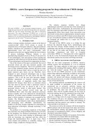
Growth ~10% p.a. 

I. INTRODUCTION 

A car is skidding and stabilizes itself without driver 

intervention; a laptop falls to the floor and protects the hard 

drive by parking the read/write drive head automatically 

before impact; an airbag fires before the driver involved in 

an impending automotive crash impacts the steering wheel 

thereby significantly reducing physical injury risk; – all 

these systems are based exclusively on MEMS sensors. 

These crucial MEMS sensor components of electronic 

control systems are making system reactions to human 

needs more intelligent, precise, and at much faster reaction 

rates than humanly possible. 

Important prerequisites for the success of sensors are their 

size, functionality, power consumption and costs. This 

technical progress in sensor development is realized by 

micro-machining. The development of these processes was 

the breakthrough to industrial mass-production for microelectro-mechanical 

systems (MEMS). Besides leading-edge 

micromechanical processes, innovative and robust ASIC 

designs, thorough simulations of the electrical and 

mechanical behaviour, a deep understanding of the 

interactions (mainly over temperature and lifetime) of the 

package and the mechanical structures are needed. This was 

achieved over the last 20 years by intense and successful 

development activities combined with the experience of 

volume production of billions of sensors. 

II. 

MARKET AND DRIVERS 

A. Market Size 

The growth of the MEMS market and the market 

segmentation is shown in Fig. 1 (source: iSuppli). Today’s 

market size is around 7 billion US dollars with four main 

segments: 

Source – iSuppli Corporation MEMS market tracker, H2 2010 

Figure 1: MEMS market 

• data processing (mainly ink jet printer nozzles) 

• automotive 

• mobile and consumer electronics 

• industry and process control 

B. Market Drivers for MEMS Sensors 

For MEMS Sensors there are several drivers which push 

new developments. In different markets the drivers are 

similar but have a different ranking. 

For automotive MEMS sensors the main drivers are: 

1. high functional requirements (high accuracy, selftest, 

advanced safety concepts) 

2. high reliability and quality (reliability for 15 years 

with failure rates of less than 1ppm under extreme 

environmental conditions) 

3. low price 

MEMS sensors for consumer electronics applications face 

different drivers: 

1. low price (

11-13 

May 2011, Aix-en-Provence, France 

 

Figure 2: Package roadmap of automotive acceleration sensors 

III. ACCELERATION SENSORS 

The success story of MEMS acceleration sensors started 

nearly 20 years ago with first high-g sensors for airbag 

applications and continued with low-g sensors for ABS, 

ESP, etc. Today over 90% of all new passenger cars are 

sold with an airbag system with at least one 

micromechanical acceleration sensor inside. These 

impressing equipment rates are only possible due to a 

continous and massive reduction of the costs of an airbag 

system and therefore also of the integrated acceleration 

sensor. This is achieved by strong improvements in the 

micromechanical sensing elements, the ASIC and – last but 

not least – the packaging. Fig. 2 shows the roadmap of 

packages for airbag acceleration sensors at Bosch. The first 

sensor, issued in the late 1970s, was a mechanical sensor 

element in a metal can. In the mid 1980s the first 

mechanical sensor followed with the ASIC integrated in the 

same metal package. It was supplanted in 1996 by the first 

generation of micromechanical acceleration sensors in a 

PLCC28 package. The current generation of airbag 

accelerometers, starting in 2010, uses a SOIC8 package. 

This corresponds to a size reduction of more than 85% in 14 

years. 

The massive size reduction was achieved by several steps 

in technology development. Due to design and process 

progress the micromechanical sensor element could be 

drastically reduced in size. The use of modern technologies 

in IC processes led to a steady decrease of the ASIC size at 

the same time – despite enhanced sensor performance and 

higher self-test capabilities. With sophisticated state of the 

art simulations – fed by the experience of several sensor 

generations and of far more than 1 billion sensors produced 

– key parameters of the package are optimized. The most 

important of those are 

• overall geometry (package height, length and width vs. 

die size, symmetry, …) 

• leadframe design (size, thickness, structure, …) 

• die-attach (material parameters like E-modulus, 

thickness,…) 

• mold compound (CTEs, …) 

• mold coverage (overall portion of mold compound vs. 

Silicon content of the package) 

The main hurdles for a more aggressive package size 

reduction are the the capability for further processing and 

the extreme environmental conditions automotive sensors 

have to withstand. 

Figure 3: Footprint of automotive and CE acceleration sensors 

Figure 4: Crosssection and SEM picture of BMA220 (© Chipworks) 

The consumer electronics (CE) industry has even higher 

constraints regarding package size (footprint as well as 

height). Bosch’s first acceleration sensor for CE in 2006 

reduced the automotive package size to a 4 4 mm² QFNpackage 

by half. Already one year later the size was further 

reduced to 3 3 mm². At the beginning of 2010 Bosch 

introduced the BMA220 - world’s first digital acceleration 

sensor in a 2 2 mm² LGA package. Fig. 3 shows the 

footprint development of automotive and CE sensors. 

One major step towards the 2 2 cm² package was the 

transition from side-by-side assembly to 3D stacked 

assembly. With this 3D Integration approach the ASIC is 

stacked on the micromechanical sensor element. Fig. 4 

depicts insights into the construction of the BMA220. 

IV. INERTIAL COMBI-SENSORS 

Sooner or later the further size reduction will become 

increasingly difficult. A new trend arises for sensors used in 

systems with a standard combinations of different sensors. 

An example are the inertial sensors used for vehicle 

dynamics control systems like ESP®. A typical ESP system 

needs the signals of a yaw rate sensor and an one or two 

axial low-g acceleration sensor. 

The first ESP systems were using a macro-mechanical 

yaw rate sensor, which was based on a piezoelectrically 

actuated, vibrating metal cylinder with piezo’s as sensing 

element of the Coriolis force [1], for detection of the car´s 

rotation along its vertical axis. In addition a mechanical 

single-axis low-g accelerometer has been applied to detect 

the vehicle´s dynamical state and for plausibilization of the 

yaw rate signal. 

2

11-13 


 

Figure 7: Package roadmap of yaw rate sensors for ESP 

specific readout circuit (ASIC) in a SOIC16w package (Fig. 

6). With this approach the footprint of the sensor could be 

reduced by 70% to the two predecessor sensors. 

Figure 5: SEM picture of Bosch’s first micromechanical yaw rate sensor 

(combination of bulk and surface micromachining) 

In 1998, as ESP systems were starting to gain broader 

market share, Bosch introduced its first silicon 

micromachined yaw rate sensor [2]. The sensing elements 

were manufactured using a mixed bulk and surface 

micromachining technology and have been packaged in a 

metal can housing (Fig. 5). 

Growing demand for new additional functions of ESP and 

of future vehicle dynamics systems – like Hill Hold Control 

(HHC), Roll Over Mitigation (ROM), Electronic Active 

Steering, and others – required the development of 

improved inertial sensors with higher precision at lower 

manufacturing costs. These goals have been achieved by the 

3 rd generation ESP sensors [3], a digital inertial sensor 

platform based on cost effective surface micromachining 

technology, which was released in 2005. 

Fig. 7 shows the development of the first mechanical yaw 

rate sensor to the current combined inertial sensor SMI540 

REFERENCES 

[1] A. Reppich, R. Willig, “Yaw Rate Sensor for Vehicle Dynamics 

Control Systems”, SAE Technical Paper 950537 (1995). 

[2] M. Lutz, W. Golderer. J. Gerstenmeier, J. Marek, B. Maihöfer, S. 

Mahler; H. Münzel, U. Bischof, in Proceedings of Transducers '97, 

Chicago, IL, June 1997, p. 847-850. 

[3] U. Gómez, B. Kuhlmann, J. Classen, W. Bauer, C. Lang, M. Veith, 

E. Esch, J. Frey, F. Grabmaier, K. Offterdinger, T. Raab, R. Willig, 

R. Neul, “New Surface Micromachined Angular Rate Sensor for 

Vehicle Stabilizing Systems in Automotive Applications”, in 

Proceedings of Transducers ’05, Seoul, June 2005, p. 184-187. 

Recent development at Bosch resulted in the world’s first 

integrated inertial sensor modules, combining different 

sensors (angular rate and low-g acceleration sensors) and 

various sensing axis (x, y) into one single standard mold 

package at low size and footprint (SMI540). In detail, the 

sensor consists of a combination of two surface 

micromachined MEMS sensing chips – one for angular rate, 

one for 2-axis acceleration – stacked onto an application 

Figure 6: Combined inertial sensor SMI540 for ESP 

3

11-13 


 

Dynamic Behavior of Resonant Piezoelectric 

Cantilevers Partially Immersed in Liquid 

M. Maroufi 1,2 ,Sh. Zihajehzadeh 1,3 , M. Shamshirsaz 1 , A.H. Rezaie 3 , M.B. Asgari 4 

1 New Technologies Research Center, 2 Mechanical Engineering Department, 3 Electrical Engineering Department 

Amirkabir University of Technology (Tehran Polytechnic), 4 Niroo Research Institute 

424 Hafez Ave., P.B. 15875-4413. Tehran, Iran 

E-mail: shamshir@aut.ac.ir 

Abstract 

Resonant Piezoelectric-excited Millimeter-sized Cantilevers 

(PEMC), has attracted many researchers' interest in the 

applications such as liquid level and density sensing. As in 

these applications, the PEMC are partially immersed in liquid, 

an appropriate analytical model is needed to predict the 

dynamic behavior of these devices. 

In this work, a PEMC has been fabricated for liquid level 

sensing. An analytical model based on Euler-Bernoulli theory 

and energy method is developed and applied to evaluate the 

performance of this device with respect to different tip 

immersion depth. To validate this model, the theoretical 

results are compared with the experimental results for the tip 

immersion depth from 0.5 mm to 9 mm in water. The 

simulation results are in almost good agreement with 

experimental data. The difference in natural frequency 

obtained by the theoretical model for different immersion 

depth remains less than 8%. The linear region of the natural 

frequency shift versus immersion depth has been identified to 

be from the depth of 9 to 11 mm. 


Nowadays, resonant Piezoelectric-excited Millimeter-sized 

Cantilevers (PEMC) have many applications as sensors. 

Among these diverse applications, are the ones where the 

cantilever is partially immersed in the liquid environment. In 

these cases, PEMC are used for online measuring of liquid 

density [1], [2], [3] or online determination of liquid level at 

micron resolution [4]. Online level detection of liquid is a 

powerful tool in many analytical processes where solvent 

concentration has to be monitored. 

Even though, there exists different tools for liquid level 

sensing such as ultrasonic, acoustic and optical methods, none 

of them is competent with PEMC, considering their ease of 

fabrication, small size and high performance [4].In fact, the 

performance of these devices for sensing application in liquid 

environment depends on many factors such as dimension of 

the cantilever and the piezoelectric layer, the immersion depth 

of the cantilever into liquid and so on. 

To evaluate the performance of PEMC partially immersed in 

liquid, a theoretical model is needed. Analytical model for the 

piezoelectric driven macro cantilever in air in introduced in [5] 

and also a model for the thermal driven cantilever wholly 

immersed in liquid with application in AFM is presented in 

[6]. 

In this work, a PEMC has been fabricated for liquid level 

sensing. The motivation is first to develop an analytical model 

to predict the dynamic behavior of PEMC partially immersed 

in liquid. This model is derived here based on Euler-Bernoulli 

theory and energy method. Further, this model could be 

utilized to investigate the effect of the different geometrical 

and material properties on the performance of these devices as 

future work. 

Second objective in this work is to identify the appropriate 

immersion depth range in which the resonant frequency 

changes due to immersion depth variation show a linear 

behavior in liquid level sensor application. 

To validate this model, the theoretical results are compared 

with the experimental results for the tip immersion depth from 

0.5 mm to 9 mm in water. The simulation results are in almost 

good agreement with experimental data. The difference in 

natural frequency obtained by the theoretical model for 

different immersion depth remains less than 8%. The linear 

region of the natural frequency shift versus immersion depth 

has been identified to be from the depth of 9 to 11 mm. 

II. THEORETICAL MODEL 

The fabricated PEMC is depicted schematically in Fig. 1. This 

structure consists of a millimeter sized steel beam as a 

cantilever on which a piezoelectric patch is attached. The 

cantilever is immersed partially in the fluid. Applying 

electrical AC voltage on the piezoelectric patch, the cantilever 

is forced to vibrate. 

To model the resonant cantilever partially immersed in liquid , 

three regions on the cantilever has been considered; a) first 

part where piezoelectric patch is bonded on the cantilever, b) 

middle part of cantilever where it vibrates freely ignoring air 

damping effect c) end part where the cantilever vibrates in the 

liquid. Also, three coordinate systems are assumed in each 

region (Fig. 1). 

4

11-13 


 

(3) 

In (3), d is the piezoelectric constant. To obtain E along 

piezoelectric thickness, it is assumed that an AC electrical 

voltage V is applied to piezoelectric patch. Using piezoelectric 

constitutive equation, the electrical field can be calculated by 

[5]: 

2 2 2 

 

2 

(4) 

Fig.1.Configuration of the PEMC partially immersed in liquid; three 

regions considered in theoretical model 

To achieve vibration equation of the cantilever accompany by 

piezoelectric patch the strain distribution along the thickness 

of the cantilever must be obtained. In Fig.2 the neutral axis 

position is demonstrated. In this figure the distance between 

neutral axis of the cantilever-piezoelectric from piezoelectric 

bottom layer is denoted by . It is assumed that the 

distribution of the strain along cantilever thickness is linear, so 

the strain at a distance x from the neutral axis is: 

 

 

(1) 

In which w is the transverse displacements of the cantilever. 

(w ) denotes twice derivation with respect to X 1 along the 

cantilever. 

In which t is the thickness of the piezoelectric. After 

Substitution (4) and (1) in (2), the energy of the piezoelectric 

layer can be obtained. To drive vibration equation, the 

Lagrangian for the piezoelectric layer and cantilever is 

calculated. So, the kinetic energy has to be solved. The mass 

per length for the first region of the piezoelectric cantilever in 

the kinetic energy calculation is defined as: 

(5) 

After calculation of the Lagrangian for both layers, the 

variation of the (6) is set to zero: 

 

 

0 (6) 

 

 

In which are the Lagrangian for each region. Using (6), the 

equation of motion and the boundary condition of the first 

region are determined. The equation of the motion is: 

2 2 0 (7) 

In (7), I , I are the moment of inertia of the piezoelectric 

patch and cantilever with respect to neutral axis respectively. 

A is the piezoelectric cross section area and Y is the Young 

modulus of the cantilever. a and a are defined as [5]: 

1 2 

 

(8) 

Fig.2:The position of the neutral axis with respect to piezoelectric patch 

and the coordinate X 3 along the cantilever thickness 

 

2 

8 

(9) 

To drive vibration equation of the first region of the cantilever, 

the energy stored in the piezoelectric can be determined by 

[5]: 

1 2 1 2 (2) 

Where Y is the Young modulus of the piezoelectric layer, E 

is the electrical filed along piezoelectric layer thickness due to 

applied voltage, is the dielectric constant. e is defined as: 

Using energy method also for the second region, the equation 

of the motion becomes [6]: 

0 (10) 

In the above equation, (w ) is the transverse displacement of 

the cantilever in the second region. To obtain solution in 

frequency domain, both (7) and (10) should be rewritten in 

frequency domain. (11) and (12) are the frequency domain 

expression of the (7) and(10) respectively: 

5

11-13 


 

, 2 2 

(11) 

, 0 

, TABLE 1 

, 0 (12) 

TABLE OF MATERIAL AND GEOMETRICAL PROPERTIES 

Property 

Cantilever 

Piezoelectric 

(Steel St304) (PZT5H4E) 

In the third region the vibration of the cantilever is affected by 

Young Modulus (GPa) 

the liquid presence. The force which is exerted by liquid to a 

193 62 

long vibrant cantilever in frequency domain is given in [7] Density (Kg/m 3 ) 8000 7800 

as: 

Length (mm) 36 6 

Width (mm) 3 3 

4 Γ , 

(13) 

Thickness(mm) 0.1 0.267 

Piezoelectric 

In (13), W is the transverse displacement of 

the cantilever in 

--- --- -320×10 

constant(m/V) 

-12 

the third region in frequency domain, ρ F is the density of fluid 

and b is the width of the cantilever. Γ is the hydrodynamic Relative Dielectric 

--- --- 3800 

function considering the viscosity and density of the displaced 

constant 

liquid [7]. Regarding the liquid force on the vibration of the 

cantilever, equation of the motion of the cantilever in 

The geometrical and material properties of the PEMC and 

frequency domain can be presented by: 

piezoelectric patch are given in TABLE 1. 

The natural frequency of the piezoelectric cantilever has been 

, , (14) determined by an impedance evaluation board, where the 

impedance phase angle attaints the maximum [4]. The 

To obtain the frequency response of the cantilever three experiments have been carried out to obtain natural 

equations developed above are solved simultaneously with frequencies of the PEMC for different immersion depth in 

appropriate boundary conditions. 

liquid. To vary this immersion depth, for each test, a known 

volume of water equivalent to 500μm liquid level change, is 

III. EXPERIMENTAL SETUP AND PROCEDURE 

added to container. 

The schematic of the experimental setup for liquid level 

sensing is shown in Fig. 3. The PEMC is mounted on a holder 

IV. RESULTS AND DISCUSSION 

which keeps PEMC at a fixed position in the 

liquid container 

during the experiments. 

The experimental and theoretical natural frequencies for each 

For the fabrication of the millimeter size cantilever, Electrical immersion depth in water are shown in Tab 2. As it can be 

Discharge Machining (EDM) is used to achieve the seen, the natural frequency decreases as the liquid level 

dimensional tolerances below millimeter. The piezoelectric increases. This decrease in natural frequency is due to a 

layer is cut by diamond knife and is attached to cantilever by greater displaced mass of liquid 

with the immersed cantilever 

cyanoacrylate adhesive. The schematic of the PEMC is shown part. 

in Fig. 4. 

The deviation percentage of theoretical results from 

experimental data defined as 

100 is also reported 

 

in this table. This deviation remains less than about 8% for 

different immersion depth. 

To examine the performance of 

the PEMC as a liquid level 

sensor, the curve of natural frequency shift versus immersion 

depth is presented in Fig. 5. In this figure, the middle region; 

from 9 to 11 mm immersion depths, not only the curve is 

linear but also it has the highest slope. 

Fig.3.Schematic of experimental setup for liquid level sensing 

Fig.4.Schematic of the PEMC 

TABLE 2 

COMPARISION OF THEORITICAL AND EXPERIMENTAL RESULTS IN WATER 

Immersion 

 

depth (mm) 

(Hz) 

6 4211 

7 4193 

8 4184 

9 4133 

10 4009 

11 3850 

12 3744 

13 3710 

14 3702 

(Hz) 

Deviation 

(%) 

4095.5 2.73 

4087 2.53 

4015 4.04 

3850 6.85 

3677.5 8.27 

3577 7.09 

3553 5.1 

3549 4.34 

3502 5.402 

6

11-13 


 

Fig.5.Experimental and theoretical natural frequency shift vs. immersion 

depth for water 

The sensor should be utilized in the region with the highest 

slope or highest sensitivity i.e. the highest frequency shift for 

each increment change in the immersion depth. 

It can be seen from Fig.5 that even though there is a slight 

difference between the theoretical and experimental curve, as 

the trend of the curves are similar, the dynamic behavior of the 

PEMC in liquid can be satisfactorily predicted by this 

theoretical model. The slight difference of theoretical results 

from the experimental data; a positive vertical shift 

accompanied with a negative horizontal shift, can be described 

as follow. First, theoretical model has been developed based 

on the assumptions for the simplicity of calculation such as the 

cantilever length and the container dimensions are assumed 

too long comparing with cantilever width and thickness, …[7]. 

Moreover, some of the mechanical and dimensional 

parameters have been ignored due to lack of measurement 

parameters. These parameters are the thickness of the adhesive 

layer and its mechanical properties, the effect of the clamp and 

the dissipation factor in piezoelectric and cantilever. Also, the 

values of the steel cantilever and the piezoelectric material 

properties such as the Young modules, density …are provided 

from literature, so there exists some uncertainties in 

parameters' values given in Tab. 1. Furthermore, in the 

experimental test there can be some errors in determining the 

exact volume of added fluid, and consequently in determining 

the immersion depth exactly. 

REFERENCES 

[1] Kishan Rijal, Raj Mutharasan, “Piezoelectric-excited millimetersized 

cantilever sensors detect density differences of a few 

micrograms/mL in liquid medium”, Sensors and Actuators B 124 

(2007) 237--244 

[2] Christian Riesch, Erwin K. Reichel,Franz Keplinger, and Bernhard 

Jakoby, “Characterizing Vibrating Cantilevers for Liquid Viscosity 

and Density Sensing”, Hindawi Publishing Corporation Journal of 

Sensors Volume 2008, Article ID 697062, 9 pages 

doi:10.1155/2008/697062 

[3] Wan Y. Shih,Xiaoping Li, Huiming Gu, Wei-Heng Shih and Ilhan 

A. Aksay,” Simultaneous liquid viscosity and density 

determination with piezoelectric unimorph cantilevers”, Journal of 

Applied Physics, Volume 89, Number 2, January 2001 

[4] Gossett A. Campbell, Raj Mutharasan,” Sensing of liquid level at 

micron resolution using self-excited millimeter-sized PZT 

cantilever”, Sensors and Actuators A 122 (2005) 326–334 

[5] Sudipta Basak, Arvind Raman, Suresh V. Garimella, “Dynamic 

Response Optimization of Piezoelectrically Excited Thin Resonant 

Beams”, Journal of Vibration and Acoustics FEBRUARY 2005 

Vol. 127 / 19 

[6] Singiresu .S. Rao, “ Vibration of continuous systems”, Wily 2007, 

PP. 321-338. 

[7] John Elie Sader, “Frequency response of cantilever beams 

immersed in viscous fluids with applications to the atomic force 

microscope”, Journal of Applied Physics, Volume 84, Number 1, 

July 1998 

[8] K. Fukuda, H. Irihama, T. Tsuji, K. Nakamoto, K. Yamanaka, 

Sharpening contact resonance spectra in UAFM using Q-control, 

Surf. Sci. 532, 535 (2003) 1145–1151. 

V. CONCLUSION 

A PEMC with a test set-up have been fabricated for liquid 

level sensing. An analytical model to predict the dynamic 

behavior of partially immersed PEMC in liquid environment is 

developed. The validity of the model is examined by 

comparison of simulation results with the experimental data 

for different immersion depth of the PEMC in water. The 

difference in natural frequency obtained by the theoretical 

model for different immersion depth remains less than 8%. A 

linear region for sensing related to immersion depth from 9 to 

11 mm is identified where the sensitivity is maximum. 

7

11-13 


 

Reliable system-level models for electrostatically actuated 

devices under varying ambient conditions: 

Modeling and validation 

Gabriele Schrag, Martin Niessner, Gerhard Wachutka 

Institute for Physics of Electrotechnology, Munich University of Technology 

Arcisstr. 21, D-80290 München, Germany 

email: schrag@tep.ei.tum.de 

Abstract- We present a physics-based multi-energy domain 

macromodel that allows – in general – for the efficient simulation 

of any electrostatic actuator within standard IC frameworks and 

apply it exemplarily to an RF-MEMS switch. The predictive 

power of this macromodel, which depends crucially on the 

quality of the applied damping and contact models, has been 

evaluated by white light interferometer and laser vibrometer 

measurements. It turned out that the models for viscous damping 

as well as for the electromechanical energy domain are in very 

good agreement with the experiments while the applied standard 

contact model fails in reproducing the measured contact 

phenomena. Based on these findings suggestions for improved 

system-level contact models are discussed. 

investigation of the performance of the models for varying 

pressure conditions and during the phase of initial contact, 

since these phenomena have decisive impact on the closing 

behavior of the considered switch and all MEMS actuators 

operating in contact mode. 

I. MOTIVATION AND PROBLEM DESCRIPTION 

A key prerequisite for the routine use of 

microelectromechanical actuators like radio frequency (RF- 

MEMS) switches, e.g., as standard circuit elements is the 

availability of computationally efficient, but yet physics-based 

and, thus, predictive models, which correctly describe their 

operation. Furthermore, these models should be compatible 

with a framework that allows for an integrated design of 

semiconductor-based circuits with MEMS hybridization. The 

simulation of the switching behavior, i.e. of the pull-in and 

pull-out transients of such devices, is, however, a challenging 

task because multiple energy domains and their nonlinear 

interactions have to be taken into account, i.e. the electrostatic 

actuation of the mechanically moving parts, viscous air 

damping and contact forces during impact. The preferred 

method for enabling the fast simulation of such pull-in/-out 

transients is therefore not the use of complex and 

computationally expensive finite element models but of multienergy 

domain coupled macromodels with a highly reduced 

number of degrees of freedom that are by far more efficient and 

can be simulated within standard integrated circuit (IC) design 

frameworks. 

In the following, we present physics-based macromodels 

suited, in general, for the design of electrostatically actuated 

and viscously damped actuators which operate under dynamic 

pull-in conditions and apply it to an RF-MEMS switch. The 

derived models, which can be directly used for co-simulation 

with electronic circuits in standard IC design frameworks, are 

evaluated w.r.t. measurements carried out with a white light 

interferometer (WLI) and a laser Doppler vibrometer (LV), 

respectively. Special emphasis has been placed on the 

Figure 1. Measured (WLI) 3D profile of the RF switch without bias. 

Figure 2. Measured (WLI) profile of the electrodes and the 12 elevated 

contact pads. The membrane was removed for this measurement. 

II. 

contact 

pads 

DEMONSTRATOR AND EXPERIMENTAL SETUP 

A 3D white light interferometer profile of the considered 

RF-MEMS switch is depicted in fig. 1. The switch has been 

fabricated at Fondazione Bruno Kessler (FBK) in Trento [1] 

and consists of a movable perforated gold membrane 

suspended above a fixed ground electrode through four straight 

beams. The fixed ground electrode acts as actuation electrode 

of the switch and consists of several lateral fingers that are 

connected in parallel (cp. fig. 2). By applying a voltage, the 

8

suspended membrane can be pulled towards the ground 

electrode, collapses onto 12 elevated contact pads and closes an 

ohmic contact so that the RF signal path is closed. 

The topography of the switches has been analyzed by applying 

a white light interferometer (Veeco NT1100 DMEMS) and the 

dynamics has been characterized by recording the transient 

deflection of the moving membrane by a single spot laser 

Doppler vibrometer (Polytec OFV-5000). An on-purpose 

developed vacuum chamber with pressure control enables the 

characterization of the microstructures under varying pressure 

conditions in order to evaluate the applied models for viscous 

damping. The experimental set up is shown in fig. 3. 

11-13 


 

using the single point laser Doppler vibrometer depicted in 

fig. 3, parameters like the pull-in/pull-out voltages (and from 

that the actual gap height) or the resonance frequency of the 

mechanical structure could be extracted. The parameters of the 

investigated switch, which are the basis of our models, are 

summarized in detail in table 1 below. 

Table 1. Technical data of the investigated RF-MEMS switches. For the 

electrode and the substrate, the gap width is given between the membrane and 

the dielectric layers. 

Membrane 

Suspensions 

Thickness 5.2 µm Thickness 2.0 µm 

Length 260 µm Length 165 µm 

Width 140 µm Width 10 µm 

A 

Side length of 

holes 

Spacing between 

holes 

20 µm 

20 µm Other 

Resonance frequency 

14.7 kHz 

C 

B 

C 

Gap widths 

Membrane to 

contact pad 

Membrane to 

electrode 

Membrane to 

substrate 

Thickness of 700 nm 

dielectric on 

electrode 

1.7 µm Pull-in voltage 29-30 V 

2.7 µm Release voltage 22-26 V 

3.4 µm Effective residual 

air gap (g min ) 

~20-50 nm 

Figure 3. Photograph of the laser vibrometer (A) and the on-purpose 

developed pressure chamber (B). Two pressure sensors (C) are used to 

control the pressure inside the chamber . 

Displacement [μm] 

0.4 

0.2 

0 

-0.2 

-0.4 

-0.6 

-0.8 

-1 

-1.2 

-1.4 

-1.6 

-1.8 

-30 -20 -10 0 10 20 30 

Voltage [V] 

Figure 4. Quais-static pull-in/pull-out characteristic of the RF MEMS 

switch. A trinangular waveform with zero mean voltage and 70 V amplitude 

(peak to peak) at a frequency of 1 Hz has been applied. The pull-in voltage 

lies between 29 V and 30 V, the release voltage between 23 V and 26 V. 

As a first guess, the parameters of the switch have been taken 

from the technical data given by the process description and 

the design. In order to include also the manufacturing 

tolerances in our model and, thus, to enhance its accuracy, 

optical measurements appling a white ligth interferometer (see 

fig. 1 and 2) have been carried out in order to extract the exact 

dimensions of the device (electrode, contact pads, membrane 

thickness, e.g.). From the quasi-statically measured pull-in and 

pull-out characteristics (see fig. 4) and dynamic measurements 

III. MODELING AND THEORETICAL BACKGROUND 

The macromodel of the switch is derived on the basis of the 

hierarchical modeling approach as reported in [2], which is 

strictly based on flux-conserving reduced-order and/or compact 

modeling techniques, so that the resulting system-level models 

are rigorously formulated in terms of conjugated variables 

(”across”- and ”through”-variables) and the generalized 

Kirchhoffian network theory can be used as a theoretical 

framework for the formulation of the entire system model. 

Starting point of the modeling procedure is the decomposition 

of the device into tractable subsystems. In this particular case, 

these are the mechanical subsystem represented by the 

perforated membrane and the four flat suspension springs, the 

electrostatic subsystem, accounting for the electric field 

between the perforated membrane and the actuation electrode 

(see Fig. 2), and the fluidic subsystem comprising the ambient 

air that exerts damping forces on the moving parts of the 

structure. Additionally, adequate compact models have to be 

derived that describe the closing phase of the switch properly. 

The basis for the mechanical submodel of the suspended 

membrane is the modal superposition technique described in 

[3]. The eigenmode shapes and frequencies of the suspended 

membrane are calculated in a FEM simulation tool. The most 

significant modes – in the case of the considered switch the 

fundamental and the next higher completely symmetric 

eigenmode – are identified and used to formulate a 

macromodel in terms of modal amplitudes consisting of only 

one second-order differential equation per included eigenmode. 

9

11-13 


Residual stress in the suspended membrane induced by the 

 

Here, q denotes the vector of modal amplitudes, φ 

pad , n 

the 

fabrication process has been taken into account by calibrating 

the fundamental eigenfrequency to the measured one. 

averaged modal shape factor for the n-th contact pad, 

The submodel for the electrostatic forces exerted by the 

ground electrode is derived in two steps. First, the electrostatic 

energy, which is stored between a single electrode finger and 

the membrane, is determined in terms of the modal amplitudes. 

Second, Lagrangian energy functionals are calculated for each 

eigenmode and are included as electrostatic actuation term in 

the respective eigenmode equation of the mechanical model. 

In order to take into account the viscous damping forces the 

mixed-level approach as presented in [4] is applied. It is based 

on the Reynolds equation, which is evaluated by applying a 

fluidic Kirchhoffian network distributed over the device 

geometry. At perforations and outer boundaries lumped 

physics-based fluidic resistances are added accounting for the 

additional pressure drops at these locations (see fig. 5). 

Consequently, this mixed-level model does not constitute a 

pure lumped element model and – depending on the granularity 

of the finite network – still exhibits a rather larger number of 

degrees of freedom. However, the advantage of this approach is 

that it can be tailored to the topography of the real structure, i.e. 

take into account all perforations and – in the case of the 

considered switch – also locally varying gap heights which 

occur due to the elevated contact pads and electrode fingers. 

ambient pressure 

P 0 

moving 

plate 

{ 

finite network 

R O 

R C 

R T 

fixed plate 

moving 

plate 

{ 

finite network 

Figure 5. Illustration of the mixed-level model. Models for holes are 

embedded in the finite network solving the Reynolds equation. The resistor R T 

models the region, where the fluid enters the channel. The resistor R C models 

the channel resistance; R O models the orifice flow [5,6]. 

The mechanical contact that occurs, when the switch is 

closed, is included into the mixed-level model by adding 

contact forces at the respective locations above the contact 

pads. The modal formulation of these forces reads as follows: 

12 

⎧ 

⎪ 

( ) 

∑ φpad , n 

⋅kcontact , n 

⋅gn ( q) if gn 

( q) 

≤0 

Fcontact, total, 

i 

q = ⎨ (1) 

n= 

1 

⎪⎩ 0 else 

k 

contact, 

n 

the lumped contact stiffness of the n-th pad and gn 

( ) 

q the 

locally averaged displacement at the n-th pad. 

This model enables to simulate also bouncing during the 

landing phase of the membrane. In order to avoid numerically 

undesired discontinuities resulting from the if-then-else 

construct proposed in previous work [7], we now use a 

function Θ 

n 

based on the tanh-function instead, in order to 

implement a more stable transition into the contact state: 

⎛ ⎛ gn 

Θ 

n ( q) 

= 0.5⋅⎜1−tanh 

⎜ 

⎜ ⎜ β 

⎝ ⎝ 

( q) 

⎞⎞ 

⎟⎟ 

⎟⎟ 

⎠⎠ 

β denotes a parameter controlling the smoothness of this 

transition. The complete contact formulation then reads: 

12 

( ) = Θ ( ) ⋅φ 

⋅ ⋅ ( ) 

F q ∑ q k g q (3) 

contact , total , i n pad , n contact , n n 

n= 

1 

The compact model of the entire switch is then assembled 

by formulating all submodels in terms of the modal amplitudes 

and combining them with the mechanical submodel: 

2 7 

2 Vb 

∂Ck( q) 

T 

i 

+ ωi i 

= ∑ + θi 2 k = 1 ∂qi 

 

ext, i 

 

0 

F el 

q 

q F ( qq , , p) 

Here, q i and ω i denote the amplitude and the frequency of 

the i-th eigenmode, θ i 

denotes the vector of the respective 

discretized mode shape, Ck 

( q ) stands for the capacitance of 

the k-th electrode finger and V k for the respective applied 

voltage. F ext represents the vector of external forces comprising 

in this case the models for damping and contact forces. 

Finally, the derived macromodels of the subsystems are 

formulated in terms of conjugated variables (”across”- and 

”through”-variables) and interlinked to form a generalized 

Kirchhoffian network, which inherently governs the exchange 

of energy and other physical quantities through Kirchhoff’s 

laws and can be implemented easily in any standard system 

simulator of an IC framework (in this work: Spectre from the 

Cadence IC design suite). 

IV. EXPERIMENTAL VALIDATION OF SIMULATED RESULTS 

The macromodel was evaluated w.r.t. measurements 

performed with a laser Doppler vibrometer (LV) and a white 

light interferometer (WLI). A pressure chamber as depicted in 

fig. 3 was used to enable measurements at different pressure 

levels. 

First, the combined electro-mechanical model was validated 

against the quasi-statically measured pull-in/pull-out 

characteristic of the membrane (see Fig. 6). It shows good 

agreement with the pull-in characteristic, but yields an 

incorrect pull-out voltage. Since the electromechanical model 

works quite accurately for the pull-in curve, this discrepancy is 

(2) 

(4) 

10

most likely due to not yet considered adhesion forces and other 

contact-related phenomena. 


0.4 

0.2 

0 

-0.2 

-0.4 

-0.6 

-0.8 

-1 

-1.2 

Measurement 

-1.4 

MLM 

-1.6 

-1.8 

0 5 10 15 20 25 30 

Voltage [V] 

Figure 6. Measured and simulated quasi-static pull-in/-out characteristics of 

the membrane. The curves have been taken using the laser vibrometer and 

actuating the membrane electrostatically with a voltage of 70 V (peak to peak) 

of triangular wave form at a frequency of 1 Hz. 

Second, we evaluated the transients of the device at an 

ambient pressure ranging from 960 mbar to 1 mbar. Figure 7 

shows the measured and simulated response of the switch to a 

square wave voltage of 25 V, a voltage which is lower than the 

pull-in voltage. The membrane responds in the first half of the 

period (0..2.5ms) with a damped oscillation at a mean 

displacement of about 420nm. After voltage has been turned 

off (t > 2.5ms), it releases to its original position undergoing 

damped oscillations. 

0.4 

0.2 

Measurement 

MLM 

11-13 


 

Additionally, we evaluated the limits of the fluidic damping 

model by extracting the quality factor Q as a measure for 

viscous damping from the transients recorded for varying 

ambient pressure values. Since for pressures lower than 

100 mbar the Q-factor is limited by another mechanism than 

squeeze film damping, we extracted the value Q LIMIT for this 

damping mechanism from experiments and added it to the Q- 

factor Q SQFD calculated from our mixed-level damping model 

according to 

Q TOTAL -1 = Q LIMIT 

-1 

+ Q SQFD 

-1 

Fig. 8 reveals that our model is in very good agreement – 

within an error of about 7% to 10% – to the measured data for 

moderately high pressure values from normal pressure down to 

about 100 mbar. Below pressures of about 100 mbar a 15% 

error limit between simulated and measured Q-values is 

exceeded. This is certainly due to the large variance of the 

correction factors accounting for gas rarefaction effects, which 

can be found in literature. Systematic investigations on 

dedicated test structures are focus of on-going work in order to 

get a better data base for the physical understanding of gas 

damping in this regime [9]. 

Quality factor 

Q MLM 

Q MEAS 

(5) 

10 2 Pressure [mbar] 


0 

-0.2 

-0.4 

-0.6 

-0.8 

0 1 2 3 4 5 

Time [ms] 

Figure 7. Measured and simulated response of the membrane. 

Actuation: rectangular voltage waveform (200 Hz; amplitudes 25 

V (on) and 0 V (off)). Ambient pressure: 960 mbar. 

The very good agreement of simulation and measurement 

in the second half of the time period (2.5..5ms) proves the 

accuracy of the damping model, while the good agreement in 

the first half of the period proves that the model correctly 

reproduces the electrostatic spring softening, which essentially 

decreases the resonance frequency of the switch during 

actuation, and the increased damping due to the decreasing gap 

height. Models of switches without physically-based 

description of gas damping fail at this point [8]. 

10 1 10 0 10 1 10 2 10 3 

Figure 8. Simulated and measured Q values calculated from the frequency 

spectrum using the half power method (“3dB bandwidth”). Remark: The 

measured sample exhibited an increased gap (plus about 300 nm ). 

In order to check the contact model, we actuated the 

device with a step voltage of 35 V, a voltage higher than the 

pull-in voltage (see fig. 9), in order to force the structure into 

contact and, subsequently, to release it again. 


1.4 

1 

0.6 

0.2 

-0.2 

-0.6 

-1 

-1.4 

Measurement 

MLM 

-1.8 

0 1 2 3 4 5 

Time [ms] 

Figure 9. Response of the membrane to a rectangular waveform (200Hz): 

amplitudes 35V (on) and 0V (off). Pull-in/contact occurs. 

11

A detailed analysis of the frequency spectrum of the 

landing phase (fig. 10) as well as of the release phase (with and 

without contact, i.e. actuation voltages of 35 V and 25 V, 

respectively, fig. 11) reveal that these phases are dominated by 

an intricate interplay of different mechanical vibrations. 

Peak-normalized 

amplidute (dB) 

Peak-normalized 

amplitude (db) 

0 

-10 

-20 

-30 

-40 

-50 

87 kHz 218 kHz 

-60 

0 50 100 150 200 250 300 

Frequency (kHz) 

Figure 10. Frequency spectrum of the measured landing phase of the 

membrane. Applied voltage 35V, frequency 250Hz. 

0 

-10 

-20 

-30 

-40 

-50 

14.7 kHz 

136 kHz 

35V (after pull-in) 

25V (no pull-in) 

-60 

0 50 100 150 200 250 300 


Figure 11. Frequency spectrum of the measured release phase of the 

membrane. Applied voltage 35V and 25V, resp.; frequency 250Hz. 

The modes at 14.7 kHz and 136 kHz occurring during 

release after the membrane was in contact with the contact pads 

(see black curve in fig. 11) correspond to the natural 

eigenfrequencies of the membrane. The notable contribution of 

the mode at 136 kHz compared to the spectrum where no pullin 

occurred (blue curve in fig. 11) leads us to the assumption 

that kinetic energy of the fundamental mode is transferred to 

the next higher symmetric mode during impact. Analyzing the 

landing phase of the switch by FFT (fig. 10) gives evidence of 

several superimposed vibrations at higher frequencies (see two 

modes at 87 and 218 kHz), which are obviously involved in 

the contact process. The high frequencies are supposed to be 

due to the high contact stiffness which now couples with the 

stiffness of the suspended membrane. Thus, the contact 

physics can only be captured correctly, when multiple and also 

higher modes and the coupling between them are implemented 

in the macromodel. Fig. 12 (top) shows a zoom of the closing 

transient displayed in fig. 9, where only the first 100μs are 

shown. It can be observed that our simulation model captures 

the landing phase already remarkably well, while models of 

Iannacci [10] and the commercial simulation tool Architect3D 

[11] that have been applied for benchmarking cannot 

reproduce the landing phase as well and, in particular, the 

Architect3D model overestimates the closing time 

considerably (see fig. 12, bottom). We assume that the good 

11-13 


 

agreement of our model is due to the fact that the mechanical 

part of our model, by its nature, already includes different (and 

also higher) mechanical eigenmodes. 



0 

-0.2 

-0.4 

-0.6 

-0.8 

-1 

-1.2 

-1.4 

-1.6 

Measurement 

MLM 

-1.8 

0 10 20 30 40 50 60 

Time [μs] 

0 

-0.2 

-0.4 

-0.6 

-0.8 

-1 

-1.2 

-1.4 

-1.6 

Measurement 

Architect3D 

Iannacci 

-1.8 

0 20 40 60 80 100 

Time [μs] 

Figure 12. Top: Zoom of the closing transient of fig. 9. Only the first 60μs are 

shown. The measurement is compared with simulated data from the MLM 

model. Bottom: Zoom of the closing transient of fig. 9. Only the first 100μs 

are shown and compared to two alternative macromodels (Iannacci[10] and 

Architect3D[11]), which have been applied for benachmarking. 

V. CONCLUSIONS 

We presented a physics-based multi-energy domain 

macromodel for an electrostatically actuated RF MEMS switch 

working under ambient pressure. It shows very good agreement 

with the measured quasi-static pull-in characteristic, with the 

non-contact transient measurements for ambient pressures 

down to 100 mbar and the pull-out transient after contact. 

However, the macromodel fails in reproducing the quasi-static 

pull-out characteristic and the contact phase properly. A FFT of 

the measured transients revealed that during impact of the 

membrane multiple structural modes are involved so that this 

phase can only be captured correctly by taking them and their 

interactions properly into account. Obviously, standard contact 

models are not yet accurate enough to reproduce this phase 

correctly. However, it showed that a mechanical model based 

on modal superposition techniques, i.e. a model where, by its 

nature, several eigenmodes are included, reproduces the 

landing phase best compared to other standard models. A 

sensitivity analysis showed that, together with the proper 

12

11-13 


description of the contact phase, accurate, physics-based 

 

damping models are a prerequisite for reliable and predictive 

modeling of MEMS actuators. An on-going comparative study 

given in [9] demonstrates this impressively. Future research 

will therefore focus on the physics during the impact of the 

membrane and how it can be captured in a system-level 

macromodel. Additionally, systematic experimental and 

theoretical investigations on viscous damping in the rarefied 

gas regime have to be carried out in order to gain a better data 

base and, thus, a better understanding of the underlying physics 

in order to include this effect correctly in our models. 

[1] J. Iannacci, F. Giacomozzi, S. Colpo, B. Margesin and M. Bartek, 

“A General Purpose Reconfigurable MEMS-Based Attenuator for 

Radio Frequency and Microwave Applications”, in Conf. Proc. of 

EUROCON, 2009, pp: 1201-1209 

[2] G. Schrag, R. Khaliliyulin, M. Niessner, and G. Wachutka, 

“Hierarchical Modeling Approach for Full-System Design and 

control of Microelectromechanical Systems,” in Conf. Proc. of 

Eurosensors XXII, 2008, pp. 528-531. 

[3] L. Gabbay, J. Mehner, and S. Senturia, “Computer-aided 

generation of reducedorder dynamic macromodels - I: 

Geometrically linear motion,” J. Microelectromechanical Systems, 

vol. 9, 2000, pp. 262–269. 

[4] Schrag G., and Wachutka G., “Physically based modeling of 

squeeze film damping by mixed-level system simulation,” Sensors 

and Actuators A, vol. 97-98; 2002 , pp. 193–200. 

[5] R. Sattler, “Physikalisch basierte Mixed-Level Modellierung von 

gedämpften elektromechanischen Systemen“, Shaker Verlag, 

Aachen, 2007. 

[6] M. Niessner, et al., “Experimentally validated and automatically 

generated multi-energy domain coupled model of a RF-MEMS 

switch”, Proc. EuroSimE 2009, Delft, NL, April 27-29, 2009, pp. 

595-600. 

[7] M. Niessner, G. Schrag, G. Wachtuka and J. Iannacci, “Modeling 

and fast simulation of RF-MEMS switches within standard IC 

design framework,” Proc. SISPAD 2010, Bologna, Italy, 

September 6-8, 317-320 (2010). 

[8] L. del Tin, et al., Digest Tech. Papers of 14 th Int. Conf. on Solidstate 

Sensors, Actuators and Microsystems (Transducers’07), 

Lyon, June 10-14, pp.635-638, 2007.. 

[9] M. Niessner, G. Schrag, J. Iannacci, G. Wachutka, “Mixed-level 

modeling of squeeze film damping in MEMS: Simulation and 

pressure-dependent experimental validation, accepted for 

publication at 16 th Int. Conf. on Solid-state Sensors, Actuators and 

Microsystems (Transducers’11), Beijing, China, June 5-9, 2011. 

[10] J. Iannacci, R. Gaddi and A. Gnudi,, “Experimental Validation of 

Mixed Electromechanical and Electromagnetic Modeling of RF- 

MEMS Devices Within a Standard IC Simulation Environment,” 

Journal of Microelectromechanical Systems 19 (3), 526-537 

(2010). 

[11] Coventor, Inc. [Coventorware Architect Version 2008.10 

Reference] (2008). 

13

11-13 


 

Investigation on the effect of geometrical dimensions 

on the conductive behaviour of a MEMS convective 

accelerometer 

A.A. Rekik 1,2 , B. Mezghani 2 , F. Azaïs 1 , N. Dumas 1 , M. Masmoudi 2 , F. Mailly 1 , P. Nouet 1 

1 LIRMM - CNRS/Univ. Montpellier 2 - 161 rue Ada, 34095 Montpellier, France 

2 ENIS - University of Sfax - Route Soukra, BP 1173 3038 Sfax, Tunisia 

Abstract— This paper presents an investigation on the effect 

of geometrical dimensions on the conductive behaviour of a 

CMOS MEMS convective accelerometer. Numerous FEM 

simulations are conducted to prove the validity of a previously 

developed model. This model was firstly developed to 

represent the effect of only one geometrical parameter; the 

etched cavity depth. We prove here that this model may 

represent also the effect of other geometrical parameters, the 

cavity half-width and the package height, on the conductive 

behaviour of the sensor. 

Keywords— MEMS, convective accelerometer, heat 

conduction, modelling. 


CMOS MEMS convective accelerometer is one example 

of a monolithically integrated sensor system. Such 

accelerometers present several advantages compared to the 

commonly used capacitive ones [1-2]. In addition to low 

cost batch fabrication, convective accelerometers are able to 

survive and sense very high shocks [3]. Mechanical rigidity 

and low mass are the main reasons that insure robustness to 

large accelerations. Unfortunately, and as it is generally the 

case for monolithic structures, strict requirements for 

process compatibility usually limit the performance level 

and potential applications [4-5]. To take advantage of the 

benefit of such a sensor, one use a system level design 

approach that requires an accurate and complete model of 

the sensor. This is considered as a vital and important step 

to help in predicting and/or increasing the overall system 

performance. One possible strategy is then to optimize the 

sensor dimensions to cope with the specifications and to 

adapt the global architecture accordingly. 

Existing models allow understanding the behaviour of a 

given sensor or studying geometry variations in a single 

dimension [6]. For multiple parameter variations, evaluation 

of geometrical and material properties in convective 

accelerometers is only possible through Finite Element 

Modelling (FEM) [7-8], which is very time consuming and 

meaningless. At the contrary, compact models allow a quick 

exploration of broad design spaces and a physical 

understanding of parameter influences. In a previous work 

[9], we have proposed a sensor model in which physicallybased 

expressions were developed to describe the 

conductive behaviour of a thermal accelerometer. This 

preliminary model was only including the effect of a single 

geometrical parameter (the depth of the bottom cavity, h 1 in 

Fig.1) since this parameter is the most difficult to control; it 

depends on the concentration of the etching solution and on 

the etching time. Initially developed to validate test 

methods, this model was then considered to validate system 

level architectures. Additional geometrical parameters 

appeared to be critical parameters for the design of the 

sensor. Therefore, the impact of these parameters has been 

investigated and a fully parameterized model is today 

introduced in this paper. 

In section 2, we briefly describe the accelerometer. In 

section 3, we present the previously published model of the 

sensor and we focus on the conduction part (heater source 

and common mode). Using FEM simulations, the effect of 

sensor dimensions on the conductive behaviour of the 

device is investigated in section 4. Finally, the proposed 

model validity is demonstrated over a large range of 

geometrical dimensions. 

II. ACCELEROMETER PRESENTATION 

The device under study is a convective accelerometer 

obtained by Front-Side Bulk Micromachining (FSBM) of a 

CMOS die fabricated in a 0.8 µm technology from Austria 

Microsystems® (Fig.1). Main lateral dimensions are the 

half-width of both the heater beam (r 1 ) and the cavity (r 2 ), 

and the distance between the heater and one detector (d). 

The three thin bridges are composed of the CMOS process 

back-end layers (oxide, polysilicon, aluminium, and 

nitride). In particular, polysilicon is used to implement 

resistors, for both heating (R H ) and temperature sensing 

(R D1 , R D2 ). The heater R H is powered by an electrical voltage 

(U H ) to create a temperature gradient in the bottom (i.e. 

etched silicon) and top (i.e. package) cavities: the 

temperature is then maximum at the heater location and 

minimum at the cavity boundaries. 

In absence of acceleration, the temperature detectors (R D1 , 

R D2 ) are located on an identical isotherm for symmetry 

reasons. Under acceleration along the AA’-axis, the free 

convection deforms the cavity temperature distribution so 

14

that detectors may measure the differential temperature. 

Indeed, polysilicon resistivity exhibits high temperature 

dependence (Temperature Coefficient of Resistance, 

TCR=9×10 -4 /°C) and the thermal signal is easily converted 

into a voltage by means of a Wheatstone bridge. This 

voltage is then amplified by an instrumentation amplifier. 

For more details on sensor manufacturing and 

characterization, please refer to previous works from some 

of the authors [8-11]. 

Heater 

Detectors 

11-13 


 

The model is composed of four main blocks (Fig.2). First, 

the heater temperature (T H ) is calculated from the external 

power supply (U H ). Then, the common mode temperature is 

calculated from the heater temperature. The heater 

temperature (T H ) and the common mode temperature (T CM ) 

are governed by the heat conduction in the fluid. Regarding 

fluid convection, the differential temperature (ΔT D ), resulting 

from acceleration, is calculated with an empirical expression 

that involves fitting parameters. Finally, regarding 

transduction, both detector resistances (R Di ) are deduced 

from their TCR factor. 

In this paper, we will focus on the conduction part only 

(heater and common mode). 

Amplifier A1 

Sensing 

direction 

(AA) 

A. Heater source 

During normal operation, the heating bridge is powered by 

a DC voltage (U H ) in order to set an initial temperature 

distribution in the cavity. The average heater temperature 

(T H ) is directly linked to the electrical power (P H ) with a 

linear relationship: 

Figure 1. SEM picture of the prototype and geometrical parameters: 

r 1=20μm, r 2=350μm, d= 125μm, h 1=300μm, h 2=1000μm. 

III. ACCELEROMETER MODEL 

For defect simulations, a previously developed high level 

model [11] has been improved to include the effect of 

etching defects [9]. This model only takes into account the 

effect of the bottom cavity depth h 1 . No other sensor 

dimensions were included. In addition, this model was 

developed for fixed values of cavity half-width (r 2 =350µm) 

and package height (h 2 =10mm). 

T 

T 

Rth 

P 

T 

Rth 

2 

UH 

HAHHA 

⋅+=⋅+ 

(1) 

RH 

where T A is the ambient temperature, R H is the electrical 

resistance of the beam and Rth H is the thermal resistance of 

the heater beam. 

The temperature dependence of the electrical resistance is 

taken into account in the power dissipation with: 

R 

R 

( 1 TCR T ) 

Δ ⋅+= 

(2) 

0 HH 

where TCR is the temperature coefficient given by the 

foundry and R H0 is the nominal value of the heater resistance 

at a reference temperature T 0 . This electrical resistance is 

obviously independent of the cavity depth but only depends 

on the heating resistance size and material properties. 

In contrast, the thermal resistance of the beam depends not 

only on the beam dimension but also on its geometrical 

environment: 

Rth 

H 

= 

1 

⋅ Sh 

where S=54.7×10 3 µm² denotes the exchange surface 

between the beam and the fluid given by 2(2r 1 +e)L, with L 

the beam length and e the beam thickness. 

The heat transfer coefficient h H depends on the heater 

temperature, the ambient temperature, the geometry of the 

heater beam and the geometry of its environment. 

Assuming a cylindrical heater with a radius R 1 at a 

temperature T H surrounded by a cylindrical cavity with a 

radius R 2 at a temperature T A , the heat transfer coefficient h H 

is given by [9]: 

H 

(3) 

Figure 2. Block diagram of the sensor model. 

h 

H 

= 

1 

(4) 

⎛ 

2 2 

3 3 

4 4 

λ 

⎞ 

0 ⎜ 

δ H1 −TT 

A δ H2 −TT 

A δ3 

H −TT 

A 

1+⋅ 

+ ⋅ + ⋅ ⎟ 

⎛ R ⎞ 

⎝ 

2 − AH 3TT 

− AH 4TT 

− 

AH 

⋅ 

⎠ 

⎜ 

2 

l ⎟ nR 

⎝ R1 

⎠ 

15

11-13 


 

where λ 0 =-3.9333×10 -4 Wm -1 K -1 is the air conductivity 

extrapolated at 0K. The three parameters δ 1 =-0.2589 Wm -1 K - 

2 , δ 2 =1.2349×10 -4 Wm -1 K -3 and δ 3 =-3.8662×10 -8 Wm -1 K -4 

represent the coefficients of thermal conductivity variation 

for the air. We have shown in [9] that, for the complex 

geometry of our accelerometer, expression 4 is still valid if: 

• R 1 is a trade-off between the radius of a cylinder with 

a perimeter equivalent to the heater bridge and the radius of 

a cylinder that contains the heater beam. 

• R 2 is a function of the bottom cavity depth h 1 : 

h 

rR ⋅= 

(5) 

1 

22 

4 

4 ⎛ r 

4 

2 ⎞ 

h1 

+ ⎜ 

⎝ 2 ⎟ ⎠ 

where the polynomial degree and the root order were 

chosen to obtain the best fit in two regions : a linear one 

obtained for low values of h 1 and a saturation region at r 2 

obtained for high values of h 1 . This model was developed for 

fixed values of r 2 and h 2 (350µm and 10mm, respectively). 

Also, it is found that the transition distance between the two 

regions seemed to be equal to r 2 /2. However, a parametric 

study on r 2 and h 2 should be conducted to confirm that it was 

not only a coincidence. 

B. Common mode 

Considering the same cylindrical geometry assumption, 

the relationship between the common mode temperature 

T CM , at a distance d from the center (R 1

2) Cavity width effect 

To verify the influence of the cavity half-width r 2 on the 

conductive behaviour of the sensor, a FEM simulation is 

performed for a new set of parameters: r 2 =700µm, 

h 1 =600µm, h 2 =10mm and T H =600K. The heat transfer 

coefficient h H and the common mode temperature T CM are 

extracted from this simulation and compared with the results 

obtained from expressions 4, 5, 6 and 7. The obtained FEM 

and model values are given in table II, which shows that the 

results are approximately equal. 

TABLE II. MODEL AND FEM RESULTS OF THE HEAT TRANSFER 

COEFFICIENT AND THE COMMON MODE TEMPERATURE 

r 2=700µm, h 1=600µm, h 2=10mm, T H=600K 

Conduction Model FEM 

h H (W.m -2 .K -1 ) 612 616 

T CM (K) 369 371 

Therefore, it seems that the model is valid when r 2 varies 

but it should be verified further with other sets of 

parameters. 

3) Model validity using FEM simulations 

(a) 

11-13 


 

heater temperature may be strongly impacted for a given 

biasing voltage. 

In Figure 4, we plot the heat transfer coefficient h H (Fig. 

4.a) and the common mode temperature T CM (Fig. 4.b) 

extracted from FEM simulations versus those calculated 

from the model. We clearly notice that the model and FEM 

results are in good agreement. In both figures, the points 

which diverge from the ideal curve correspond to very low 

values of the cavity depth h 1 0.2r 2 ), the relative error between the model and 

FEM results remains below 4%. To conclude, the validity 

domain of the model is then verified for 200µm

11-13 


 

Design and Simulation of an On-chip Oversampling 

Converter with a CMOS-MEMS Differential 

Capacitive Sensor 

Abstract- This paper presents the design and analysis of an 

integrated oversampling converter with MEMS capacitive 

sensor. The MEMS capacitive sensor is a comb-drive which 

provides change in capacitance when change in acceleration is 

detected. The analog-to-digital converter (ADC) is a first-order 

1-bit sigma-delta (Σ-Δ) converter. Σ-Δ ADCs are suitable for 

MEMS sensors since their output voltage are in mV and are low 

frequencies. Both the Σ-Δ ADC and MEMS capacitive sensor 

were designed in Silterra’s 0.13μm CMOS process. Simulation 

of the Σ-Δ ADC was conducted using Cadence TM Spectre, while 

the MEMS sensor was simulated by COMSOL Multiphysics ® . 

Results indicate that the Σ-Δ ADC can process small voltage 

output of the MEMS sensor and convert it into digital signals 

satisfactorily. 

Ma Li Ya, Anis Nurashikin Nordin, Sheroz Khan 

Department of Electrical and Computer Engineering 

International Islamic University Malaysia 

Jalan Gombak 53100, Kuala Lumpur, Malaysia 


With the development of the circuit and fabrication 

technology, great progress has been made in the effort to 

integrate MEMS devices with Integrated Circuit (IC) 

together on the same chip. Most of the MEMS sensors on the 

market can be divided into two groups; piezoresistive 

solutions and, the most used solution today, capacitive 

solutions [1]. The accelerometer sensor, for example, detects 

changes in acceleration and reflects it as capacitance. 

Low-cost and small-footprint MEMS accelerometers with 

high sensitivity, high resolution, and low power consumption 

are required for applications ranging from GPS-augmented 

inertial navigation systems to guidance and stabilization of 

satellites and spacecrafts [2]. Fig.1 illustrates accelerometer 

sensors in the range of different acceleration and bandwidth. 

Most acceleration sensors operate in low frequency with 

small acceleration values. This requires a very high 

resolution interface circuit to process such signals. The 

oversampling Σ-Δ modulator is extremely suitable for low 

frequency; weak input applications [3], as shown in Table I. 

This paper presents a first-order Σ-Δ converter with a 

CMOS-MEMS differential capacitive sensor designed on the 

same chip using Silterra 0.13μm CMOS process technology. 

Section II describes the MEMS capacitive sensor’s design. 

Section III illustrates the design of first-order Σ-Δ converter. 

Section IV displays the simulation results and frequency 

domain analysis. 

Fig.1. Accelerometer sensors with different range of acceleration and 

bandwidth [4]. 

II. DESIGN OF CMOS-MEMS DIFFERENTIAL CAPACITIVE 

SENSOR 

Fig.2 shows a simplified schematic of a differential 

capacitive sensor which is under (a) zero acceleration and (b) 

non zero acceleration conditions. A differential capacitive 

sensor is used to minimize the systematic offset, improve 

power supply rejection and reduce drift of the sensor. This 

accelerometer consists of a moveable proof mass and two 

fixed parts. The proof mass is made by the Ultra Thick Metal 

(UTM) of copper in Silterra 0.13μm CMOS process, and it is 

suspended on the substrate using four tethers. The four 

TABLE I 

SIGNAL BANDWIDTH AND CONVERSION RESOLUTION TRADEOFF 

ADC 

Applications 

Conversion 

Resolution 

High 

Middle 

Low 

Sub 

lower 

Signal Bandwidth 

Low Middle High 

Sigma-Delta 

Successive 

Approximation 

Sub ranging / 

Pipelined 

Flash 

18


 

TABLE II 

ACCELEROMETER SPECIFICATIONS 

Model’s total dimensions 370μm×414μm×3.5μm 

Proof mass 

1.2μg 

Number of finger pairs 50 

The range of Δd 

-1.5μm~1.5μm 

The range of acceleration -3g~3g (1g=9.8m/s 2 ) 

The range of capacitive change 132.81fF~929.67fF 

C + = n⋅[ε 0 ε r A/(d 0 -Δd)] (4) 

C - = n⋅[ε 0 ε r A/(d 0 +Δd)] (5) 

where, n is the number of the finger pairs; 

ε 0 = 8.854×10 −12 F m –1 is the electric constant; 

ε r = 1 is the dielectric constant of the material 

between the plates; 

A is the area of the overlapping of the two plates; 

d 0 = 2μm is the distance of two plates when there’s 

no acceleration existing. 

Fig.2. The simplified schematic of a differential capacitive model, (a) 

acceleration is zero (a=0); (b) acceleration is non zero (a>0); (c) the 

structures of four tethers. 

tethers work like mechanical springs. When the substrate 

undergoes any external acceleration (a) in its sense direction 

(for this model is horizontal direction), the proof-mass exerts 

a force (F) on the suspension, according to Newton second 

law. At the same time, for frequencies below the mechanical 

resonance of the spring-mass system, this force causes the 

suspension to deflect a distance (Δd), according to Hooke’s 

law. The relationship of these values can be showed using 

following (1) and (2). 

F = ma (1) 

where, m is the total mass of the proof; 

a is the external acceleration; 

F is the force of the proof generated. 

Δd = F/k = ma/k = a(1/ω 2 n ) (2) 

where, Δd is the distance for proof-mass moving; 

k is the overall spring constant; 

ω n is the natural frequency of the sensor in the 

direction of applied acceleration. 

The overall spring constant is, 

k = x⋅(12EI/L 3 ) = x⋅(Ewt 3 /L 3 ) (3) 

where, x = 4 is the number of the tethers; 

E is the Young’s modulus of UTM; 

w = 3.5μm is the width of the tether; 

t = 2μm is the thickness of the tether; 

L = 170μm is the length of the tether. 

The equivalent circuit of the differential capacitive sensor 

for the MEMS model is shown in Fig.3. Table II describes 

the specifications of this accelerometer. The values of these 

two capacitors can be derived from the distance changing of 

Δd, as (4) and (5) shown. 

III. 

DESIGN OF A SIGMA-DELTA ANALOG-TO-DIGITAL 

CONVERTER (Σ-Δ ADC) 

A. Overall Design 

Fig.4 demonstrates the whole system block diagram. This 

CMOS monolithic chip mainly contains two parts, sensor 

and interface circuit. The sensor circuit converts the physical 

parameter to an analog signal, which is sent to the ADC. The 

CMOS monolithic chip provides a 1-bit digital output which 

is fit for signal processing or transmission. In order to make 

design simple, low cost, and high resolution, first-order 

sigma-delta analog-to-digital converter was chosen as the 

interface circuit. 

The circuit level design is presenting in Fig.5. The MEMS 

sensor part is represented as two sensor capacitances C + and 

C - which are both in the range of pF or fF. The sensor circuit 

converts the sensing capacitances to analog voltage, as 

described in (6) below. 

V a = V 1 [(C + -C - )/(C + +C - )] = V 1 (Δd/d 0 ) (6) 

where, V 1 is the amplitude of the sinusoid. 

Fig.4. Integrated micro system block diagram. 

Fig.3. The equivalent circuit of differential capacitive sensor. 

Fig.5. The whole chip circuit design. 

19

B. First-order Σ-Δ ADC Design 

The term of Σ-∆ ADC has become almost synonymous 

with noise shaping ADC. Oversampling reduces the 

quantization noise power in the signal bandwidth by 

spreading the quantization noise power over a larger 

frequency range [5]. Noise shaping attenuates this noise in 

the signal bandwidth and amplifies it outside of the signal 

bandwidth. A low-pass filter is used to attenuate the 

out-of-band quantization noise. A down sampling circuit is 

added to obtain the Nyquist rate output. 

As shown in Fig.5, the first-order Σ-∆ ADC consists of a 

discrete-time integrator, a 1-bit ADC (comparator), a D 

flip-flop, and a 1-bit digital-to-analog converter (DAC) in the 

feedback path. Here, the internal ADC and DAC are both low 

resolution. Insertion of a buffer in series with a comparator is 

done in order to make the D flip-flop work properly. 

The analog signal processing circuit comprises of 

switch-capacitor circuits [6]. In comparison with the 

continuous time circuits consisting of resistors, capacitors 

and op amp [7], this technique produces a more accurate 

frequency response, good linearity and dynamic range. The 

most important component which is displayed in Fig.6 is the 

two-stage op amp. Table III describes the op amp design 

specifications while Table IV summarizes the op amp 

simulation results. The design of comparator is almost same 

as the op amp, except there’s no compensation capacitor 

between differential stage and inverter stage. 

11-13 


 

TABLE IV 

THE OP AMP DESIGN RESULTS 

Transistor M1 M2 M3 M4 M5 M6 M7 M8 

(W/L) 36 36 6 6 39.38 39.6 107.8 78.77 

Component I dc C c 

Value 80μA 8pF 

IV. 

SIMULATION AND RESULTS ANALYSIS 

A. MEMS Capacitive Sensor Simulation 

The CMOS-MEMS differential capacitive sensor was 

simulated using COMSOL Multiphysics ® , and the 3D model 

is presented in Fig.7. 

Equations (4) and (5) provide the relationship between the 

distance changes (Δd) and the values of differential 

capacitors; and the simulated results are shown in Fig.8. It 

can be observed that the distance changes of within 1.5μm 

causes the capacitance to change in hundredfold of fF. The 

changing output voltage however, is linear to the sensing 

displacement of as shown in Fig.9. 

Fig.7. The CMOS-MEMS differential capacitive model in 3D. 

Fig.6. The schematic of two-stage op amp. 

Specification 

TABLE III 

THE OP AMP DESIGN SPECIFICATIONS 

Power Band Phase 

Supply Width Margin 

Open 

Loop Gain 

Design Value ±1.2V 10kHz ≥75° ≥100 

Input 

Slew Settling 

Specification Signal 

Rate Time 

Range 

Minimum 

Length of 

Transistor 

Design Value -0.7V~0.7V 4.45μs ≤1kΩ 130nm 

Fig.8. Calculated and simulated results for the differential capacitive sensor. 

20

Fig.9. Capacitive sensor output, Va as the function of the sensing distance, 

Δd. 

B. First-Order Σ-∆ Converter Simulation 

The overall design of the Σ-∆ ADC shown was simulated 

using Cadence TM Spectre. The input test analog signal is a 

100mV, 500 Hz sinusoid with the oversampling frequency is 

160 kHz. The oversampling ratio (OSR) is 160 and the 

output resolution is around 10 and the dynamic range is over 

60dB. Fig. 10 illustrates the waveforms of each stage output. 

C. Results Analysis 

Normally there are two ways to test the output of ADC: i) 

11-13 


 

using an ideal DAC to convert the digital signal back to an 

analog signal and compare it with the original one, however 

this requires to design another very high resolution DAC; ii) 

the most popular method is using fast Fourier-transform 

(FFT) to analysis the output signals in frequency domain. 

FFT is commonly used to estimate the power spectral 

density (PSD) of Σ-∆ converter. Data obtained from Cadence 

circuit simulation is transferred to MATLAB. This is done 

for signal processing analysis of the final output of the signal. 

Fig. 11 shows the low frequency portion (0 to 10 kHz) of an 

FFT based PSD estimate of the output with a sinusoidal input 

frequency of 500Hz and f s of 160 kHz. The spectrum of Fig. 

11 (a) consists of one large spike representing the input 

signal sine wave, plus many smaller spikes distributed out of 

the base-band frequency along the frequency axis, 

representing white noise. The PSD of the output digital 

signal is shown in Fig. 11 (b). It demonstrates that this 

designed first-order sigma-delta converter really does shape 

quantization noise. From this figure it can be seen that the 

frequency of the largest spike signal is still 500Hz, which 

represents the input signal. The following smaller signals are 

the quantization errors; and their amplitudes are obviously 

lower than the main signal. The Σ-Δ converter performs 

noise-shaping and forces all the quantization errors to be 

outside the frequency of the base band signal. 

l 

Fig.10. Each stage output of the first-order Σ-∆ ADC. 

21

(a) 

PSD of the input signal. 

11-13 


Anis Nurashikin Nordin received the B. Eng. Degree in Computer and 

Information Engineering from the International Islamic University Malaysia 

(IIUM), Kuala Lumpur, Malaysia in 1999, and the M.S degree in Computer 

Engineering from the George Washington University (GWU), Washington 

DC, in 2002, and the D. Sc. Degree in Electrical and Computer Engineering 

at GWU. Currently, she is a lecturer at International Islamic University 

Malaysia (IIUM).Her main research interests are VLSI. 

Sheroz Khan is currently working as a faculty member within the 

Department of Electrical and Computer Engineering, here at the 

International Islamic University Malaysia since January 2002. At the 

moment he is leading a research group, called Wireless Communication and 

Signal Processing where a group of over twenty research students working 

for their M Sc/Ph Ds under the supervision of qualified colleagues as faculty 

members. Sheroz Khan's areas of interest include sensors and transducer 

interfacing, electronic instrumentation, embedded systems. He has worked 

on UWB signals generation, shaping and modulation. Also, his interests 

include those for biomedical medical electronic application, including areas 

such energy scavenging and devices such as smart and intelligent 

transducers designed and developed for contactless data acquisition from 

inaccessible points. 

ACKNOWLEDGMENT 

This work is supported by International Islamic University 

Malaysia’s Endowment Fund (EDW B 0905-304). 

(b) 

PSD of the output signal. 

Fig.11. The power spectral density of input and output signals. 

V. CONCLUSION 

This paper presents a design, simulation and analysis of an 

Σ-∆ interface circuit for a CMOS-MEMS differential 

capacitive sensor. The results demonstrate that the usage of 

an Σ-∆ modulator allows very weak analog signals to be 

converted to an extremely high resolution digital output. The 

usage of Silterra 0.13μm CMOS process allows the on-chip 

area to be kept to a minimum. This Σ-∆ modulator has an 

input signal frequency of 500 Hz, oversampling frequency of 

160 kHz, oversampling ratio (OSR) of 160; and 

signal-to-noise ratio of 62.98 dB. 

REFERENCES 

[1] Karianne Qysted and Dag T. Wisland, University of Olso, Dep. of 

Informations, Norway, “Piezoresistive CMOS-MEMS Pressure 

Sensor with Ring Oscillator Readout Including Δ-Σ 

Analog-to-Digital Converter On-chip”, IEEE Custom Integrated 

Circuits Conference, 2005. 

[2] Babak Vakili Amini, Student Member, IEEE, and Farrokh Ayazi, 

Member, IEEE, “A 2.5-V 14-bit ΣΔ CMOS SOI Capacitive 

Accelerometer”, IEEE Journal of Solid-state Circuits, Vol. 39, No. 

12, December 2004. 

[3] A. N. Nordin and M. Zaghloul, “CMOS design and implementation 

of sigma-delta analog-to-digital data converter suitable for MEMS 

devices”, 2003. 

[4] Bernhard E. Boser, “Surface Micromachining An IC-Compatible 

Sensor Technology”, Berkeley Sensor & Actuator Center Dept. of 

Electrical Engineering and Computer Sciences University of 

California, Berkeley. 

[5] Shlomo Engelberg, “Instrumentationnotes: Sigma-Delta 

Converters: Theory and Simulations,” IEEE Instrumentation & 

Measurement Magazine, pp. 49-53, December 2007. 

[6] E. Dallago, P. Malcovati, D. Miatton, T. Ungaretti, and G. Venchi, 

“Analysis of sigma-delta converter for MEMS sensors using power 

supply voltage as reference”, Circuits, Devices and Systems, IEE 

Proceedings -, vol. 153, pp. 473-479, 2006. 

[7] R. Jacob Baker, “CMOS Mixed-Signal Circuit Design”, second 

edition, IEEE Press, 2009, New York. 

VI. BRIEF BIOGRAPHY OF THE AUTHOR 

Ma Li Ya received the B. Eng Electronic and Information Engineering 

from Changchun University, Jilin Province, China in 2007 and currently 

working toward Master Degree in Electronic Engineering. Her main 

research interests are Mix-signal Integrated Circuit Design and MEMS. She 

currently involves in the design and simulation of analog-to-digital 

converter for low-frequency MEMS sensor applications. 

22

11-13 

May, 2011, Aix-en-Provence, France 

 

Fabrication of High Aspect Ratio Nanoporous Array 

on Silicon 

Jing-Yu Ho 1 1, 2* 

and Gou-Jen Wang 1 Department of Mechanical Engineering 

2 Graduate Institute of Biomedical Engineering 

National Chung-Hsing University, Taichung 40227, Taiwan 

Tel:+886-4-22840725 x 320 

Email: gjwang@dragon.nchu.edu.tw 

Abstract- In this study, a simple method for the fabrication of high 

aspect ratio silicon nanoporous arrays is developed. A N-type 

silicon wafer is used as the material; a micro-scale pattern of the 

desired porous array is transferred to the front surface of the 

silicon wafer by photolithography; the wafer is placed in a 

home-made fixture to efficiently expel the etching generated air 

and promptly hold the back-side illumination light; a halogen 

lamp is used as the light source for backside illumination to 

enhance the electron-hole pairs generation; anodization is then 

processed using a new etchant which consists of the hydrofluoric 

acid and the EtOH and EMSO mixed surfactant to effectively 

polish the pore surface and sharp the tips of the etched pores. A 

nanochannel array with nano-tip being 61.4 nm is obtained. 


Porous silicon has attracted increasing interest owing to the 

advantages such as easily being fabricated in large area, pores 

being able to be arranged in order and patterned, and pores’ 

shape being able to be adjusted by the process parameters. In 

addition, the semiconducting characteristic enables a porous 

silicon device to reveal different physical and/or chemical 

properties due to variation of porosity. Porous silicon can be 

found variety applications in light emitting diode (LED) [1], 

photodetector [2], solar cell [3], photonic crystal, photo sensor 

[4], biosensor [5], and field emission display [6]. 

It has been nearly 50 years since the invention of porous 

silicon. However, the formation mechanism of porous silicon is 

still being developed. Parkhutik et al. [7] proposed that the 

relatively thinner oxide layer between the pores and the 

substrate enhances the electric field at each pore end; hence the 

silicon atom can easily acquire electric hole then dissolves. A 

high aspect ratio structure can thus be obtained. The basic 

principle is similar to that of the anodic aluminum oxide. 

Unagami [8] proposed that the porous silicon layer (PSL) is 

constructed by the local dissolution of silicon which happens 

only at the base of the pores. The divalent and the tetravalent 

reactions of silicon with hydrofluoric acid (HF) are the main 

driving forces for the dissolution of silicon in the pores. 

Theunissen et al. [9] reported that at the tip of a pore in N-type 

material, silicon atoms are likely to reach the breakdown 

voltage then dissolve due to the concentration of electric field. 

Beale [10] suggested that the depletion layer influences the 

distribution of the electric field in the silicon substrate, hence 

affects the porous structure. Smith et al. [11] proposed that the 

diffusion of the electric holes toward the interface between the 

silicon material and the etching solution determines the etching 

process. Lehmann et al. [12] pointed out that the band gap of 

the whole system is increased after the growth of the porous 

silicon such that the charge concentration in the porous silicon 

is reduced. A high aspect ratio pore array thus can be produced. 

Several factors affect the structure of a silicon porous array. 

Rönnebeck et al. [13] investigated the etching behavior in 

N-type and P-type materials. It was pointed out that the degree 

of doping in silicon substrate influences the etching results 

since it determines the thickness of the depletion layer. 

Carstensen et al. [14] compared the effects of HF concentration, 

different surfactants, and illumination intensity. Tsuboi et al. 

[15] studied the influences of the applied field induced 

polarization of the surfactant on the etching results. Among 

those reported studies, the size of the pores ranges from 

submicron to several micron. For delicate applications such as 

the detection of DNA sequences, nano-scale pores are desired. 

In this study, a simple process for the fabrication of 

nano-size silicon porous array is proposed. A N-type silicon 

wafer is used as the material; a micro-scale pattern of the 

desired porous array is transferred to the front surface of the 

silicon wafer by photolithography; the wafer is placed in a 

home-made fixture; the anodization is then processed using HF 

as the etching solution mixed with two surfactants to smoothen 

the etched surface under backside illumination. 

2.1 Materials 

II. 

MATERIALS AND METHODS 

(1) N-type silicon wafer 

As mentioned, diffusion of the electric holes plays an 

important role in the etching process of silicon [11]. Since the 

major carriers in P-type material are electric holes, the 

dissolution rate of silicon in P-type material is higher than that 

in N-type material. However, the etching process in P-type 

material is difficult to be well controlled. Lateral etching is the 

general problem. In this study, N-type material with thickness 

and resistivity being 525 ± 25μm and 1~100Ω-cm 2 respectively 

©EDA Publishing/DTIP 2011 

 

23

is hence used. To enhance the efficiency of electron-hole 

separation, the back-side illumination is implemented. 

(2) Etching solution 

Hydrofluoric acid is the commonly used etching solution 

for silicon etching. However, extra high surface tension of HF 

prevents the pore surface from being uniformly wetted during 

etching downward. Resultantly, lateral etching can always be 

observed. The surface tension effect can be softened by either 

adding surfactants to the solution [16] or increasing the 

conductivity of the solution [17]. Ethyl alcohol (EtOH), 

dimethyl sulfoxide (DMSO), N-dimethylformamide (DMF), 

and tetrabutylammonium perchlorate (TBAP) are the 

commonly used surfactants. EtOH can soft the surface tension 

of the etching solution so the pore surface can be better wetted 

to prevent the lateral etching effect. Both DMSO and DMF are 

polar aprotic solvent which can enhance the downward 

diffusion of fluorine ions such that a smoother etching can be 

obtained. TBAP can increase the conductivity of the etching 

solution. 

In this study, HF is employed as the etching solution. 

EtOH is used to soft the surface tension of the etching solution. 

DMSO is added to increase the conductivity of the etching 

solution. DMSO is preferred because it is less toxicity than 

DMF. 

(3) Fixture 

Figure 1 illustrates the cross-sectional view of the 

home-made fixture. It consists of a top fixture made of Teflon 

to hold the etching solution; an o-ring to stable the silicon wafer; 

a Cu electrode; a bottom fixture to fix the silicon wafer and 

enable the back illumination through the =1 cm hole at its 

center. This vertical fixture enables the gaseous matter 

generated during etching process to escape from the pore inside 

to the wafer surface. 

Figure 1. Home-made fixture for the etching process 

(4) Mask 

The mask used in this study is shown in Figure 2. It is a 

=1 cm circle containing an array of holes with hole diameter 

and line pitch being 6 m and 10 m, respectively. 

11-13 


 

Figure 2. Mask used for patterning the pore array 

(5) Light source for backside illumination 

A 150 w halogen lamp is used as the light source for 

backside illumination. The light is guided to the bottom fixture 

by a 150 cm long optical fiber. 

2.2 Methods 

Figure 3 schematically illustrates the procedures of the 

proposed etching process for nanopore in silicon. It includes 

thin film deposition, photolithography, inductive coupled 

plasma (ICP) dry-etching, and end-point detecting 

anodic-etching. The process details are described below. 

Step (A): Deposit Si 3 N 4 as the hard mask 

The silicon wafer used is a 380 μm thick N-type 

wafer provided by the Wafer Works Corp. The Si 3 N 4 layer on 

both sides of the silicon wafer are deposited using the low 

pressure chemical vapor deposition (LPCVD) process such that 

the residual stress is reduced and a thicker film (10,000 Å) can 

be made. The process parameters are: temperature = 850 C, 

pressure = 180 mtorr, and reaction gases are NH 3 and SiH 2 Cl 2 . 

Step (B) & (C): Pattern the topside photoresist 

A etch window on the topside of the Si 3 N 4 deposited wafer 

is patterned by conventional photolithography process. Detail 

processes are listed below. 

i) Use the working mask as shown in Figure 2. 

ii) Spin-coat a 7 m thick positive photoresist (AZ-1518). 

Parameters for the spinning coating are: spinning speed of 

the 1 st stage= 500 rpm, spinning time for the first stage= 5 

sec, spinning speed of the 2 nd stage= 1500 rpm, spinning 

time for the 2 nd stage= 20 sec (Figure 3B). 

iii) Soft bake with temperature being set at 100 C for 2 min. 

vi) Expose (OAI 500 aligner) for 20 sec and develop (AZ-326 

MIF) for 15 sec. 

v) Hard bake at 120 C for 10 min. 

Step (D): Pattern the topside Si 3 N 4 film 

The ICP-RIE (Cirie-100) dry etching is adopted to 

transfer the pattern into the Si 3 N 4 film. The process parameters 

of the ICP-RIE are: reaction gas is CF 4 with flow rate being 45 

sccm, working pressure=5 mtorr, RF power=500 W, processing 

time=400 sec. 

Step (E): Remove the photoresist 

Step (F)-(I): Repeat processes (B)-(E) on the back surface with 

a 7×7 mm 2 working mask as the back etching window. 

Step (J): Process anisotropic wet etching on the backside silicon 

After removing the photoresist, the uncovered silicon 

surface is wet-etched by a 30% (w/w) KOH at 60C for 4 hours. 

Step (K): Deposit a 100 nm thick gold thin film as the end point 

detector for anodic etching. 

Step (L): Conduct anodic etching 

24

The anode and cathode are connected to the Cu electrode 

below the N-type silicon wafer and the Pt electrode in the 

etching solution to conduct anodic etching (Figure 4). When the 

pore array that is etched down from the tips of the inverted 

pyramids reaches the Au electrode, the current in the power line 

will increase rapidly (Figure 5). The anodic etching process can 

be terminated immediately. 

(A) 

(B) 

(D) (E) (F) 

(G) (H) (I) 

(J) (K) (L) 

Si Si 3 N 4 Photoresist Au 

Figure 3. Schematic illustration of the silicon pore array etching process 

Pt electrode 

(C) 

11-13 


 

III. RESULTS AND DISCUSSIONS 

3.1 Effect of HF concentration 

Several factors such as the applied voltage, concentration 

of HF, conductivity of etching solution, type of surfactant, 

intensity of illumination, and pH value affect the structure of a 

silicon porous array. Among them, the applied voltage and the 

concentration of HF are the major considerations. Therefore, 

only these two factors are selected as the process parameters for 

a more efficient investigation in this study. During the 

experiments, EtOH and DMSO are added to HF solution with 

concentration of 1M, 2M, and 4M respectively as the etching 

solutions. Various voltages were applied to the etching 

solutions for the anodic etching. 

(1) Etching results of the 1M HF 

Figure 6 shows the SEM images of the 1M HF etching results. 

In which, the insets are either the top view or the image of the 

45° incline. Table 1 tabulates the process parameters and the 

related results. For all experiments, the etching duration is 5 hr. 

The results in Table 1 indicate that the etching rates are similar 

except that of the 1.5 V. The SEM image in Figure 6(D) reveals 

that the process under 1.5 V potential can be categorized to 

electropolishing rather than anodic etching. In this condition, a 

silicon atom antecedently reacts with water molecule to become 

silicon dioxide. Silicon dioxide molecules are then dissolved by 

HF molecules. The chemical formulas for the reactions are 

shown in Equations (1)-(3). Electropolishing results in 

pore-widening on the pre-etched inverted pyramids; therefore, 

the originally designed 6 m pores are widened to 12 m pores 

with less depth. 

Etching solution 

O-ring 

Si + 4OH - +λh + → Si(OH) 4 + (4-λ)e - (1) 

Si(OH) 4 → SiO 2 +2H 2 O (2) 

SiO 2 + 6HF → H 2 SiF 6 + 2H 2 O (3) 

N-type Si 

Cu electrode 

Optical fiber 

Figure 4. Experimental apparatus 

Current (A) 

Figure 6. SEM images of the 1M HF etching results, (A)0.8V; (B)1V; (C)1.2V; 

(D)1.5V 

Figure 5. The current increase rapidly as the pore array reaches the Au electrode 

25

11-13 


Table 1. Etching results of the 1 M HF 

 

Voltage Channel depth Etching rate 

(V) (μm) (μm/hr) 

0.8 18.94 3.788 

1 20 4 

1.2 19.31 3.862 

1.5 14.06 2.812 


Figure 7 and Table 2 illustrate the etching results of the 

2M HF. As shown in Table 2, the applied voltage of 1V rather 

than the 1.5 V produced the fastest etching. It is presumed that 

the 1.5 V potential might reduce the effect of the electric field 

concentration, resulting in the increasing of the electric hole on 

the pore wall. The increasing etching reactions on the pore wall 

produced rugged wall surface. Since the etching reactions did 

not rivet on the pore tip, the etching rate is thus reduced (Figure 

7D). 


(D)1.5V 


Voltage 

(V) 

Channel depth 

(μm) 

Etching rate 

(μm/hr) 

0.8 94.62 18.924 

1 56.9 11.38 

1.2 22.765 4.553 

1.5 36.216 7.2432 


(D)1.5V 


Voltage 

(V) 

Channel depth 

(μm) 

Etching rate 

(μm/hr) 

0.8 29.6 5.92 

1 58.984 11.7968 

1.2 50.52 10.104 

1.5 49.743 9.9486 


The 4M HF etching results are shown in Figure 8 and 

Table 3. Figure 8 indicates that only the applied voltage of 0.8 

V can conduct acceptable etching. Since the concentration of 

HF is 4M, a larger applied voltage will draw forth far enough 

electric holes on the wafer surface to react with the fluoric ions. 

The etching process thus starts randomly from the wafer 

surface rather than form the tip of the inverted pyramids (Figure 

8B-8D). 

3.2 Effect of the protective Si 3 N 4 layer 

Electric field concentration is the basic principle of anodic 

etching. In the study, the spots of electric field concentration 

consist of the tips of the inverted pyramids and the four corners 

of etch pre-etched pore. The protective Si 3 N 4 layer further 

enhances this phenomenon. It is also interesting to investigate 

the influence of the protective Si 3 N 4 layer. The parameters for 

Figure 7(B) (HF=2M, applied voltage=1V) which had better 

etching performance are used for the etching without a Si 3 N 4 

layer. 

Figure 9 compares the results of the with Si 3 N 4 layer and the 

without Si 3 N 4 layer etchings. The top row and the bottom row 

illustrate the results of the without Si 3 N 4 layer and with Si 3 N 4 

layer etching, respectively. The etching time of the without 

Si 3 N 4 layer etching is 3 hr. The etching rate, which is estimated 

to be 11.61 m/hr, is close to that of the with Si 3 N 4 layer etching. 

For the without Si 3 N 4 layer etching, randomly etched cavities 

due to the reactions between fluoric acids and electron holes on 

the silicon surface can be observed. It can also be found that the 

wet etched squares are widened. For the Si 3 N 4 layer protective 

etching, symmetrical cannelures stretching from the four 

corners of etch wet etched square. It is presumed that the 

electric field concentration at the corners of a wet etched square 

at the initial stage of etching leads to the directional etchings of 

the cannelures. However, vertical microchannels having the 

size close to the wet etched square were fabricated. It reveals 

that a Si 3 N 4 layer is desired for a successful etching of porous 

array in silicon. 

26

11-13 May , 2011 , Aix-en-Provence, France 

the bottom part of the sample contains higher concentration of 

electric hole than the upper part. Hence, side etching is observed at the 

bottom part of a nanochannel. To reduce the side etching effect and 

ensure the dissolution reactions only occurring at the tip of the 

channel, the power of the halogen lamp needed to be weakened 

gradually along the etching process. In our later study, the 

power of the halogen lamp is gradually reduced to 10% of its 

maximum value. Figure 11 shows a SEM image of an etched 

channel under a light intensity attenuating process. A 61.4 nm 

nano-tip can be obtained. 

Figure 9. Effect of the protective Si 3 N 4 layer, top row: without Si 3 N 4 layer 

etching; bottom row: with Si 3 N 4 layer etching. 

3.3 Effect of the backside illumination 

Silicon atoms, electric holes, and fluorine ions are the 

three elements which involve in the etching process of silicon. 

Since the majority charge in N-type material is electron, back 

illumination is required to enhance the electron-hole pairs 

generation in the material. The generated electric holes will 

participate in the etching process, while the electrons will be 

conveyed from the anode through the power line to the cathode. 

A larger current in the power line indicates a larger amount of 

electric hole generated by the back illumination. Figure 10 

shows the dynamic polarization curves for the etching 

processes under back illuminations of various intensities. In 

which, the process of curve (C) is conducted under a stronger 

back illumination than that of the process of curve (B), while 

curve (A) denotes the process of no back illumination. The 

results reveal that a higher intensity of back illumination can 

generate a larger amount of electric hole to enhance the etching 

process. 

Figure 11. SEM image of an etched channel under a light intensity attenuating 

process 

IV. CONCLUSION 

In this study, a simple method for the fabrication of high 

aspect ratio silicon nanoporous arrays is developed. At the 

beginning, the photolithographic process is implemented to 

pattern micro-porous arrays on an N-type silicon wafer. The 

pre-etching by KOH is than conducted to produce an inverted 

pyramid array on the wafer, followed by an anodic etching 

process to further etch the pores down from the tip of each 

pyramid. The success of the proposed method can be attributed 

to two main reasons. (1) The home-made fixture to efficiently 

expel the etching generated air and promptly hold the back-side 

illumination light; (2) The using of a new etchant which 

consists of the hydrofluoric acid and the EtOH and EMSO 

mixed surfactant to effectively polish the pore surface and 

sharp the tips of the etched pores. 

ACKNOWLEDGEMENTS 

The authors would like to address their thanks to the National 

Science Council of Taiwan for their financial support of this 

work under grant NSC 97-2628-E-005-001-MY2. 

Figure 10. Dynamic polarization curves for the etching processes under back 

illuminations of various intensities 

Since the backside illumination is employed to produce 

electron-hole pairs in the N-type material, it can be presumed that 

REFERENCES 

[1] D.J. Lockwoodm, G.C. Aers, L.B. Allard, B. Bryskiewicz, S. Charbonneau, 

D.C.Houghton, J.P. McCaffrey, and A. Wang, Can.J.Phys., 70 , 1184, 

1992. 

[2] G. Willeke, H. Nussbanumer, H. Bender, and E. Bucher, Solar Energy 

Materials and Solar Cells., 4, 345-346, 1992. 

[3] S. E. Letant, S. Content, Tze Tsung Tan, F. Zenhausern, M. J. Sailor, 

Sensors and Actuators B, 69, 193-198, 2000. 

[4] J.R. Proot, C.Delerue, and G. Allen, Applied Physic Letter, 61, 1948, 1992. 

[5] A. Foucaran, B. Sorli, M. Garcia, F. Pascal-Delannoy, A. Boyer, Sensors 

and Actuators, 79, 189-193, 2000. 

[6] S. W. You, J. E. Kim, I. H. Jang, S.-Y. Choi, Y.-S. Sohn, Molecular Crystals 


 

27

11-13 

May 2011 Aix-en-Provence, France 

and Liquid Crystals, 470, 403-410, 2007. 

 

[7] V. Parkhutik, Solid-State Electronics, 43, 1121-1141, 1999. 

[8] T. Unagami, “Formation Mechanism of Porous Silicon Layer by 

Anodization in HF Solution” J. Electrochem. Soc., 127(2), 476-483, 1980. 

[9] M.J.J. Theunissen, J. Electrochem. Soc., 119, 351, 1972. 

[10] M. I. J. Beale, N. G. Chew, M. J. Uren, A. G. Cullis, and J. D. Benjamin, 

Applied Physics Letters, 46, 86-88, 1985. 

[11] R. L. Smith and S. D. Collins, Journal of Applied Physics, 71, 1-22, 1992. 

[12] V. Lehmann, J. Electrochem. Soc., 10, 2836-2843, 1993. 

[13] S. Rönnebeck, V. Lehmann, Journal of the Electrochemical Society, 146, 

2968-2975, 1999. 

[14] J. Carstensen, M. Christophersen, G. Hasse, H. Főll, Phys. Stat. Sol., 182, 

63-69, 2000. 

[15] T. Tsuboi, T. Sakka, Y. H. Ogata, Electrochimica Acta, 46, 1013-1018, 

2001. 

[16] X. G. Zhang, S. D. Collins, and R. L. Smith, Journal of the Electrochemical 

Society, 136, 1561-1565, 1989. 

[17] X. G. Zhang, Journal of the Electrochemical Society, 138, 3750-3756, 

1991. 

Dr. Gou-Jen Wang received the B.S. degree on 1981 

from National Taiwan University and the M.S. and 

Ph.D. degrees on 1986 and 1991 from the University 

of California, Los Angeles, all in Mechanical 

Engineering. Following graduation, he joined the 

Dowty Aerospace Los Angeles as a system engineer 

from 1991 to 1992. Dr. Wang joined the Mechanical 

Engineering Department at the National Chung-Hsing 

University, Taiwan on 1992 as an Associate Professor 

and has become a Professor on 1999. From 

2003-2006, he served as the Division Director of 

Curriculum of the Center of Nanoscience and Nanotechnology. Since 2007, he 

has been the joint Professor and Chairman of the Graduate Institute of 

Biomedical Engineering, National Chung-Hsing University, Taiwan. On 2008, 

he served as the Conference Chair of the Microfabrication, Integration and 

Packaging Conference (April/2008, Nice, France). From 2009, he is a 

Committee member of the Micro- and Nanosystem Division of the American 

Society of Mechanical Engineers. His research interests include MEMS, 

biomedical micro/nano devices, nano fabrication, and dye-sensitized solar 

cells. 


 

28

11-13 


 

Fabrication Methods for the Manufacture of 

Sapphire Microparts 

David M. Allen, Roxana Redondo and Maximilien Dany 

Precision Engineering Centre, Cranfield University, Bedford MK43 0AL, UK 

Abstract- There is an increasing demand for microparts 

to be fabricated from an extremely hard-wearing, 

durable material such as sapphire but machining it to 

demanding specifications and tolerances poses 

considerable challenges. This paper describes 

experimental results obtained from laser machining and 

diamond machining of sapphire and concludes that, for 

optimum machining, a combination of these two 

techniques is required. 


The properties of sapphire, a form of alumina 

(Al 2 O 3 ), are attracting the attention of manufacturers 

for many different reasons. The material is the 

second hardest material known (9 on the Mohs 

hardness scale); second only to diamond (10 Mohs) 

and as such is “scratch-proof” and extremely durable 

with an exceptionally long service-life if used as a 

component. It is chemically inert and therefore 

resistant to attack by acidic and alkaline etchants. It 

also has exceptional optical properties being 

transparent in the infra-red, visible and ultra-violet 

regions of the electromagnetic spectrum from 170nm 

to 5500nm (see Fig. 1). 

It is worth noticing that various properties of sapphire 

such as hardness, dielectric constant, and thermal 

coefficient vary depending on the crystal orientation. 

For example, as shown in Table I, if the crystal’s 

orientation is perpendicular to the c-axis ( ┴ c-axis), 

the material is harder and a better insulator than if it 

is oriented parallel to the c-axis (║c-axis). 

However, the hardness of sapphire makes it a 

“difficult-to-machine” material. There is very little 

open literature, or even patents, on the methods of 

manufacturing sapphire parts from single crystal 

boules (ingots), although commercial companies 

obviously process single crystal sapphire by methods 

that are kept in-house as closely-guarded secrets. A 

paper published in 2010 shows a 500µm thick single 

crystal disk of sapphire that has been cut out by fine 

abrasive water jet machining [1]. However, it is 

acknowledged that the cut edge definition is not 

ideal, resulting in chipping as (quote) “small flakes 

were cut out from the edge”. 

Sapphire disks are frequently used in optical 

applications such as lenses or windows. To obtain the 

best optical quality, the most common crystalgrowing 

method is the Kyropolis method. The disks 

must then be cut and polished, which are two 

mechanical machining processes. A conventional 

approach to cut sapphire blocks involves the use of 

diamond abrasives bonded onto saw blades. 

Fig. 1. Transmission spectrum of a 2 mm thick sapphire window 

[2] 

However, one of the most recent tools developed to 

cut ceramic ingots or blocks, involves the use of 

wires coated with diamond abrasives. This technique 

is commonly applied in the form of multi-wire 

slicing, to cut very thin wafers of sapphire for the 

light emitting diodes (LED) industry. It is a fast 

process, though the loose grains may reduce the rate 

of material removal [3]. 

The diamond abrasives used in wire cutting are 

bonded to a steel wire by nickel electroplating (Fig. 

2). According to the nomenclature of abrasives, the 

grit type is described using a letter and number 

system. The letter refers to the type of material, 

whilst the number refers to the average grain size of 

the abrasives, expressed as average diameter, or 

grains per unit area or volume. The grit type 

commonly used to wire-cut sapphire ranges between 

D 07 and D 91 grits, where D stands for diamond [3]. 

29

Unfortunately, this fabrication method is slow and 

cannot readily be used to produce complex 2D and 

3D parts. 

TABLE I. 

PHYSICAL PROPERTIES OF SAPPHIRE [FROM 1] 

11-13 


 

Property 

Value 

Density (kg/m 3 ) 3970 

Knoops Hardness (kg/mm 2 ) 

1800 (║c-axis), 

2200 ( ┴ c-axis) 

Hardness in Mohs’ scale 9 

Young’s Modulus (GPa) 345 

Flexural Strength (kpsi) 100 

Compressive Strength (kpsi) 425 

Poisson’s Ratio 0.29 – 0.30 

Optical Transmission (nm) 170-5500 

Dielectric Constant 

11.53 (║c-axis), 

9.35 ( ┴ c-axis) 

Resistivity (ohms cm) 10·10 16 

Thermal Coefficient (1/°C) 

5.41·10 -6 (║c-axis), 

4.31·10 -6 ( ┴ c-axis) 

Melting Point (°C) 2050 

Boiling Point (°C) 2980 

Fig.2. SEM image of diamond abrasives on steel wire [3]. 

One of the very few illustrations known of a sapphire 

micropart is a 0.25mm thick sapphire gear wheel 

made at Laser Zentrum Hannover, Germany (Fig. 3). 

It was used in a fluid sensor and was machined by 

multiple passes of higher harmonic 355nm 

wavelength radiation from a Nd:YAG laser with a 

high peak power intensity of 10 7 – 10 8 W/cm 2 . 

Successful machining was attributed to the short 

pulse length and superior beam quality [4]. However, 

a later publication acknowledged a problem 

associated with the effects of laser machining; 

namely “Among these undesired effects is the 

damaging of the rear side of thin wafers formed while 

surface structuring and drilling blind holes” [5]. 

Fig. 3. A 0.25mm thick sapphire gear wheel made by multiple 

passes of 355nm wavelength laser pulses for high precision with 

no microcracking (Courtesy of A. Ostendorf and Laser Zentrum 

Hannover, Germany) [5] 

In an attempt to fabricate crack-free, extremely 

durable, optically-clear microcomponents, the authors 

have investigated and compared various methods of 

fabricating sapphire parts by both non-contact laser 

machining [6] and contact diamond machining [7]. 

II. MATERIALS AND EQUIPMENT 

The manufacturing challenge is to fabricate 

microparts suitable for use in mechanical watches 

and instruments from sapphire discs 31mm in 

diameter and 1.2mm thick. Currently, scratch-proof 

watch “glasses” are made from sapphire and, very 

recently in January 2011, a new design of “seethrough” 

sapphire watch dial was advertised in the 

horological press. Apertures are stated to have been 

fabricated using a laser, but no technical details have 

been released, to the knowledge of the authors [8]. 

In our research, several types of lasers have been 

used in order to machine the synthetic c-plane 

sapphire disks provided. 

As there is a vast range of laser beam machining 

systems available these days, collaborations with 

specialist laser facilities located in the UK and The 

Netherlands were instigated. The collaborating 

universities and companies were requested to drill 

circular holes of diameters ranging between 0.5 mm 

and 3.0 mm, and/or to machine a curve in the 

periphery of the disk. Due to the lack of experience in 

the machining of 1.2mm thick sapphire samples (such 

as those used throughout this project), the laser 

technology available for each of the lasers chosen 

was applied according to the interpretation of each of 

the specialist technicians involved in the machining 

processes. 

30


 

TABLE II. 

CHARACTERISTICS OF THE LASERS USED 

Type of Laser 

Used 

DPSS 

(University of Twente) 

Nd:YVO 4 

(MEC, Cardiff 

University) 

CVL 

(Oxford Lasers) 

Yb glass fibre 

(University of Cambridge) 

Repetition rate 

(kHz) 

400 50 10 2000 

Principal 

wavelengths (nm) 

343 

(uv) 

355 

(uv) 

511 (Green) 

578 (Yellow) 

1064 ± 10 

(ir) 

Pulse duration (s) 10·10 -12 < 12·10 -12 20·10 -9 0.7·10 -12 

Laser entrance side 

Laser exit side 

Fig. 4. Entrance (left) and exit (right) surfaces of sapphire disk after machining holes H1 (Φ = 2.5mm) and H2-H7 (Φ = 1.5mm) with the DPSS 

laser. Holes H1, H3 and H4 have been completely machined through the thickness of the disk after several passes. Holes H2, H5, H6 and H7 

have not been completely trepanned through. All holes at the exit side exhibit surface damage to some extent. 

Figure 5(a, left) showing a Nd:YVO 4 laser machined curve, 1.0 mm diameter hole and 21 slots on the laser entry side of the disk; (b, upper right) 

showing exit side of curve and slots with slight surface damage; (c, lower right) a sample showing exit side of hole and longer slots with similar 

surface damage. 

31


 

III. LASER MACHINING 

The details of the four different lasers used for 

micromachining sapphire are summarised in Table II. 

The diode-pumped solid state (DPSS) laser is a 

Trumpf TruMicro 5350 picosecond laser with 

maximum pulse energy of 50µJ, operating at 343nm; 

the most energetic of the laser wavelengths tested. 

Holes were trepanned as shown in Fig. 4. An 

additional observation that can be drawn from the 

figure is that the dimensions of the successfully 

drilled holes are different on both sides, 

demonstrating tapering. Hole H1 has a diameter of 

2.5 mm on the laser entrance side but only 2.1 mm on 

the exit side showing significant sidewall tapering. 

The most successful laser was the mode-locked 

Lumera Laser GmbH Nd:YVO 4 picosecond pulse 

duration laser operated at MEC in the uv range 

(355nm) as a third harmonic from the 1064nm 

wavelength. This laser has a maximum power of 2W 

and maximum pulse energy of 20µJ. Holes and a 

curved profile are shown in Fig.5. Less taper on the 

cut profiles was noted in comparison to the DPSS 

laser. 

The Oxford Lasers nanosecond pulse duration copper 

vapour laser (CVL) operates in the visible region of 

the electromagnetic spectrum with the intensity of the 

green wavelength (511nm) twice that of the yellow 

wavelength (578nm). Some machining was effected 

but the resolution was poor and fracturing at edges 

was prevalent in small holes of Φ = 0.1mm. 

However, it should be noted that even frequency 

doubled CVL radiation of 255nm wavelength has 

only been used successfully in the past to scribe 

sapphire to a maximum thickness of 90µm [9]. 

The ytterbium-doped glass fibre laser has the highest 

repetition frequency and the longest wavelength (in 

the near ir) of the lasers investigated. The absorption 

of the 1064nm wavelength is therefore extremely low 

and the machining is ineffective over an acceptable 

maximum processing period of a few minutes. 

IV. DIAMOND MACHINING 

Typical sapphire components may require flats, 

chamfers and grooves to be machined and these 

features cannot be fabricated using laser technology. 

Diamond machining was therefore tested to 

determine whether it was a viable manufacturing 

technique. It should be noted that the surfaces 

produced needed to be extremely smooth and 

optically transparent to meet the aesthetic 

specifications in addition to those related to 

dimensions and tolerances. Diamond machining was 

carried out on a Kern Evo Machining Centre fitted 

with a prototype high speed Westwind air-bearing 

spindle capable of 350,000 rpm. 

Electroplated diamond pin tools (D76 and D126) 

were used for machining (Fig. 6). Phenolic resinbonded 

pin tools (D25 and D07) were utilised to 

reduce Sa but proved unsatisfactory due to high bond 

wear rate. 

Fig. 6. D76 electroplated diamond pin tool (Φ= 1mm) 

To machine a flat step, either the side or the tip of the 

diamond pin tool was used. In both cases, the 

sapphire disk was waxed onto a holder after an 

essential preheating to melt the wax. Then, the disk 

and the holder were mounted in the machine (on a 

pallet or in a vice); the surface of the disk being 

either horizontal (to use the tip of the tool) or vertical 

(to use the end of the tool). 

To machine a chamfer, the sapphire sample was 

waxed onto an aluminium set square holder. Firstly, a 

flat step was machined on the sample, then the holder 

was rotated by 45° and mounted on the pallet 

(without having to unwax the sapphire sample) and 

the chamfer was machined as shown in Fig.7. 

Fig. 7. Sapphire disk mounted on aluminium set square holder to 

machine a 45º chamfer using the tip of the tool [7]. 

Machining parameters included; spindle rotation 

speed, feed rate, depth of cut, tool positioning used 

32

11-13 


 

(machining with the side or with the tip), coolant 

and tool wear. 

The machining parameters were therefore chosen as 

follows: For the spindle rotation speed and the feed 

rate, the values chosen for the experimental tests were 

varied around the recommended values as shown in 

Table III. 

• For the depth of cut, most of the time a value of 

0.02 mm was chosen, even though a lower value 

was sometimes tested (especially for the 

finishing operations). Using smaller depth of cut 

would probably improve the surface roughness, 

but it would also increase the time of machining. 

• For the tool positioning, both the side and the tip 

were used. 

• Air and water-based coolants were used. White 

spirit was used once only as it was not 

environment-friendly. 

• For evaluating the influence of tool wear, some 

operations were performed twice, using the same 

machining parameters, first with a used tool, then 

with an unused tool. 

TABLE III. 

PARAMETERS RECOMMENDED BY TOOL MANUFACTURER 

Tool 

Spindle rotation Feed rate Depth of 

diameter 

speed (rpm) (mm/min) cut (mm) 

(mm) 

0.5 18,000 1.0 0.02 

1.0 40,000 1.0 0.02 

3.0 60,000 1.0 0.02 

3.5 60,000 1.0 0.02 

After grinding the sapphire samples, the surface 

quality was measured. The best way to analyse the 

surface quality is to measure the depth of sub-surface 

damage of the surface machined. However, the 

surface roughness of a machined area can be 

correlated with its sub-surface damage [10]. Since a 

lot of samples had to be measured, and because it is 

easier to measure a surface roughness than a depth of 

sub-surface damage, the surface average roughness 

Sa was measured to assess the surface quality of the 

machined areas. 

The machine used to measure the average roughness 

(Sa) was a Talysurf CCI 6000 (white light 

interferometer). The lowest value of Sa recorded was 

65nm. A magnification of x50 was chosen, which 

resulted in a 360µm x 360µm window analysis. The 

fractures and the dimensions of the features machined 

were measured using the SEM (Scanning Electron 

Microscope). This was also a good method to analyse 

the aesthetic appearance of the features. 

The results appeared to be completely different using 

the side or the tip of the tool. Indeed, a better surface 

roughness was usually achieved using the tip of the 

tool. However, machining with the side of the tool 

resulted in a homogenous result, while machining 

with the tip of the tool resulted in a nonhomogeneous 

result with more fractures. This is 

explained for two main reasons: 

• Firstly, when machining with the tip of the tool, 

the contact area between the tool and the 

workpiece is a disk, in which the cutting speed is 

not uniform. Indeed, the centre of the tool is not 

rotating, and the cutting speed increases with the 

radial position up to a maximum value on the 

edge of the tool. The middle part of the tool is 

therefore not cutting sapphire but rubbing on 

sapphire, which most probably chips off some 

material. When machining with the side of the 

tool, the contact area is theoretically a line where 

the cutting speed is uniform. 

• Secondly, when machining with the tip of the 

tool, since the contact area is a disk, machined 

material can get trapped between the tool and the 

workpiece, fracturing the sample. This problem 

does not occur when machining with the side of 

the tool, where the machined material can easily 

be removed from the working area. 

A comparison between the two machining methods is 

shown in Fig. 9. It can be seen that the side-machined 

surface has no fractures with a better aesthetic 

appearance than the tip-machined surface, but it also 

has a higher average roughness than the tip-machined 

surface. The average roughness of 810nm for the 

side-machined surface is mainly the result of the tool 

profile that has shaped the surface. Although the tipmachined 

surface has a better average roughness of 

690nm, it has a higher light scatter and a resultant 

lower aesthetic quality. 

Fig. 8. 0.5mm diameter hole diamond machined in sapphire [7]. 

Using a 0.5mm diameter D76 pintool as a drill, some 

well-defined holes (Fig. 8) were also fabricated by 

drilling half-way through the disk, turning it over and 

registering a second machining operation with the 

first operation. This prevented edge fractures. 

33


 

Fig. 9. (Top) SEM image and CCI analysis of surface F (machined with the side of the tool) with Sa = 810 nm; 

(Bottom) SEM picture and CCI analysis of surface G (machined with the tip of the tool) with Sa = 690 nm [7]. 


Rapid laser machining using uv radiation appears to 

be an acceptable method for roughing out microparts 

by profiling and perforating sapphire 

disks thicker 

than 1mm. The use of visible and near ir radiation 

with wavelengths between 400nm and 

2000nm does 

not seem effective for machining thick sapphire but it 

has been reported previously that 532nm radiation 

from a Trumpf laser was used to pattern the back of 

430µm thick sapphire dies [11]. Fabrication of vias 

appears to be possible but considerable cracking is 

apparent. 

Diamond machining is slow but can finish tapered 

edges formed by laser cutting and impart a sub- 

damage on 

micron surface finish by removing laser 

the beam exit side of sapphire disks. Further work on 

reducing Sa below 65nm will investigate the 

possibility of using resin-bonded tools with lower 

wear rates than those used in this research. 

The conclusion has therefore been reached that for 

efficient sapphire micropart production, uv lasers 

should be utilised for rapid roughing out of profiles 

and holes and the slower processs of diamond 

machining should be utilised for finishing the parts to 

an acceptable surface finish and aesthetic quality. 

However, it is highly probable that manual polishing 

could be a most effective final finishing 

process. 

ACKNOWLEDGMENTS 

The research was financed by the EC 

FP7 “Integmicro” 

collaborative project: CP-IP 214013-2; New 

production technologies of complex 3D 

microdevices 

through multiprocess integration of ultra precision 

engineering techniques. We wish to thank our FP7 

partners, Westwind, Kern and Swatch for their help 

and collaboration and to acknowledge the laser 

machining collaboration of Prof J. Meijer (University 

of Twente, The Netherlands) ); Dr P. Jefferies 

(Manufacturing Engineering Centre, Cardiff 

University, Wales); Dr A. Ferguson (Oxford Lasers 

Ltd., Didcot, England); Dr W. O’Neill (Centre for 

Industrial Photonics, Institute for Manufacturing, 

University of Cambridge, England) and, for the 

diamond machining of sapphire disks, Mr J. Hedge 

(Precision Engineering Centre, Cranfield University, 

England). 

REFERENCES 

[1] T. Aklint, P. Johander, K. Brinkfeldt, , C. Ojmertz and T. Ryd, 

Abrasive waterjet cutting for micro manufacture, Proc. 7 th 

International Conference on Multi-Material Micro Manufacture, 

Bourg en Bresse and Oyonnax, France, November 2010, 147-150. 

[2] J.S. Tydex Co., 2009. 

[3] Ceramic Industry, 2005. 

[4] J. Meijer et al, Laser machining by short and ultrashort pulses, 

state of the art and new opportunities in 

the age of the photons, 

CIRP Annals, 51/2, 531-550 (2002). 

[5] A. Ostendorf, T. Temme and K. Samm, Proc. 5 th euspen 

International Conference, Montpellier, France, May 2005, 719. 

[6] R. Redondo, Micromachining of Sapphire, MSc thesis, 

Cranfield University, UK, September 2009 

[7] M. Dany, Mechanical Micromachining of Sapphire, MSc 

thesis, Cranfield University, UK, September 2010 

[8] http://www.lacotedesmontres.com/No_ _8257.htm 

[9] D. Karnakis, E.K. Lilly, M.R.H. Knowles, E. Gu and M.D. 

Dawson, High throughput scribing for the t manufacture of LED 

components, Proc. Photonics West 2004: Lasers and applications 

in science and engineering. Proc SPIE 5366, 207; doi 

10.1117/12.531685 

[10] P.P. Hed and D.F. Edwards, Relationship between surface 

roughness and subsurface damage during 

grinding of optical glass 

with diamond tools, Applied Optics, 26, 4677-4680 (1987) 

[11] J. Vignes, F. Haring, S.S. Ahmad, K. Gerstner and A. 

Reinholz, Laser patterning and via drilling of sapphire wafers and 

die, Proc. 43 rd Int. Symp. on Microelectronics, IMAPS, North 

Carolina, USA, November 2010, 000513-000520. 

34

! 


Characterisation and Comparison of Water and 

Alcohol as Catalysts in Vapour Phase HF Etching of 

Silicon Oxide Films 

D. Drysdale 1 , T. O’Hara 2 , C. H. Wang 1 

1 

School of Engineering & Physical Sciences, Heriot-Watt University, Edinburgh, EH14 4AS, UK 

3 

memsstar Ltd, Scottish Microelectronics Centre, University of Edinburgh, Edinburgh, EH9 3JF, UK 

Abstract- The comparison of etch rates and selectivities for thin 

films of silicon dioxide and silicon nitride with respect to water 

and alcohol based (ethanol in this case) catalysts in a vapour phase 

HF etching process is discussed. Observation of etch rates for both 

PECVD Oxide and Nitride films are used to describe the 

behaviour of silicon dioxide etching. These behaviour 

characteristics can also be used to develop selectivity behaviours 

between the two films based on each of the catalysts. A number of 

factors are considered in the vapour phase etching process: the 

total gas flow for the etching process, process temperature and the 

etching pressure. The paper discusses the differences between 

both water and ethanol as process catalysts for the improvement 

of silicon dioxide etching selectivity with respect to silicon nitride. 

Results show that using water as a catalyst, a selectivity of up to 

40:1 can be achieved while with a direct comparison of the same 

etch process with ethanol, the highest achievable selectivity is 15:1. 

On the other hand, with comparable etch rates to that of the 

water catalyst process, the highest selectivity achieved was 10:1. 


The use of anhydrous HF vapour as an etchant has become 

commonplace within microelectromechanical systems 

(MEMS). It is typically used in the production of free-standing 

structures for a range of MEMS devices such as RF switches, 

accelerometers and microphones. From the initial etching 

technique using acid baths as described by Holmes and Snell 

[1] with further study by G. Van Barel et al. [2],[3] in 

understanding behaviour within wet processing to the recent 

work of vapour phase HF etching by Witvrouw et al. [4]. The 

use of HF for etching silicon dioxide has become a standard 

process technique and as its impact becomes more prominent 

with the growth of the MEMS industry in fabricating many 

devices. A critical process in MEMS production is the 

integration of the release process to the existing semiconductor 

fabrication processes. 

Many large-scale fabrication facilities still work solely with 

CMOS processes and materials thus developing new etching 

options that integrate well with these standardised methods 

reduces the difficulty of developing next generation MEMS 

devices. Many of today’s modern MEMS devices typically 

require one or more of five common CMOS materials: 

aluminium, silicon, polysilicon, silicon dioxide and silicon 

nitride. While HF etching is not a problem in terms of 

selectivity to the first three materials, problems arise in using 

an HF etch which is selective to silicon dioxide with respect to 

silicon nitride. The use of silicon dioxide as the sacrificial 

material of choice is for many reasons; typically used as 

passivation and insulating layers as well as dielectric layers for 

a device depending on the thickness of the film. 

The main focus of silicon dioxide in this study is its role as a 

sacrificial layer for the fabrication of MEMS devices such as 

microphones and RF MEMS switches. It is however, common 

to have silicon nitride layers and silicon dioxide layers stacked 

on top of each other with the nitride layer forming part of the 

structural or functional part of the device while the oxide acts 

as a sacrificial layer to be removed to realise the final freestanding 

structure. 

While a wet process can typically be used, this generates a 

widely experienced phenomenon called stiction [5],[6]. Stiction 

is the near permanent adhesion of two surfaces commonly due 

to electrostatic forces, hydrogen bonding and Van der Waals 

forces. Should the restoration force of a movable structure be 

less than the adhesion force being applied to it by an external 

source (such as a bead of moisture), it will adhere reducing 

yield of functional devices and causing high levels of device 

failures. Stiction commonly occurs due to moisture present in 

micron scale devices as scaling laws suggest that even a single 

droplet of moisture applies a strong enough force to hold a 

released structure. This is often seen as the other key reason in 

the push to vapour phase processing from wet processing 

commonly employed the world over. By etching in a vapour 

phase, moisture generation is reduced and stiction is therefore 

reduced which in turn creates a higher yield for devices. The 

equation for etching silicon dioxide is defined as: 

catalyst catalyst 

SiO2 + 4HF ! SiF4 + 2H2O (1) 

This equation requires a catalyst for the reaction to begin and 

is typically considered to be either water or alcohol. As can be 

seen by the reaction, water is generated as a by-product and 

while the presence of too much water or any moisture within 

the reaction chamber can damage product wafers, its presence 

is needed not only to initiate the reaction, but to maintain it. It 

is the ability not only to remove the excess water generated but 

to control the other process factors of the etch to keep a high 

and repeatable etch process that is the key to its success. By 

studying the behaviour of these two key materials, it is hoped 

that a better understanding of the etching behaviour can be 

achieved thus helping future designs for MEMS devices. 

 

35

! 

II. 


EXPERIMENTATION PROCEDURE 

III. EXPERIMENTAL SET-UP 

Films of silicon oxide and silicon nitride were fabricated for 

experimentation to help understand the etching behaviours 

during HF etching more clearly. As the study focused on oxide 

and nitride films, it was decided that the a practical choice 

would that of PECVD oxide and PECVD nitride which were 

deposited by an STS multiplex CVD tool. The films had an 

approximate thickness of 9300Å and fabricated on 150mm 

silicon wafers. Test chips were obtained by dicing the 

wafers into 2cm 2 die. 

The 2cm 2 die of oxide and nitride were placed side by side 

on a clean 6 inch silicon wafer in the process module handler. 

The die were then passed into the process module and 

processed in the chamber with a recipe based various process 

factors. These factors are: aHF etchant gas flow, nitrogen 

buffer gas flow, catalyst carrier gas flow, process temperature 

and process pressure. A standard “base” recipe was used for 

both catalysts. This recipe consisted of a total process gas flow 

of 350 standard cubic centimetres per minute (sccm); 150 sccm 

aHF etchant gas, 150 sccm nitrogen buffer, and 50 sccm of 

nitrogen to be used as a carrier gas for the catalyst bubbler. The 

bubbler itself was calibrated so that with a flow of 50 sccm 

nitrogen carrier gas, a flow of 50 sccm of catalyst was also 

introduced into the process module. The catalyst bubbler had a 

carrier gas flowing during the entirety of the etch process. 

The temperatures used in this study were a temperature of 

25! and a low temperature of 10!. This would provide a 

behaviour characteristic for the process at a standard 

temperature (25! ) and of a low temperature (10!) for the 

process based on the effects of temperature on etching as 

discussed previously by J. Anguita, F. Briones [7]. All recipes 

would use the same gas flows and etch times with only three 

variable factors: the process pressure, the process temperature 

and the catalyst carrier gas flow. The carrier gas flows would 

be varied between 25 sccm, 50 sccm and 75 sccm to analyse 

the effects of different catalyst flows. To maintain the same 

total gas flows throughout the each recipe, the nitrogen buffer 

gas flow would be varied accordingly along with the catalyst 

carrier gas from 175 sccm to 150 sccm and 125 sccm 

respectively as the carrier gas flows increased. The two 

pressure regimes being used would be a low and high pressure 

regime which would allow the analysis of a slow and fast etch 

process for both catalysts. 

While the first study used the same “base” recipe for both 

catalysts as stated above, a second comparable etch process 

was also developed for the study whereby the etch rate for the 

ethanol process was increased to match that of the water 

process. This was necessary in order to obtain a more 

conclusive study of etching behaviours for the ethanol process. 

The process pressure would be dictated by the pressure 

required to achieve a comparable etch rate for both catalysts 

with the standard “base” recipe. 

For each recipe, pairs of 2cm 2 oxide and nitride die were ran 

for 2 and 3 minutes separately. This allowed a a determination 

of etch rate for based on etch time. From these results, a value 

for selectivity to be obtained for the etch of oxide film against 

nitride for this time period. 

The experiments were carried out on a memsstar® aHF SVR 

platform. In the case of these experiments, along with the use 

of anhydrous HF (aHF), nitrogen is used as a buffer gas. 

Nitrogen is also used as the carrier gas for the bubbler system 

which is used as the source of the process catalyst. Inside the 

process module (PM), the aHF and catalyst are introduced via 

separate gas distribution ring systems which allow an even 

distribution of the reactant gasses. Inside the process module is 

a temperature controlled pedestal. This allows for the 

temperature at which the sample die sit at within the process 

module to be set during the etch process. A basic schematic for 

the hardware configuration is shown below: 

Fig. 1. Diagram of the experimental set-up. 

Fig. 2. Image of the memsstar® SVR platform. 

IV. 

RESULTS 

The experimental details described in section II and III were 

used to obtain the results presented in this section. Using fixed 

process gas flows and adjusting the catalyst carrier gas flows, 

etch process temperature and process pressure, a series of 

results were generated to show the behaviour of selectivity for 

the two catalysts used in these experiments. To make sure that 

the pressures used in the different pressure regimes allow a fair 

comparison of the etching behaviour, the total amount of oxide 

etched at low pressure with the defined “base” recipe for 3 

minutes was set at 1800 Å and at high pressure approximately 

 

36

! 


5700 Å. The etch rates were used as a reference for both the 

'!!!" 

standard process and the comparable processes developed later 

&#!!" 

for the ethanol catalyst. After each etching run, the oxide and 

&!!!" 

nitride chips were placed on a hot plate for 30 seconds at 

%#!!" 

200! to remove any residue that can be formed on a silicon 

%!!!" 

$#!!" 

nitride surface during HF etching as described in [2]. 

A. PECVD Oxide and Nitride with Water Catalyst: 

At 25!, a low pressure of 8 Torr was used and for a high 

pressure process, 11T was satisfactory. This was the standard 

“base” recipe of 150 sccm aHF, with the remaining gas flow 

from the nitrogen buffer and catalyst flows dependant on the 

flow of the carrier gas. That is: 25 sccm and 175 sccm, 50 sccm 

and 150 sccm and 75 sccm and 125 sccm respectively for the 

carrier gas and nitrogen buffer gas flows. For etching at 10!, 

a low pressure of 3.5 Torr and a high pressure of 4.5 Torr were 

used. The gas flow of the carrier gas was again varied to study 

the behaviour of the catalysts. 

!"#$%&'()'*#+%,-.% 

$!!!" 

#!!" 

!" 

!" %!" '!" (!" )!" 

/'(()+(%0'1%2345% 

*+," 

-./001./" 

2345/" 

*+,"-./01./" 

647.45/" 

849:" 

-./001./" 

2345/" 

849:" 

-./001./" 

647.45/" 

Fig. 6. Showing the etch variance between a 2 minute and 3 minute etch of 

Silicon Oxide to Silicon Nitride in a 10! etch regime at high and low 

pressures as a function of water catalyst carrier gas flow. 

B. PECVD Oxide and Nitride with Ethanol Catalyst: 

A direct comparison of the etch of silicon nitride and oxide 

could be conducted using the same gas flows as the water 

catalyst tests. At 25!, a high pressure of 11 Torr was used and 

a low pressure of 8 Torr was used. At 10!, the high and low 

pressures were 4.5 Torr and 3.5 Torr respectively. 

!"#"$%&'()* 

'%" 

'$" 

'#" 

'!" 

&" 

%" 

$" 

#" 

!" 

!" #!" $!" %!" &!" 

+,--'"-*.,/*0#12*3/$$45* 

()*" 

+,-../,-" 

0123" 

+,-../,-" 

Fig. 3. Selectivity of Silicon Oxide to Silicon Nitride in a 25! etch regime 

at high and low pressures as a function of water catalyst carrier gas flow. 

!"#$%&'()'*#+%,-.% 

&!!!" 

%#!!" 

%!!!" 

$#!!" 

$!!!" 

#!!" 

!" 

!" %!" '!" (!" )!" 

/'(()+(%0'1%2345%,1##6.% 

*+," 

-./001./" 

2345/" 

*+," 

-./001./" 

647.45/" 

849:" 

-./001./" 

2345/" 

849:" 

-./001./" 

647.45/" 



pressures as a function of water catalyst carrier gas flow. 

!"#"$%&'()* 

'#" 

'!" 

&#" 

&!" 

%#" 

%!" 

$#" 

$!" 

#" 

!" 

!" %!" '!" (!" )!" 

+,--'"-*.,/*0#12*3/$$45* 

*+," 

-./001./" 

2345" 

-./001./" 


at high and low pressures as a function of water catalyst carrier gas flow. 

!"#"$%&'()* 

"%$ 

&#$ 

&%$ 

#$ 

%$ 

!#$ 

%$ "%$ '%$ (%$ )%$ 

!&%$ 

!&#$ 

!"%$ 

!"#$ 

+,--'"-*.,/*0#12*3/$$45* 

*+,$ 

-./001./$ 

2345$ 

-./001./$ 


at high and low pressures as a function of ethanol catalyst carrier gas flow. 

!"#$%&'()'*#+%,-.% 

&"#$ 

&##$ 

%"#$ 

%##$ 

"#$ 

#$ 

#$ &#$ '#$ (#$ )#$ 

!"#$ 

/'(()+(%0'1%2345%,1##6.% 

*+,$ 

-./001./$ 

2345/$ 

*+,$ 

-./001./$ 

647.45/$ 

849:$ 

-./001./$ 

2345/$ 

849:$ 

-./001./$ 

647.45/$ 



pressures as a function of ethanol catalyst carrier gas flow. 

!"#"$%&'()* 

&#$ 

"%$ 

"#$ 

%$ 

#$ 

#$ &#$ '#$ (#$ )#$ 

!%$ 

!"#$ 

+,--'"-*.,/*0#12*3/$$45* 

*+,$-./001./$ 

2345$-./001./$ 


at high and low pressures as a function of the catalyst carrier gas flow. 

 

37

! 

!"#$%&'()'*#+%,-.% 

(##$ 

'#$ 

&#$ 

%#$ 

"#$ 

#$ 

!"#$ 

#$ "#$ %#$ &#$ '#$ 

/'(()+(%0'1%2345% 

)*+$ 

,-.//0-.$ 

1234.$ 

)*+$ 

,-.//0-.$ 

536-34.$ 

7389$ 

,-.//0-.$ 

1234.$ 

7389$ 

,-.//0-.$ 

536-34.$ 



pressures as a function of the catalyst carrier gas flow. 

C. PECVD Oxide and Nitride with Ethanol Catalyst 

(Comparable Etch Rate Process Comparison): 

A discussed in section II, a process to produce a comparable 

etch rate to the water catalyst process was developed to analyse 

the effects of the selectivity for the ethanol catalyst process. 

This was carried out as there were no clear behaviour 

characteristics from the direct recipe comparison of ethanol 

from the previous section. For a low pressure regime, the 

criteria was that with the “base” recipe (150 sccm aHF, 150 

sccm nitrogen buffer and 50 sccm catalyst carrier gas etched 

and etching time of 3 minutes), the total amount of etched 

oxide should equal in the region of 1800Å. For a high pressure 

regime, the total etched oxide for the process should equal 

approximately 5700Å. For the 25! process, a low pressure of 

24 Torr was used and a high pressure of 35 Torr was required. 

At 10!, a low pressure of 12 Torr provided the right value for 

total etched oxide and at high pressure, a pressure of 28 Torr 

was used. 

!"#"$%&'()* 

'#" 

'!" 

&" 

%" 

$" 

#" 

!" 

!" #!" $!" %!" &!" 

+,--'"-*.,/*0#12*3/$$45* 

()*" 

+,-../,-" 

0123" 

+,-../,-" 



%#!!" 


!"#"$%&'()* 

'#" 

'!" 

&" 

%" 

$" 

#" 

!" 

!" #!" $!" %!" &!" 

+,--'"-*.,/*0#12*3/$$45* 

()*" 

+,-../,-" 

0123" 

+,-../,-" 



!"#$%&'()'*#+%,-.% 

#!!!" 

'&!!" 

'%!!" 

'$!!" 

'#!!" 

'!!!" 

&!!" 

%!!" 

$!!" 

#!!" 

!" 

!" #!" $!" %!" &!" 

/'(()+(%0'1%2345%,1##6.% 

()*" 

+,-../,-" 

0123-" 

()*" 

+,-../,-" 

425,23-" 

6278" 

+,-../,-" 

0123-" 

6278" 

+,-../,-" 

425,23-" 




TABLE 1 

SUMMARY OF SELECTIVITIES WITH DIRECT COMPARISON OF ETCH PROCESS 

Pressure/ 

Carrier Gas 

Flow 

Water, 25! 

Ethanol, 

25! 

8T/25sccm 2.8 2.2 

8T/50sccm 7.1 2.5 

8T/75sccm 5.6 2.2 

11T/ 

25sccm 

11T/ 

50sccm 

11T/ 

75sccm 

12.5 1.5 

13.9 -21.6 

14 15.3 

Pressure/ 

Carrier Gas 

Flow 

3.5T/ 

25sccm 

3.5T/ 

50sccm 

3.5T/ 

75sccm 

4.5T/ 

25sccm 

4.5T/ 

50sccm 

4.5T/ 

75sccm 

Water, 10! 

Ethanol, 

10! 

17.6 -8.8 

17.4 6.1 

21.5 3 

33.9 5.6 

37.8 -5 

39.5 14 

TABLE 2 

SUMMARY OF SELECTIVITIES OF WATER CATALYST PROCESS AND COMPARABLE 

ETCH ETHANOL PROCESS AT 25! 

Pressure/ 

Carrier Gas 

Flow 

Water, 25! 

8T/25sccm 2.8 

8T/50sccm 7.1 

Pressure/ 

Carrier Gas 

Flow 

24T/ 

25sccm 

24T/ 

50sccm 

Ethanol, 

25! 

10 

6.1 

!"#$%&'()'*#+%,-.% 

%!!!" 

$#!!" 

$!!!" 

#!!" 

!" 

!" %!" &!" '!" (!" 

/'(()+(%0'1%2345%,1##6.% 

)*+" 

,-.//0-." 

1234." 

)*+" 

,-.//0-." 

536-34." 

7389" 

,-.//0-." 

1234." 

7389" 

,-.//0-." 

536-34." 




8T/75sccm 5.6 

11T/ 

25sccm 

11T/ 

50sccm 

11T/ 

75sccm 

12.5 

13.9 

14 

24T/ 

75sccm 

35T/ 

25sccm 

35T/ 

50sccm 

35T/ 

75sccm 

6.7 

7.9 

8 

5.5 

 

38

! 

TABLE 3 

SUMMARY OF SELECTIVITIES OF WATER CATALYST PROCESS AND COMPARABLE 

ETCH ETHANOL PROCESS AT 10! 

Pressure/ 

Carrier Gas 

Flow 

3.5T/ 

25sccm 

3.5T/ 

50sccm 

3.5T/ 

75sccm 

4.5T/ 

25sccm 

4.5T/ 

50sccm 

4.5T/ 

75sccm 

Water, 10! 

17.6 

17.4 

21.5 

33.9 

37.8 

39.5 

Pressure/ 

Carrier Gas 

Flow 

12T/ 

25sccm 

12T/ 

50sccm 

12T/ 

75sccm 

28T/ 

25sccm 

28T/ 

50sccm 

28T/ 

75sccm 

Ethanol, 

10! 

9.6 

9.8 

9.1 

7.1 

6.4 

6.2 


the oxide and nitride films. The etch rate of the oxide chips was 

therefor much more substantial at higher pressures. 

Changing the flow of the catalysts was another factor which 

was changed throughout these experiments. From these 

experiments, an etching behaviour could be determined for this 

process factor. The effect of increasing the flow during the 

process was seen to help increase the etch rate of both the 

oxide and nitride films, but not nearly to the extent that was 

expected. It was also clear from the results with the water 

catalyst that changing the catalyst carrier gas flows at low 

temperatures had a much more linear affect to the etch rate than 

at a higher temperature. It is not obvious from these 

experiments as to whether this effect is tied solely to the 

increase in catalyst to the etch of if it is tied also to the lower 

processing temperature which inherently provides a much 

faster etch as discussed previously. 

V. DISCUSSION 

A. PECVD Oxide and PECVD Nitride with Water Catalyst: 

The etching of silicon oxide and nitride films with a water 

catalyst seen to provide the greatest overall selectivities during 

this study. As is commonly reported, the etch rate of silicon 

oxide films at both 25! and 10! is faster. This is typically 

due to the oxide films have a higher moisture content than their 

nitride counterparts. The effect is much more pronounced 

during 10! etching process also as at lower temperatures there 

tends to be a higher moisture content within the process 

module than at 25! as the higher temperature tends to drive 

out any additional moisture which resides on or in the films. 

This is why a slower etch is generally observed for oxide and 

nitride films at higher temperatures. The key observation here 

is that while the nitride etches faster with an increase in 

temperature at both 10! and 25!, the amount of nitride 

actually etched at lower temperatures is markedly less at lower 

temperatures. This suggests that with an increase in available 

water vapour in the chamber because of the lower temperature, 

the oxide is then preferentially etched over the nitride film. 

While the oxide film may have etched to approximately equal 

amounts in both low temperature and high temperature 

conditions, nitride etching can be lessened because the water 

vapour will tend to etch the oxide more readily than the nitride. 

This much more preferential etching of oxide over nitride at 

low temperatures is why a much higher selectivity between the 

two films is observed here. 

With respect to process pressure, it is also accepted that 

higher pressures produce a faster etch process than lower 

pressures. This is associated with the increase in residence time 

of the etchant gasses. To maintain a higher pressure within the 

process module, the chamber pumping line is more highly 

restricted meaning that the etch gasses have a longer period of 

time in which to react with the surface of the structures. With a 

greater level of reaction, a higher level of resultant by product 

is created of which water vapour is one. By creating more 

water vapour in the chamber which is not pumping as strongly 

as at lower pressures, this additional water vapour produced 

will add to the etch process producing a faster etch rate for both 

B. PECVD Oxide and PECVD Nitride with Ethanol Catalyst 

(Direct Water Catalyst Process Comparison): 

Comparing the water process directly with the ethanol 

etching process using the same process parameters allows a 

look into the main differences of the etch. What was observed 

were results that did not typically fit known behaviours for 

silicon oxide etching. 

Firstly, the highest selectivities were observed at higher 

temperatures which is unlike the results seen with water as a 

catalyst. This may however, not be correct to presume as there 

was very little etching took place in the ethanol etch processes 

with which to build an accurate picture. What we can say from 

this etching process is that using ethanol in a direct comparison 

of processes cannot provide as fast an oxide etch as that with a 

water catalyst but is still capable of providing a reasonable etch 

rate to nitride films. It was also seen that there were times 

when measurements from a 2 minute etch were higher than that 

of the 3 minute etch. This provided a negative selectivity as can 

be seen in Fig. 7 and Fig. 9. The error for the film etch 

measurements may also be in the error of the nanospec 

microscope used for measuring the films as the amounts being 

etched were found to be at the lower limits for accuracy that it 

can deal with. 

With respect to the etch pressures, in both the low and high 

temperature processes, it is difficult suggest which process 

provided the better selectivity as a whole (excluding of course 

the negative selectivities as already accounted for). In low 

pressure regimes, it was seen that as the carrier gas flow for the 

catalyst was increased, selectivity dropped off. This suggests 

that higher levels of ethanol in the chamber etch nitride films 

more readily than that of the oxide films which is counter to the 

focus of this study. In high pressure regimes at both low and 

high temperatures, the highest selectivities are found as 

expected when there is a higher carrier gas flow for the catalyst 

however the highest selectivity is found at 25!, this would 

suggest that the effects of the water vapour from the etch of the 

oxide film is not as influential as it is with a water based 

catalyst process. For the low temperature processes, the 

selectivities were higher at a high pressure as expected but only 

with a value of 14:1 versus the water catalyst process 

selectivity of 40:1. The low temperature process provided one 

of the highest selectivities of 15:1 but as stated earlier, it is hard 

 

39

! 

to be completely certain as to the accuracy of this value as the 

film measurements were of such a small value that it was in the 

lower accuracy regions of the microscope. The variation of 

carrier gas flows did not improve the selectivity as observed 

with the water catalyst process. It in fact caused a decrease in 

selectivity during low pressure regimes at both temperature 

ranges as stated earlier. At high pressure regimes, the increase 

behaved more as expected and did provide higher selectivities 

at their highest flow values. 

C. PECVD Oxide and PECVD Nitride with Ethanol Catalyst 

(Comparable Etch Rate Process Comparison): 

Comparing the etch rates and selectivities of a comparable 

etch against the water catalyst process provides a clearer 

picture than the direct comparison experiments. It can be seen 

that the highest selectivities are obtained interestingly at low 

pressures where a higher level of the etch by products are being 

pumped away and as such have a lower residence time for the 

etch gasses. 

Looking at the behaviour of the etch with respect to the 

pressures, it can be seen that while higher pressures cause a 

higher etch level, the overall values of etched oxide decrease as 

the etch nitride levels increase when the carrier gas flow is 

increased throughout all the tests carried out in this regime. 

This would show some agreement with the direct ethanol 

comparison results which suggest that as a higher level of 

ethanol is introduced into the process module, nitride films 

begin to etch at a faster rate than that of oxide films. High 

temperature processes provided inconsistent selectivity values 

where the low temperature processes did provide a more 

consistent level of selectivity. At 25!, the selectivities were all 

reasonably close in value which suggests that an ethanol 

catalyst either does not etch the oxide as quickly as a water 

catalyst or that the nitride films etch equally as fast regardless 

of the pressure such that when the pressure increases, the 

nitride etch increases at an equivalent rate as the oxide making 

it difficult to achieve an improvement in selectivity. 

A key point that should be discussed with regards to the 

comparable etch processes is that the pressures required to 

provide comparable etch rates were very high (as high as 35 

Torr at 25!), which would allow a very high residence time 

for the etch gasses within the process module. This in turn 

would allow the water vapour produced from the oxide film 

etching to reside in the chamber for a long period of time. One 

must ask the question of how much of the etching is in fact due 

to the ethanol catalyst and how much is from the water 

produced from the reaction in the process module. 


process achieved a selectivity of 10:1. This initial study is an 

investigation solely into the effects of the catalysts on vapour 

phase HF etching of sacrificial materials for MEMS 

manufacturing. A more detailed investigation of the etching 

method is being undertaken and the results will be published in 

the future. 


The authors wish to acknowledge the Engineering and 

Physical Sciences Research Council (EPSRC) for their 

financial support through the Engineering Doctorate 

programme. They are also grateful to the Scottish 

Microelectronic Centre for their assistance in the fabrication of 

the samples for this study. 

REFERENCES 

[1] P.J. Holmes and J.E. Snell, “A vapour etching technique for the 

photolithography of silicon dioxide,” Microelectronics Reliability, vol. 5, 

issue 4, Pages 337-341, November 1966. 

[2] Gregory Van Barel, Luc Mertens, Ward De Ceuninck and Ann Witvrouw. 

“Apparent and steady-state etch rates in thin film etching and underetching 

of microstructures: I. Modelling,” Journal of Micromechanics and 

Microengineering, Volume 20, Number 5, 2010. 

[3] Gregory Van Barel1,2,4, Bert Du Bois1, Rita Van Hoof1, Jef De Wachter3, 

Ward De Ceuninck2 and Ann Witvrouw1, “Apparent and steady-state etch 

rates in thin film etching and under-etching of microstructures: II. 

Characterization,” Journal of Micromechanics and Microengineering, 

Volume 20, Number 5, 2010. 

[4] B. Du Bois, G. Vereecke, A. Witvrouw, P. De Moor, C. Van Hoof, A. De 

Caussemaeker, A. Verbist, “A comparison between wet HF etching and 

vapor HF etching for sacrificial oxide removal,” Proc. SPIE vol. 4174, 

pages 130-141, Micromachining and Microfabrication Process Technology 

VI, September 2000. 

[5] Chang-Jin Kim, John Y. Kim, Balaji Sridharan, “Comparative evaluation 

of drying techniques for surface micromachining,” Sensors and Actuators 

A 64, pp. 17-26, 1998. 

[6] E. Forsén, Z.J Davis, M. Dong, S.G. Nilsson, L. Montelius and A. Boisen, 

“Dry release of suspended nanostructures,” Microelectronic Engineering 

73-74, pp. 487-490, 2004 

[7] J. Anguita, F. Briones, “HF/H2O vapor etching of SiO2 sacrificial layers 

for large-area surface-micromachined membranes,” Sensors and Actuators 

A 64, pp./ 247-251, 1998. 

VI. 

CONCLUSIONS & FUTURE WORK 

A comparative study of water and ethanol as catalysts for an 

anhydrous Hydrogen Fluoride vapour phase etching of silicon 

dioxide and silicon nitride has been described. The results 

show that with the regimes defined in this work that the best 

selectivity can be achieved using water as the etch catalyst at 

low temperature and high pressure conditions. A selectivity of 

40:1 has been obtained. Under comparable etching conditions 

the best selectivity for ethanol as a process catalyst is 15:1. 

While comparable etch rates to that of the water catalyst 

 

40


 

Agile MEMS packaging 

for mass customized MEMS products 

Jens G. Kaufmann, David Flynn, Keith Brown, Marc P.Y. Desmulliez 

Heriot-Watt University 

School of Engineering and Physical Sciences 

Edinburgh, EH14 4AS, Scotland, UK 

jens@jens-kaufmann.net 

Abstract - The market for micro electromechanical systems 

(MEMS) is becoming increasingly competitive especially for 

small and medium sized enterprises. The progressing trend in 

mass manufacturing leads to very few competitors that dominate 

the MEMS market. This competitive environment results in 

cheap devices with limited variation, therefore opportunities at 

the tail end of the market are usually neglected. The MEMS 

research community predominantly focuses on new device types 

and manufacturing methods with a high impact factor and those 

are naturally settled in the mass market segments. 

This paper introduces an approach for research and 

development that aims to open the opportunities within the long 

tail of the market. It consists mostly of a combination of new 

design approaches for MEMS and packaging, software tools and 

digital manufacturing technologies to ensure that solutions 

developed are ones that can be adapted to different customer 

requirement on a level that is perhaps uncommon in the MEMS 

community. 


The high investment costs involved with producing MEMS 

have in the past proven to put an emphasis on devices and 

products for the mass market [1]. Even products that can have 

revolutionary properties for some applications can take 

decades to arrive in the commercial markets. This is often due 

to a limit sized market and high development and 

manufacturing cost of MEMS and therefore often rejected 

until the market potential becomes large enough to justify the 

common mass manufacturing approach [2]. 

The obsolescence of older aircrafts as well as the enormous 

investments required to replace them, has stimulated an 

increasing demand for innovative service concepts in the 

avionics industry [3]. One of the key areas to keep an aircraft 

flying is the condition of the electrical systems. However 

faults in the wiring harnesses are highly difficult to detect [4]. 

To overcome these issues, a new sensor approach was 

developed based on a distributed sensor network on board the 

aircraft itself. [5] To make this technology available to the 

ageing aircraft market it was necessary to incorporate the 

specific requirements of the market. The large variety of 

geometry, material combination and signals employed for 

aircraft wiring over the last 70 years, not only between models 

of aircraft but also amogst planes of the same model, makes it 

impossible to develop a one-fits-all solution hence mass 

manufacturing of the sensor product is not a viable 

proposition. 

II. MASS CUSTOMISATION OF MEMS PACKAGING 

The ability to manufacture responsively is one of the principal 

requirements for commercial MEMS products. The 

automotive industry was the first to successfully optimize the 

production of their MEMS devices, followed by the consumer 

electronics and telecommunications industry. To achieve these 

commercial volumes, the types of devices were limited. 

New forms of MEMS devices have problems presenting an 

attractive business opportunity, if they have a limited range of 

applications. The resulting niche of potential customers is 

often too small to justify large-scale productions that come 

with the current methods of MEMS manufacturing. [1] 

Even though this seems to be a problem that is difficult to 

overcome, packaging as a support technology allows, in many 

cases, the properties of a MEMS device to be extended into a 

previously inaccessible application. 

As with MEMS themselves the packaging technology is 

mainly derived from the mass manufacturing methods from 

electronics manufacturing and consequently suffers from 

similar constraints. As a result of this, change has a high 

impact on the entire product lifecycle and neither the 

conventional design, manufacturing nor test tools have the 

capacity to deal with an agile design and cost competitive 

product requirement. 

In this paper the Health and Usage Monitoring MicroSystems 

(HUMMS) that are shown below demonstrate the vairous 

strategies that were employed in the different stages of its 

product life cycle to avoid impact of change originated from 

the customer and allow selling of MEMS into the long tail 

market of maintenance of ageing aircrafts. [5] 

III. DESIGN CONCEPTS 

Overview 

The way the product was conceptualized is based on four 

different concepts: Axiomatic design (AD), Generative design 

(GD), Rapid manufacturing (RM), which allow for an 

integrated design and manufacturing approach, and Automated 

Testing. AD is the overarching design framework, GD is what 

41

models the framework and the associated (rapid) 

manufacturing in software. The testing enables the quality 

management of the system and the model that the designer has 

of the processes involved. 

Axiomatic Design 

An Axiom driven Design process allows the business to 

establish interactions between user requirements, design 

solutions and manufacturing processes. Impacts of change can 

be retraced top down as well as bottom up [6]. As can be seen 

in Figure 1, Axiomatic Design divides the problem space into 

four domains: 

• Requirement domain 

• Functional domain 

• Physical domain 

• Process domain 

Within each domain there are independent nodes that are 

always caused by another node that is not on the same level. 


 

established by the Axiomatic Design. Using this concept, user 

requirements are no longer static but dynamic with the 

changing variables. The capabilities of generative design also 

called explicit history design are closer to a programming 

environment rather then to a classical Computer Aided Design 

(CAD). Parametric CAD today already allows for change 

management but not of the magnitude required. Being 

optimized for the workflow of a certain user, product 

designers, architects, mechanical or electrical engineers, 

commercial Computer Aided Design packages are to limited 

for all tasks required [7]. 

Generative Design, as employed by many modern architects, 

requires much more work to create design files but allows for 

quasi real-time interaction with input parameters, even over 

the World Wide Web. Some samples can be seen in Figure 2. 

Figure 2: Computationally generated current sensors. 

The tool chosen to implement the GD approach was the 

grasshopper3D plug-in within Rhino3D, version 4. This was 

later linked to a web service that allows for data entering at the 

customer's side. 

Figure 1: Domains of Axiomatic Design 

For example, a customer wants to monitor a certain wire. That 

customer requirement, R1, spawns some functional 

requirements F1 and F2. Let’s assume F1 is: “the product must 

be mounted to the wire”. And F2 is “product must be sensing 

the wire performance”. To do so F2 spans Pa3 in the physical 

domain, which is a “current sensor”. The Pa3 can’t function 

without some support. So Pa3 causes a new functional 

requirement, F3, support infrastructure and so on. 

The way a design problem is seen in AD, as a mathematical 

graph with no circular dependency, makes it a perfect match 

for Generative Design (GD) techniques. The trick is to be able 

to quantify the relationships between the nodes and to make 

sure that no dependencies are circular. In this case study, the 

design was complex and derived using data gathering form 

potential customers in the aircraft industry. 

Rapid Manufacturing 

Given the mesoscale of the packaging intended for the 

applications there is a large variety of rapid manufacturing, 

also called Digital Manufacturing processes, that can deliver 

the required properties inclusive of a versatile fabrication 

attributes. In the case study presented, classical 3D printing 

and fused deposition modeling were employed to manufacture 

the structural 3D parts of the system. The difference in build 

quality can be seen in Figure number 3. 

Generative Design 

The Generative Design approach was chosen to build a suite 

of dedicated design tools that implement the requirements 

42


 

! " 

# 

% 

$ 

& 

Figure 4: System concept of the onboard units: 

! Aircraft wire 

" Current sensor 

# 3D core part 

$ Flex circuit 

% Batteries 

& Main controller and 

environmental sensor board 

Figure 3: Fused Deposition Modeling (left), solvent based 3D 

printing (right) 

A CNC CO 2 laser cutter was also used to pattern the flex 

circuits that form the enclosure, the electrical connections and 

mount the system onto the wire that needs to be monitored. 

Automated testing 

The testing is implemented on two levels, the component level 

which is done mostly by the supplier of the individual parts as 

well as an automated 3D machine for the 3D parts. The second 

level is the functional test of the entire system. This allows, in 

conjunction with the axiomatic design model, for testing of the 

entire unit, not just the parts but also the processes and the 

validity of the design model itself. 

IV. IMPLEMENTATION 

The HUMMS design 

The product is designed for retrofitting on existing wiring on 

board of an aircraft. The system had to be mounted to the wire 

to enable the user to gather in flight health data. An intrusive 

way like splicing into the wire as well as exchanging part like 

the connector was not an option for the customers questioned. 

The initial design idea was a multi-sensor tag that would 

monitor the environmental conditions as well as monitoring 

the signal of the wire, the latter through the use of a micro coil 

as shown in Figure 4. 

After several design iterations, the prototypes shown below in 

Figure 6, which is a combination of RM part and self selfadhesive 

flex PCB, were chosen and implemented in 

grasshopper. 

The grasshopper3D implementation 

The implementation of the design idea is done in 3 layers 

depending on their interdependencies. Primary parts are parts 

that can be directly derived from customer requirements and 

have prerequisites that are influenced by other parts and of the 

shelf components. Secondary parts take the information from 

the requirements and then design components as shown in 

Figure 5.. It controls the configuration files for the host and 

embedded software. The final layer is the generation of the 

manufacturing files. 

Figure 5: Visualization of the real dimensions in the desired structure 

of a low fidelity print. 

3D freeform modeling 

Even though the 3D Systems rapid prototyping system is not 

able to produce aircraft certified parts it is sufficient to check 

43

11-13 May 2011, Aix-en Provence, France 

 

the validity of the process in a prototyping stage. But our 

industrial partners have made certifiable parts on machines 

from EOS in Germany and Fused Deposition Modeling 

machines form Stratasys. 

The 3D printing approach chosen generates a 3D structure by 

layering a mineral powder in a container in the z-axis 

moveable platform. It fixes the powder in place by ink jetting 

a binder on the surfaces of the desired cross section and so 

rendering it solid. The repetition of the process after a few 

layers of powder is applied to generate the 3D part, as show in 

Figure 6. 

Figure 7: assembled Humms onboard unite 

Figure 6: 3D part variations based on the different current sensors. 

After printing, the part needs to be freed from the excessive 

powder and fixed with one of several agents that can vary 

based on the desired properties of the part. In the parts 

demonstrated cyanoacrylate was used which gives the part a 

very strong structural integrity but is not as heavy as a part 

infiltrated with an epoxy resin. 

Laser structuring of flexible printed circuit boards. 

To form the flex PCB a copper coated (9!m) polyimide film is 

coated with anacrylic black paint. This paint is removed with 

the CO 2 laser and then etched. After the etch, the rest of the 

resist is removed in an acetone bath. Then the adhesive film is 

patterned and applied to the flex PCB. The advantage of this 

method, compared to electroforming for example, is again the 

flexibility and speed of the process. By using a spray on resist 

the shape of the circuit is unimportant and by using the laser 

we can shape a circuit that is within the capabilities of the 

machine. 

Assembled system 

All components are assembled by hand as pictured in Figure 7 

and, with the protective film of the PCB completely removed, 

the system can be mounted to the wire. 

V. RESULTS 

The work conducted demonstrates that ”batch-of-one” MEMS 

applications can be viable from a business perspective if 

modern design methodologies are combined with rapid 

manufacturing within the MEMS domain. The work has also 

shown that 24h iteration from customer requirements to a 

manufactured and tested product is possible. 

The test of the system showed (Figure 7) that it the system 

could deliver an even better result then a macroscale current 

pickup from Pearson’s reference coil in the range from 1- 

10MHZ. 

Figure 7: Oscilloscope display when sending a 2 MHz sine wave 

along the WUT. Blue trace is the micro Rogowski sensor; orange 

trace is the Pearson reference coil. 

The systems environmental sensors on the main rigid circuit 

board also allow for temperature (-200º-200ºC) acceleration (- 

5g – +5g) in x, y and z and humidity pickup (10% - 99.8% 

rH). The employed sensors transmitting their data over a wired 

connection to a host system that was compiled for MacOS, 

Windows and Linux systems and can forward the data to any 

remote iOS device as show in Figure 8. 

44


 


The development team also would like to acknowledge the 

support and information made available by Ultra Electronics- 

Electrics and the Ministry of Defense. 

Without the continuous feedback from the commercial as well 

as the technical divisions within Ultra and the service men and 

women from the MoD that grounded the project in reality, the 

project would not have succeeded. 

Figure 8: Remote environmental monitoring interface host software 

and the iPhone and iPad clients. 

VI. 

FUTURE WORK 

The system will use several service providers to manufacture 

the parts with different RM processes and materials to analyze 

the impact of those on the capabilities of the united and so 

refine the model and widen its application to new products. 

Furthermore other potential application areas will be explored. 

Together with a small team the author is in the process of 

forming EnvironMEMS, a design house that delivers rapidly 

developed environmental monitoring based on the technology 

above. 

REFERENCES 

[1] Senturia, “Perspectives on MEMS Past and Future: 

the Torturous Pathway from the Bright Ideas to Real 

Products.”, Digest Tech - Papers Transducers ’03 

Conference, 2003 

[2] Anderson, “The Long Tail”, Wired US, October 2004 

[3] Furse and Haupt – “Down to the wire [aircraft 

wiring].”, IEEE Spectrum (2001) vol. 38 (2) pp. 34- 

39 

[4] Sullivan and Slenski “Managing Electrical 

Connection Systems and Wire Integrity on Legacy 

Aerospace Vehicles” Proceedings of the FAA 

Principal Inspectors and Engineers Workshop, 2001 

[5] Moffat et al – “MEMS Sensors and High Frequency 

Test Techniques for Prognostic Health Management 

of Aircraft Wiring.” Online-http://www.patentdfmm.org/site/Restricted/CDROM2005/WP7/D7.9B 

CF_Report_1.pdf , Workshop 2005 

[6] Kim. “AXIOMATIC DESIGN OF MULTI-SCALE 

SYSTEMS.” Proceedings of ICAD2004 The Third 

International Conference on Axiomatic Design 

(2004) pp. 1-5 

[7] McCormack et al. “Generative design: a paradigm for 

design research.” Proceedings of Future ground, 

Design Research Society, Melbourne (2004) 

45


 

Wafer-Level Glass-Caps for Advanced Optical Applications 

Juergen Leib, Oliver Gyenge, Ulli Hansen, Simon Maus, Karin Hauck * , Kai Zoschke * , Michael Toepper * 

MSG Lithoglas AG 

Gustav-Meyer-Allee 25, 13355 Berlin, Germany 

juergen.leib@lithoglas.de 

* Fraunhofer Institute for Reliability and Microintegration, Berlin 

Gustav-Meyer-Allee 25, 13355 Berlin, Germany 

Abstract 

A novel process flow to manufacture miniaturized optical 

windows on wafer-level is presented. Those windows can be 

used for miniaturized optical products like high-brightness 

LEDs (HB-LED) and digital projection (DLP) as well as more 

complex optical data-communication, since integrated optical 

functions can be implemented with low tolerances. 

We explain the fabrication of cap-wafers having a shallow 

cavity with a depth of typically 10 µm used in photo sensors 

and a unique manufacturing process for cap-wafers with a 

deep cavity of e.g. 300 µm used in LED packaging. 

Those cap-wafers are used in wafer-level integration of 

advanced, miniaturized optical products. We discuss two 

options for wafer bonding i.e. bonding using adhesive as well 

as anodic bonding. 

As an example on product level a miniaturized photo 

sensor package, a pressure sensor package as well as a LED 

package is discussed. 

Wafer-Level Capping of Optical and MEMS Devices 

Wafer level packaging of optical devices is becoming 

more and more mainstream [1]. Beside the overall deciding 

advantage of costs per die and system yield, performance and 

reliability targets can be matched today for a wide variety of 

applications. 

Especially for optical devices it is very important to seal 

the (particle) sensitive areas of the chip as early as possible in 

the assembly process in order to avoid yield loss due to 

particle contamination. This issue is well-known from image 

sensor modules [2] and was one of the main drivers for the 

early adoption of wafer-level-packaging for camera module 

packaging. In the effort to seal off the optical devices as early 

as possible in the packaging process, we have shown that the 

overall assembly yield can be increased dramatically by 

introducing a wafer-level-capping process prior to 

conventional Chip-On-Board (COB) packaging and at the 

same time reducing the system costs. 

Depending on the method of micro structuring of the cap 

wafer, the individual caps may provide a cavity for the 

encapsulated devices. These cavities being obvious and wellknown 

for MEMS are also required for optical applications 

like MOEMS or image sensors – e.g. if these have micro 

lenses on the optical area of a camera chip. However, for 

optical chips the cavity, the glass cap and their relevant 

surfaces in particular, are contributing to the overall optical 

performance of the device. Therefore their tolerances and 

quality have to meet stringent optical requirements. 

As an example the wafer level package of miniaturized 

photodiodes used for high density optical storage (Fig. 1) is 

discussed, demanding special attention on advanced optical 

performance, UV stability and high reliability. Since intensive 

blue laser light (405 nm) is used, a glass window package is 

considered to perfectly meet the needs for long term stability 

and performance. 

Fig. 1a) Miniaturized glass cavity windows on product wafer 

Fig. 1b) Typical glass cavity window after dicing bonded 

to a device wafer. A 10 µm high Lithoglas glass rim on the 

cover glass acts as the bond frame with a total width of 100 

µm forming an optical cavity over the functional area of the 

device. 

Having the devices protected very early in the assembly 

process, conventional COB assembly – including wirebonding 

and molding – can be performed on standard 

equipment in a cost competitive environment with high 

component yields being achieved. Beside significantly lower 

overall costs, the wafer level capping process does offer low 

profile and small dimensions of the final package as well as 

compliance with standard wafer design rules. This way it is 

outperforming other packaging approaches [3]. 

Novel Fabrication Process for Optical Cap-Wafers 

46

The fabrication of optical Cap-Wafers, i.e. the fabrication of 

cavity windows with high optical performance (Fig. 1b) on 

wafer-level processing, poses an extra challenge for 

manufacturing. 

Conventional methods forming a cavity are commonly using 

subtractive processes such as plasma etching, wet etching or 

even more coarse processes like sandblasting and ultrasound 

milling. These processes remove material from a wafer 

substrate (e.g. a polished glass wafer) in unmasked areas thus 

forming a cavity; whereas the material which is protected by a 

masking technology remains and forms bond frames or 

similar structures. It should be noted, that processing takes 

place in the bottom of the cavity, 

In case of an optical cavity this surface represents the optical 

active surface and is, especially with shallow cavities, very 

close to the focal plane of an optical sensor. Furthermore any 

optical surface finish in the cavity area such as highly 

polished surfaces, antireflective / filter coatings or optical 

elements like gratings and apertures are damaged by the 

cavity formation using subtractive processes. 

These drawbacks can be avoided by using additive techniques. 

In this case bond frames or similar structures are formed 

on top of a high quality optical wafer by depositing material 

whereas the optical area in the bottom of the cavity shall 

remain intact. 

Most commonly photoactive polymers are used to form the 

frames like BCB or SU-8. These materials are typically 

applied by spin- or spray-on, structured using lithography 

where the photosensitive material is selectively exposed and 

removed in a development step thus forming the bond frames 

very precisely. This method is the mainstream solution for 

low-end product, where the disadvantages of polymers like 

limited reliability, moisture uptake, oxygen or moisture 

transmission or degradation at elevated temperatures play a 

minor role. 

In the effort to meet reliability requirements for advanced 

products stencil printing of frit-glass or solder glasses is used. 

However these glass-powder based materials generate 

particles during processing and the resolution of the lateral 

dimensions as well as the height of the frames structures is 

limited by the minimal grain size of the glass-powder, the 

stencil printing process and the need for a reflow process for 

post-processing the glass-slurries. 

In order to overcome the limitations of todays mainstream 

solutions, we propose a novel method to fabricate precise and 

hermetic Cap-Wafers with high optical quality: 

Shallow Cavities using Additive Microstructuring of Glass 

– Lithoglas process 

An advanced, additive microstructuring process of glass 

(Lithoglas process) is used to fabricate a “glass-only” cap 

wafer providing utmost optical performance at a very low 

level of defects. The novel deposition and microstructuring of 

glass allows the formation of thin films of dense borosilicate 

glass on a broad range of substrates at substrate temperatures 

below 100 °C [3, 4]. 

The deposition of the glass is done by a plasma-assisted e- 

beam evaporation process. It is a high rate deposition process 


 

 

with deposition rates of several hundred nm/min and at the 

same time low substrates temperature. With the high 

deposition rate typical film thicknesses of 3 – 20 µm can be 

achieved easily and production can be run as a cost effective 

batch process. Thicker layers as thick as 100 µm have been 

done in R&D – this is only possible due to the outstanding 

control of stress in the deposited layers. 

The glass layer can be microstructured by lift-off (Fig. 2a). 

Since the deposition process is working at low temperatures 

standard photo resists can be used for masking. 

Process Step 1 – Lithography: As a first step photo resists 

is deposited by spin-on. It is exposed by mask aligner or 

stepper and developed. The photo resist carries the negative 

image of the target structures in the glass layer. 

Process Step 2 – Glass Deposition: The borosilicate glass 

layer is deposited by plasma-assisted e- beam deposition on 

the full wafer. The substrate temperature stays below 100 °C 

during this process. 

Process Step 3 – Lift-Off: The glass microstructures are 

developed by dissolving the photo resist mask and with this 

removing the glass on top of it. A structured glass layer 

remains at the locations which were not covered by the resist; 

areas covered by photo resist were protected trough out the 

process and reveal their original surface finish after lift-off. 

Depending on the layer thickness an aspect ratio of 1.8 can 

be achieved yielding 1.3 µm fine structures in a 3 µm glass 

layer by using a mask aligner for lithography (Fig 2b). 

Glass, especially borosilicate glass, is well known for its 

chemical inert behavior and stability. It is temperature stable 

and hardly dissolves in most acids, bases and solvents. It is 

the close-to-perfect material for semiconductor packaging in 

respect to its electrical, chemical and physical properties. The 

use of Lithoglas microstructured thin-film glass as passivation 

and functional layer and its unique advantages is described 

elsewhere [5]. In this paper we focus on use of Lithoglas as 

bond frame. 

Fig. 2.a) Lithoglas Process Flow – Microstructuring of 

Glass by Lift-Off Borosilicate glass (blue) can be deposited at 

low temperatures of below 100°C on a variety of substrates 

(grey) by using plasma-assisted e-beam deposition. This 

permits the microstructuring of the glass thin-film by lift-off 

using standard photo resists (red) 

47

11-13 

 


 

glass frame 

adhesive 

Fig. 2.b) Microstructured Glass on Silicon with smallest 

Feature being 1.3 µm with an Aspect Ratio of 1.8. The 

deposited glass is structured by photo resist lift-off. 

It should be noted, that also larger areas, as frequently 

used as optical cavity windows for image sensors and optical 

MEMS, can be lifted without residues. Throughout the whole 

process sensitive areas where no glass shall be deposited are 

covered and protected by the lift-off photo resist. As 

mentioned earlier, this is especially useful for MOEMS and 

optical sensors, when e.g. microstructured glass bond frames 

are formed on a glass cap wafer using an antireflective or 

other coating in order enhance the optical performance of the 

final device. 

At the same time very low variations on critical 

dimensions like width and height of the bond frame on a 

wafer and wafer-to-wafer are achieved. The use of the 

microstructured glass as bond frames provides a solid and 

dense embodiment of a cavity. The rigid frame guaranties a 

well-defined height of the cavity throughout processing as 

well as in the final product and can be controlled at tolerances 

less than 1 µm in mass production. This is especially 

important due to the critical optical design required for the 

advanced optical application. 

Quasi-Hermetic Wafer-Level-Integration of Shallow 

Cavities using ultra-thin Adhesive Bonding 

Furthermore, the dense frame acts as an efficient diffusion 

barrier for humidity and has – being a bulk glass frame – an 

extremely small moisture uptake. In combination with the thin 

bond line it provides a quasi-hermetic cavity. In the specific 

product described (Fig. 3) a cavity with a height of 10.8 µm is 

provided by using a glass frame with a height of 10.3 µm and 

the thin adhesive layer being typically in the range of 0.5 µm 

– depending on the topography of the device wafer. The final 

products passes JEDEC MSL Level 1. 

As of today the average wafer capping yield is in the high 

nineties, whereas on champion wafers 100 % yield can be 

achieved. Please refer to Ref. [3] for more details on 

reliability data on production level. 

´ 

Fig. 3.a) Typical glass cavity window after dicing bonded 

to a dummy wafer. An 80 µm glass rim acts as the bond frame 

with a total width of 100 µm. In order to achieve these tight 

design rules the amount of the bond adhesive as well as its 

bleeding during the bonding process must be well controlled 

Fig. 3.b) Cross-Cut through the bond interface revealing 

the thin adhesive bond line of the µCapping process and its 

tide control of glue bleeding. 

Hermetic Wafer-Level-Integration of Shallow Cavities 

using Anodic Bonding 

Due to the nature of the additive deposited Lithoglas being 

a borosilicate glass, the bond frames can be used directly as 

bond interface, when using an anodic bond process. 

Anodic bonding is used for a wide range of applications, 

especially in MEMS industry, where reliable, hermetic sealing 

of silicon devices is required. Anodic bonded devices are well 

known for their high mechanical and chemical stability [4]. 

For mainstream applications a borosilicate glass substrate, 

such as Pyrex 7740, Schott 8330 (also called Tempax) or 

Borofloat is bonded to substrates – today predominately 

silicon - by applying an external voltage at elevated 

temperatures. This process was first reported as field assisted 

bonding in 1969 by Wallis et.al [5]. The sealing of two silicon 

surfaces by deposition of a glass thin-film was first reported in 

1972 by Brooks et.al. who produced piezo-resistive pressure 

sensors [6]. 

The use of a glass thin-film is advantageous compared to 

using a glass wafer especially when two silicon wafers need to 

be bonded to form a wafer stack or a package. Bulk glass 

wafers with a thickness of several hundred micrometres do 

not only limit the miniaturization of the final devices – unless 

48

the glass is polished down in a costly process after being 

bonded to the first substrate – they also require higher external 

bond voltages to drive the alkali ion migration in the glass 

during the bond process [7]. 

However, using sputtering as deposition method for glass 

thin-films has a number of disadvantages as well, such as low 

deposition rates, high substrate temperatures, high intrinsic 

film stress and the tendency to form pin-holes. On a 

commercial basis it is very costly to form hermetic glass thinfilms 

with a thickness of several microns by using sputtering. 

Multiple efforts have been undertaken to establish more 

cost-effective deposition methods for borosilicate glass [8,9] 

such as e-beam deposition, which did not find their way into 

mainstream applications in wafer-level packaging yet. This is 

the mission of Lithoglas applying the unique plasma-assisted 

e-beam evaporation process. 

Anodic Bonding of Lithoglas on Borofloat to Silicon 

As an example we first demonstrate the anodic bond of 

Lithoglas bond frames with a height of 3 µm deposited on a 

6” Borofloat 33 wafer. The frame design is similar to that 

used for adhesive bond (Fig. 4). 

 


 

Borofloat 33 substrate are very similar to those of bulk 

Borofloat. A typical bond process is shown in Fig 5. 

Fig. 5) Record of anodic bonding parameters of 3 µm high 

Lithoglas frames on 500 µm Borofloat 33 to a silicon wafer 

are very similar to bulk Borofloat. As a standard the bond 

voltage is increased in 3 steps (400 V, 600 V and 800 V). The 

bond current show the characteristic spikes when stepping the 

voltage. A total charge of 432 mC is transferred during 

bonding of a net bond area of about 1100 mm². Bonding 

temperature is 390 °C. 

Fig. 4.a) Lithoglas bond frames with a height of 3 µm 

form a cavity on top of a 500 µm thick Borofloat 33 wafer. 

The Lithoglas rim acts as the bond frame with a total width of 

100 µm. The Lithoglas Cap-Wafer is anodic bonded to a 

silicon substrate. 

Fig. 4.b) Anodic bonding of Lithoglas frames to a silicon 

wafer achieves good quality bonds with high yields – visual 

inspection from the glass side. 

It shall be noted, that the process parameters for anodic 

bonding of 3 µm high Lithoglas frames on 500 µm thick 

Anodic Bonding of Silicon to Silicon using Lithoglas 

As mentioned earlier the use of a Lithoglas interface is 

most beneficial when two (or more) silicon wafers shall be 

hermetically sealed by anodic bonding. We have 

demonstrated that a 3 µm thick Lithoglas layer is sufficient to 

anodic bond two silicon wafers without any special pre- or 

post-treatment of the silicon wafers, however the bond 

voltages was adapted: 

For anodic bonding of bulk glass to silicon voltages of 

several hundred volts are used to drive the sodium ions in 

bulk borosilicate glass at elevated temperatures. Typical bond 

conditions are in the range of 500 to 1000 V as bond voltage 

at a temperature 300 to 400 °C to anodic bond a 500 µm thick 

Pyrex glass to silicon. Reducing the glass thickness to several 

microns it is obvious, that the bond voltage can be reduced 

proportionally yielding a similar electrical field for the fieldassisted 

anodic bond. In case the borosilicate film has a high 

dielectric breakdown voltage the electrical field can be 

increased significantly allowing anodic bonding at lower 

temperatures and at the same time lower external bond 

voltages. 

The borosilicate thin-films processed by plasma assisted e- 

beam evaporation exhibit a typical specific breakdown 

voltage of better than 240 V/µm at room temperature. This 

high value allows for relatively high electrical fields for 

anodic bonding allowing both bonding at lower temperatures 

as well as faster bonding processes. Compared to standard 

processes for bonding bulk glass – where typical electrical 

fields of 1 – 2 V/µm are applied – it was shown that using a 

Lithoglas layer a field strength of 20 V/µm are achieved 

applying e.g. 60 V as maximum bond voltage over an 3 µm 

borosilicate thin-film. 

A comparison of anodic bonding parameters of 3 µm high 

Lithoglas frames on 500 µm Borofloat 33 (#1) with 3 µm high 

Lithoglas on silicon (#3) while bonding to a silicon wafer is 

49

given in figure 6. The bond voltage is reduced from 400 V 

(#1) to 40 V (#3) while the bonding temperature was kept at 

390 °C for both cases. The bond current and the transferred 

charge for anodic bond of the borosilicate thin-film show the 

expected characteristic behavior, though the bond voltage is 

reduced to 40 V. Due to the small thickness of the bondinterface 

an increased electrical current of can be observed 

through the borosilicate thin-film in the steady-state. However 

the sheet-resistance is as high as 3 GΩ/□ at 390 °C. 

Fig. 6) Comparison of anodic bonding parameters of 3 µm 

high Lithoglas frames on 500 µm Borofloat 33 (#1) with 3 µm 

high Lithoglas on silicon (#3) while bonding to a silicon 

wafer. The bond voltage is reduced from 400 V (#1) to as low 

as 40 V (#3). Bonding temperature is 390 °C. 

As mentioned above, the deposited borosilicate thin-films 

can be microstructured by photo-resist lift-off. This allows the 

fabrication of well-defined anodic bondable areas on devices 

wafers. This technique was used to seal a silicon pressure 

sensor as shown in figure 7. 


 

 

Deep Cavities using novel “Cavity-by-Grind” method 

The Lithoglas process is very cost effective for the 

formation of thin anodic bond interfaces or shallow cavities of 

some ten micrometres. For the formation of deep cavities of 

up to some hundred micrometres hybrid materials such as 

Silicon-Glass Cap-Wafers are commonly used. 

Principally there are two ways used for manufacturing 

today. Firstly, bonding of a pre-structured spacer substrate 

(e.g. a silicon wafer) having cavity holes to the cover substrate 

(e.g. a glass wafer). However this process is limited to thick 

spacers of some hundred micrometres in order to avoid 

breakage during handling and bond. 

The second method is to form the cavity in the spacer 

substrate after bonding it to the cover substrate. In this case 

typically a silicon wafer is bonded to glass substrate and then 

the silicon is structured by wet- or plasma-etching using the 

glass wafer as etch stop. Though it allows the formation of 

cavities with a large scope of sizes, depths and shapes, it 

requires processing on the optical surfaces as discussed 

earlier. 

In order to avoid the drawbacks of conventional 

processing of those hybrid cap wafers, we propose a new 

process flow for their manufacturing, which is very stable and 

high yielding and is especially suitable for optical applications 

(Fig. 8). 

Fig. 8) Novel “Cavity-by-Grind” process for the 

manufacturing of hybrid cavity wafers with high optical 

performance. 

Fig. 7) Silicon pressure sensor devices on wafer with a 

3 µm thick Lithoglas anodic bond-frame around the central 

structure. The deposited bond-frame hermetically seals the 

conduction leads on the sensor devices. The image was taken 

prior anodic bonding of the device wafer to a silicon cap 

wafer. 

Sealing of conduction leads by deposition of the 

borosilicate glass on top is an unique feature of the Lithoglas 

process, thus enabling cost-effective, hermetic feed-throughs. 

As a first process step blind indentations are formed into a 

thick spacer substrate. These indentations are slightly deeper 

than the final cavities. With this the spacer wafers allows for 

automated handling without any carrier systems even for 

shallow cavities of some ten microns. We use standard (100)- 

silicon wafers as spacer wafers and use wet-etching for the 

formation of the blind cavities. 

As a second step the thick spacer is bonded to a cover 

substrate thus forming the cavities. The bonding can be done 

by conventional bonding techniques like anodic, adhesive or 

eutectic bonding, but also direct bonding is feasible due to the 

high quality of the surfaces. For our standard product, we use 

anodic bonding to bond the silicon spacer to a borosilicate 

cover glass. 

50


 

As a last step the excessive material is removed from the 

backside of the spacer substrate thus opening the cavities and 

defining their final depth. We thin down the silicon to the 

final thickness by conventional back-grinding and with this 

open the cavities. 

Fig. 9) Example of packaging of opto-devices using 

hybrid cap wafers. 

Due to the high quality of cap wafers incl. their low warp 

and geometrical tolerances, they can be used of wafer-level 

integration of devices, but also for housing of pre-assembled 

opto-devices on PCB as shown in figure 9. Today this is still 

the most common configuration. 

Lithoglas µCap used in Chip-On-Board Packaging 

After the capping of the devices on wafer level, the 

individual chips can be assembled in conventional ways with 

only minor modifications to the standard processes e.g. 

yielding COB components (Fig. 10). Since the devices are 

pre-packaged, the subsequent assembly steps can be 

performed in a cost effective, high through-put setup 

significantly reducing the requirements for clean room 

facilities and in-line inspection efforts even for image sensors 

and other optical applications. 

Fig. 10) Wafer-Level Capped Chips used in standard 

Chip-on-Board Assembly Flow; 

The final components achieve superior performance and 

reliability, e.g.: 

• There is no adhesive layer in optical path, which might 

cause changes in optical characteristics due to degradation of 

polymer under intensive illumination or due to delamination 

of the polymer layer. 

• The optical window is precisely positioned with tight 

control on x, y, z as well as tilt and rotation. The tight 

tolerances are proven on production level and even apply to 

very small windows such as 750 x 750 µm size or smaller, 

which are difficult to handle otherwise. 

• The outstanding control on glue bleeding in case of 

adhesive bonding and the small minimal width of the bond 

frames (typ. 100 µm) allows for advanced, miniaturized 

design. 

• The bond interface of the Lithoglas µCap is robust and 

positioned in the inner of the package, being additionally 

sealed and protected by the COB molding material. 

The package shown in figure 11 is used for optical pick-up 

for a 405 nm application achieving high yields greater than 

95% for the wafer capping process and passing JEDEC Level 

1 as molded COB component. 

Fig. 11) Final COB Devices with optical cavity window. 

51

Conclusions 

Microstructured borosilicate thin-films are used to form 

bond frames and cavities on optical wafers. Direct anodic 

bonding of these structures has been demonstrated for glassto-silicon 

and silicon-to-silicon wafers. The use of the 

Lithoglas structures as bond layers opens up the opportunity 

to anodic bond two silicon device wafers using only one 

anodic bond step. Furthermore the bond layer can be easily 

structured by lift-off and can hermetically seal underlying 

electrical leads forming a hermetic feed-through. Due to the 

outstanding dielectric properties of the borosilicate thin-films 

advanced bond parameters can be used enabling a fast anodic 

bond process and with this lowering the costs of hermetic 

wafer-level integration of silicon devices. 

A novel “Cavity-by-Grind” process was introduced, which 

allows the cost-effective manufacturing of optical cap-wafers 

with deeper cavities (some ten to some hundred micrometres) 

with high yields and high optical performance. 

The use of capped device for conventional COBpackaging 

was discussed. 

Acknowledgments 

MSG Lithoglas AG wishes to thank Prof. Klaus-Dieter 

Lang, Oswin Ehrmann and their team of Fraunhofer Institute 

for Reliability and Microintegration in Berlin for their 

ongoing support. 

Parts of the work was part-funded by the European 

Regional Development Fund (ERDF) and the government of 

Berlin, Germany as well as by the Federal Ministry of 

Education and Research, Germany. 

 


References 

1. Toepper, M., P. Garrou, The Wafer Level Packaging 

Evolution”, - Semiconductor , - - International, , Reed Elsevier 

Inc, Oct. 2004, p. SP-13. 

2. Chowdry, A. “Camera Module Assembly and Test 

Challenges”, Semiconductor International, Reed Elsevier 

Inc, Feb. 2006, p. SP- 4. 

3. Hansen, U., S. Maus, J. Leib, M. Toepper, “Novel 

Hermetic and Low Cost Glass-Capping Technology for 

Wafer-Level-Packaging of Optical Devices”, Proceedings 

of Conference ESTC 2010, Berlin, Sept 2010, Paper 170 

4. M. Esashi. Encapsulated micromechanical sensors. 

Microsystem Technol., 1:2–9, 1994. 

5. G. Wallis and D. I. Pomerantz. Field assisted glass-metal 

sealing. J.Appl. Phys., 40(10):3946–3949, 1969. 

6. A. D. Brooks, R. P. Donovan, and C. A. Hardesty. Lowtemperature 

electrostatic silicon-to-silicon seals using 

sputtered borosilicate glass. J. Electrochem. Soc., 

119(4):545–46, 1972. 

7. B. Schmidt, P. Nitzsche, S. Grigull, U. Kreissig, B. 

Thomas, K. Herzog, and K. Lange. In situ investigation of 

ion drift processes in glass during anodic bonding. Sensors 

and Act. A, 67(1-3):191–198, 1998. 

8. Anders Hanneborg, Martin Nese, and Per Øhlckers. 

Silicon-to-silicon anodic bonding with a borosilicate glass 

layer. J. Micromech. Microeng., 1:139–144, 1991. 

9. Experimental analysis on the anodic bonding with an 

evaporated glass layer; Woo-Beom Choi et al 1997 J. 

Micromech. Microeng. 7 316-322. 

10. Mund, D., J. Leib, M. Toepper, Novel Hermetic Wafer- 

Level-Packaging Technology Using Low-Temperature 

Passivation, Proceedings of 55th ECTC Conference, 

Orlando, June. 2005, pp. 562-565. 

11. Hansen, U., S. Maus, J. Leib, M. Toepper, Robust and 

Hermetic Borosilicate Glass Coatings by e-Beam 

Evaporation, Proceedings of the Eurosensors XXIII 

conference, Lausanne, September 2009. 

52

11-13 


 

Reduced Order Modelling of MEMS Dynamics 

Stefano Mariani 1 , Saeed Eftekhar Azam 1 , Aldo Ghisi 1 , Alberto Corigliano 1 , Barbara Simoni 2 

1 Politecnico di Milano, Dipartimento di Ingegneria Strutturale 

Piazza Leonardo da Vinci 32, 20133 - Milano (ITALY) 

2 

STMicroelectronics, MSH Division 

Via Tolomeo 1, 20010 Cornaredo (ITALY) 

Abstract- The dynamics of a uniaxial micro-accelerometer 

subjected to accidental drop events is studied by means of a 

reduced order model. A two degrees of freedom model is built, 

which carefully reproduces the MEMS response under high 

acceleration events. The results of the reduced order model are 

compared to those obtained with a three-dimensional finite 

element model, in terms of accuracy of the results and 

simulation speed-up 


During accidental drop events, polysilicon MEMS 

sensors are often exposed to high-g loadings because of 

their extremely small mass and, therefore, inertia [1-3]. 

This fact can cause mechanical failure due to cracking in 

high stressed regions. In a series of papers [4-8] we 

recently proposed a numerical approach to accurately link 

the features of the shock-inducing cause (like, e.g. a drop) 

to the effects at the MEMS level. Because of the several 

length-scales affecting the dynamics of the whole device 

when subjected to such shocks, a multi-scale frame was 

adopted. We then showed that macro-scale (at device level) 

and meso-scale (at sensor level) analyses can be routinely 

investigated making use of commercial finite element 

codes, since the features of the polycrystalline film 

constituting the movable parts of the MEMS have a 

marginal impact. A different situation characterizes microscale 

(at polysilicon film level) analyses, which turn out to 

be extremely complicated and time demanding, in case high 

accuracy of the results is mandatory. 

A possible way to drastically reduce the computing time 

is to make use of reduced order models for the whole 

MEMS sensor, built in an accurate and micro-mechanically 

informed way. Reduced models would allow to avoid 

running analyses at the micro-scale, keeping a similar 

accuracy in the results. This issue was partially addressed 

in previous works [9-10]. 

In the present work we go further on in the use of reduced 

models built on the basis of purely mechanical 

considerations, routed by the investigated details of the 

MEMS dynamics. A simple two degrees of freedom 

reduced model is built for a commercial micro 

accelerometer (Fig. 1) which measures the acceleration 

orthogonal to the device substrate. The dynamics of 

accidental drop events characterized by two acceleration 

levels, is numerically studied by means of the reduce model 

and compared with the outcome of a fully 3D finite element 

model. 

More sophisticated reduced order modelling techniques 

could be used, e.g. based on the proper orthogonal 

decomposition (POD) [11] and compared with the approach 

presented in this paper; this issue will be the subject of 

forthcoming works. 

II. MODELLING IMPACTS IN MEMS ACCELEROMETERS 

The accelerometer was assumed to be subjected to a low-g 

acceleration input directed along the Z-axis (see Fig. 2), 

whose maximum is about 90 g, and to a high-g input (see 

Fig. 3), with a maximum acceleration peak of about 5,500 g. 

As for the boundary conditions applied to the model, the 

accelerometer is anchored at its center with two slender 

suspension springs. As a reference solution a finite element 

model of the accelerometer, featuring 34,000 nodes and 

26,000 elements, i.e. about 100,000 degrees of freedom (dof) 

has been considered. In parallel, a reduced, two-dof model 

has been envisaged: if we impose a rigid behavior for the 

plate, only dof reproducing the vibration modes #1 and #5 

from Fig. 6 need to be considered. The spectral content of 

the two input accelerations, as shown in Fig. 4-5 through 

their energy spectral density, confirms that the relevant, 

excited dynamics pertains the relative rotation of the plate 

−=Δ 

θθθ 

and its relative translation −=Δ 

www 

at the 

spring clamped end, as shown in Fig. 1. 

The motion of the device in this two-dof framework can 

be described as follows: 

− aMuKu 

=++ (1) 

where the vector u=[Δw Δθ ] T collects the two dof, 

superposed dots indicate time derivative. If we assume h to be 

the plate thickness, L the plate length in the x direction, ρ the 

polysilicon mass density (reduced to take into account for the 

holed plate), l the spring length, and V the plate volume, then 

the mass matrix collects the plate translational mass 

53

ww 

is rotating 

11-13 


 

= ρ dyh and its inertial contribution LM 

when the plate 

∫ 

V 

θθ 

∫ 

= ρ 

V 

2 

dyyh and the coupling term. 

LM 

The stiffness matrix is diagonal, more precisely K ww =2 k f , 

3 

K θθ =2 k t , since f = x /1 l is the flexural I stiffness 2 and Ek 

= tx / lIGk 

the torsional stiffness zt 

for one spring and I and I t 

being the bending and torsional moments of inertia of the 

spring cross section. 

The damping matrix is defined according to the quality factor 

Q: in our calculations we set: d ww =d θθ =Q 2 t mk , d wθ =d θw =0. 

A direct time integration scheme has been followed to solve 

(1) and a penalty coefficient amplifies the diagonal terms of 

the stiffness matrix when the displacements at the plate corner 

overcome the lower or the upper gap, therefore reproducing 

the plate contact with the die or the cap, which are assumed as 

rigid walls. 

Fig. 3. High-g acceleration input. 

z 

y 

x 

w 

θ 

w 

θ 

Fig. 1. Considered uniaxial MEMS accelerometer. 

Fig. 4. Nondimensional energy spectral density of the low-g input. 

Fig. 2. Low-g acceleration input. 

Fig. 5. Nondimensional energy spectral density of the high-g input. 

54

11-13 


 

input case, assuming the same damping coefficient as in the 

previous damped case. The relative displacements at two 

opposite (with respect to the spring axis) corner nodes for the 

FE and the two-dof models are depicted in Fig. 11 and, again, 

they well agree. It is worthwhile to point out that when one 

Mode 1: 1,527 Hz 

Mode 2: 10,047 Hz corner enters into contact with the die, since the plate is rigid 

the opposite node is limited in its movement as well. This 

confirms that for the low-g case the motion due to the 

excitation is mainly rotational around the spring axis, i.e. 

according to the degree of freedom Δθ . Again, the stresses 

Mode 3: 17,737 Hz 

Mode 4: 23,665 Hz 

are underestimated by the two-dof model (Fig. 12), but their 

absolute value is lower than the previous damped case when 

no contact is considered. This means that, due to the small 

lower gap, the die works as a stopper for the moving plate. 

Finally, a calculation has been carried out for the high-g 

acceleration input case, where both damping and contact have 

Mode 5: 28,945 Hz 

Mode 6: 164,090 Hz 

to be considered. As in the previous low-g case with contact, 

we present in Fig. 13 the relative displacements for both the 

opposite corner nodes. Again, the dynamics of the sensor is 

well captured by the two-dof model; in this case, however, 

when one node enters into contact with the die, the opposite 

corner evidences a larger displacement in the other direction. 

Mode 7: 259,820 Hz 

Mode 8: 359,310 Hz 

This behavior is possible only if a contribution of the 

translational degree of freedom Δw is also present; in other 

words, the plate, still rigid, translates along the Z-axis and 

rotates along the spring axis during high-g excitation. For the 

high-g case, the stresses calculated by the two-dof model are 

even more underestimated than the previous cases, as shown 

Mode 9: 526,660 Hz 

Mode 10: 847,540 Hz in Fig. 14. 

In conclusion, the good performance of the two-dof model for 

Fig. 6. Lowest vibration modes of the MEMS sensor. 

what concerns the sensor dynamics is undermined by the lack 

of accuracy for the stresses. Other methods like the one 

recalled in the following Section IV could possibly solve this 

drawback. 

III. RESULTS 

The advantages of the reduced order modelling in terms of 

computational burden are evident: in our examples the FE 

calculations required about 5 hours versus a few seconds for 

the two-dof model. In order to appreciate, instead, the quality 

of the reduced order model approximation Figs. 7-14 compare 

the FE solution with the simplified, two-dof approach, in four 

different cases. 

First, for the low-g acceleration input case, an undamped and 

damped response has been considered when the contact is 

neglected for the moving plate. In Fig. 7 and Fig. 9 the 

relative displacements along the Z-axis u Z at one corner node 

of the plate are compared: in both the cases the sensor 

dynamics is correctly captured (thus confirming the hypothesis 

of a rigid plate), an almost negligible difference is visible only 

in the peak of the damped case. In the Figs. 8 and 10 the 

envelope of maximum principal stresses at the spring clamped 

end section, calculated as in [9], are shown. The two-dof 

stresses appear clearly underestimated with respect to the FE 

solution; this discrepancy is due to the stress concentration 

effect because of the rounded corners between the plate and 

the spring end; this effect is captured by a refined FE mesh, 

but is not reproduced by the two-dof model. 

As a third case, we allow for contact in the low-g acceleration 

Fig. 7. Time history of the relative vertical displacement at the plate corner 

node for the low-g undamped case, neglecting contact. 


 

55

11-13 


 

Fig. 8. Time history of the envelope of the maximum principal stress at the 

spring clamped end section 

for the low-g undamped case, neglecting contact. 


node for the low-g damped case, allowing for contact. 


node for low-g damped case, neglecting contact. 


spring clamped end section for the low-g damped case, allowing for contact. 


spring clamped end section for the low-g damped case, neglecting contact. 


node for the high-g damped case, allowing for contact. 


 

56


spring clamped end section for the high-g case. 

11-13 


 

PCA is to identify the dependence structure behind a 

multivariate stochastic observation in order to obtain a 

compact description. The central idea of the PCA is to reduce 

the dimensionality of a data set, while retaining as much as 

possible the variation present in the data set. 

m 

Consider the aforementioned random variable x ∈ R , 

y , y … , y are first, second,… and m th principal 

1 2 

m 

components respectively. 

Let the first principal component y 1 be a linear combination 

of each element of the original random vector: 

m 

T 

T 

= ( ) 

1 ∑ x = x, α = , ,..., 

i1 i 1 1 11 21 m 1 

i = 1 

y 

The variance of y is then: 

1 

2 

y1 

α α α α α (6) 

S = α Ζ α 

(7) 

T 

1 x 1 

where Ζ x 

is the covariance of the random variable x . 

IV. 

PROPER ORTHOGONAL DECOMPOSITION 

The proper orthogonal decomposition (POD) is a stochastic 

method used to assemble the model-specific optimal linear 

subspace from an ensemble of system observations. Owing to 

the stochastic nature of the subspace calculations, the POD is 

also suited for nonlinear phenomena. 

The main idea is to find a set of ordered orthonormal bases 

and express samples optimally using the selected first l basis 

vectors. 

m 

Consider a random vector x ∈ R for which a set of arbitrary 

m 

orthonormal bases denoted by φ i 

spans its vector space R : 

{ φ i 

}, i + 1, 2,..., m and let us assume that the original random 

variable be written as a linear combination of the introduced 

bases, where the coefficients of this combination are denoted 

by y : 

i 

m 

x = y φ = Φy, y = φ x, i = 1, 2,...., m (2) 

∑ 

i = 1 

i i i i 

( ) 

( , ,..., ), [ , ,..., ] 

y = y y y Φ = φ φ φ (3) 

1 2 m 

1 2 

Mathematically speaking, the objective of the POD is to find a 

set of basis vectors that satisfies the following extreme value 

problem: 

2 

2 

min ε l = E x−x 

l 

(4) 

φ 

i 

( ) 

( ) ( ) 

s. t. φ T 

φ = δ , i, j = 1, 2,..., m 

x 

i j ij 

l 

∑ 

( ) = φ ,( ≤ ) 

l y l m (5) 

i = 1 

i 

i 

POD has been extensively used in different engineering fields, 

under different names; three main versions of the technique 

are the following: 

- Principal Component Analysis (PCA) 

- Karhunen Loéve Decomposition (KLD) 

- Singular Value Decomposition (SVD) 

Here we introduce PCA but it can be proved that the three 

methods are the same in essence [12]. The purpose of the 

m 

Maximum of 

S would not be achieved for a finite value 

2 

y 

of α , so a constraint have to be exerted: 

1 

T 

T 

max α Ζα , st . . α α = 1 

α 

1 

( 

1 x 1) ( 

1 1) 

Introducing the Lagrangian multiplier λ it gives: 

1 

( α, ) = α Ζα + 

1 1 1 1 1( 1−α α 

1 1) 

T 

T 

L λ λ (9) 

x 

After differentiating it will give: 

∂L 

( α , λ ) 

1 1 

= 2( Ζ −λI) 

α ⇒ Ζα = λ α (10) 

x 1 1 x 1 1 1 

∂α 

1 

where λ and α 

1 

1 

are the eigenvalue and the corresponding 

eigenvector of the covariance matrix Ζ x 

, respectively. 

Applying the same procedures, the objective function to be 

maximized in order to extract the principal components of a 

random variable reads: 

m 

⎛ T ⎞ 

T 

max ⎜∑ α Ζα⎟, st ..( α α) 

= δ (11) 

i x i i j ij 

αi 

⎝ i = 1 ⎠ 

and the approximation error due to representing the random 

l 

variable by the first l principal components x ≈ ∑ y α 

i i 

would be: 

2 

ε 

2 

( ) 

( l) = E x−x( l) 

( 

i 

) 

m 

m 

2 2 

∑ E y ∑S 

y i 

i = l + 1 i = l + 1 

= = 

(12) 

where, α , i = 1, 2,..., l are the eigenvectors of Ζ 

i x 

. 

In order to find the principal components, one needs the 

covariance matrix of the random variable; however, since in 

practical problems it is usually impossible to find the 

covariance matrix, it is a common practice to use a correlation 

matrix as an acceptable approximation of the random variable 

covariance matrix. To approximate with the desired fidelity 

the covariance matrix one needs an appropriately chosen 

i =1 

(8) 


 

57

ensemble of the random variable samples. In the jargon of 

MOR, such a seed of the samples is called a matrix of 

snapshots, where each snapshot is the state of the system in a 

time instant (see Fig 15). 

Fig. 15. Constituting matrix of snapshots 

The covariance of a data set allocated in a snapshot matrix 

X is calculated as: 

⎛ 1 ⎞ 

Σ = lim ⎜Σ 

T 

= XX ⎟ 

(13) 

x 

x 

n →∞⎝ 

n ⎠ 

and it is usually approximated by a finite number of samples, 

thus becoming 

1 

Σ ≈ ( X−X)( X−X) 

T 

(14) 

x 

n 

Once the bases are found, one can project the space of the 

random variable onto the new space comprising of first 

(hopefully) few principal components, and decrease the order 

of the states. 

11-13 


“Two-scale vs three-scale FE analyses of shock-induced failure in 

polysilicon MEMS,” Proceedings of the 11 th International 

Conference on Thermal, Mechanical and Multiphysics Simulation 

and Experiments in Micro-Electronics and Micro-Systems 

(EuroSimE 2010), Bordeaux, France, April 2010. 

[9] A. Ghisi, S. Kalicinski, S. Mariani, I. De Wolf, and A. Corigliano, 

“Polysilicon MEMS accelerometers exposed to shocks: numericalexperimental 

investigation,” Journal of Micromechanics and 

Microengineering, vol. 19, 035023, 2009. 

[10] S. Mariani, A. Ghisi, R. Martini, A. Corigliano, B. Simoni. 

Analysis of shock-induced polysilicon MEMS failure: a multiscale 

finite element approach. DTIP 2010, Symposium on Design, Test, 

Integration & Packaging of MEMS/MOEMS, Seville (Spagna), 5-7 

May 2010. 

[11] R. A. Białecki, A. J. Kassab, A. Fic. Proper orthogonal 

decomposition and modal analysis for acceleration of transient 

FEM thermal analysis. International Journal for Numerical 

Methods in Engineering, vol. 62, pp. 774–797, 2005. 

[12] H. M. Hilber, T. J. R. Hughes and R. L. Taylor. Improved 

numerical dissipation for time integration algorithms instructural 

dynamics Earthq. Eng. Struct. Dyn. Vol. 5 283–92, 1977. 


Financial support to this work has been provided by MIUR through 

PRIN08 grant Mechanics of microstructured materials: multi-scale 

identification, optimization and active control (grant #2008KNHF9Y), and 

by Cariplo Foundation through grant 2009: Surface interactions in micro 

and nano devices. The work has been also supported by Regione 

Lombardia and CILEA Consortium through the 2010 LISA Initiative 

(Laboratory for Interdisciplinary Advanced Simulation), grant: M 2 -MEMS. 

REFERENCES 

[1] G. Li, and F. Shemansky, “Drop test and analysis on micro 

machined structures,” Sensors and Actuators A, vol. 85, pp. 280– 

286, 2000. 

[2] V. Srikar, and S. Senturia, “The reliability of 

microelectromechanical systems (MEMS) in shock environments,” 

Journal of Microelectromechanical Systems, vol. 11, pp. 206–214, 

2000. 

[3] E. Suhir, “Is the maximum acceleration an adequate criterion of the 

dynamic strength of a structural element in an electronic product?” 

IEEE Transactions on Components, Packaging and Manifacturing 

Technology, vol. 20, pp. 513–517, 1997. 

[4] S. Mariani, A. Ghisi, A. Corigliano, and S. Zerbini, “Multi-scale 

analysis of MEMS sensors subject to drop impacts,” Sensors, vol. 

7, pp. 1817-1833, 2007. 

[5] S. Mariani, A. Ghisi, A. Corigliano, and S. Zerbini, “Modeling 

impact-induced failure of polysilicon MEMS: a multi-scale 

approach,” Sensors, vol. 9, pp. 556-567, 2009. 

[6] S. Mariani, A. Ghisi, F. Fachin, F.Cacchione, A. Corigliano, and S. 

Zerbini, “A three-scale FE approach to reliability analysis of 

MEMS sensors subject to impacts,” Meccanica, vol. 43, pp. 469- 

483, 2008. 

[7] S. Mariani, A. Ghisi, F. Fachin, F. Cacchione, A. Corigliano, and 

S. Zerbini, “Multi-scale analysis of polysilicon MEMS sensors 

subject to accidental drops: effect of packaging,” Microelectronics 

Reliability, vol. 49, pp. 340–349, 2009. 

[8] S. Mariani, A. Ghisi, R. Martini, A. Corigliano, and B. Simoni, 


 

58

11-13 


 

A Model for Two-Dimensional Arrays of Cantilevers 

in the Dynamic Regime 

Hui HUI 1, 2 , Michel LENCZNER 2 

1 School of Mechatronic Northwestern Polytechnical University, 

127, Youyi Xilu, 

710072 Xi’an Shaanxi, China 

2 FEMTO-ST, Département Temps-Fréquences Université de Franche-Comté, 

26, Chemin de l’Epitaphe, 

Abstract- We present a model for two-dimensional arrays of 

micro-cantilevers in elasto-dynamical regime. It has been 

derived by a two-scale approximation method related to 

strongly heterogeneous system. We also report validation 

results regarding its modal structure compared with the one of 

a direct Finite Element Model (FEM). 


Since its invention [1], the Atomic Force Microscope 

(AFM) has open new directions for a number of operations at 

the nanoscale with an impact in various sciences and 

technologies. A number of research laboratories are now 

developing large arrays of AFM that can achieve the same 

kind of task in parallel. The most advanced system is the 

Millipede from IBM [2] for data storage, but again, a number 

of new architectures are emerging see [3], [4], [5], [6], [7]. 

The main limitations of the AFM devices are their low 

speed of operation and their low reliability, this is even more 

true for arrays. Thus, the modeling of single AFM and their 

model-based control are more and more studied, see M. 

Napoli et al. [8], S.M. Salapaka et al. [9], M. Sitti [10] for 

instance. Regarding arrays, only the group of B. Bamieh, see 

[8] and the reference therein, has published a model of 

coupled cantilever arrays. It takes into account an 

electrostatic coupling, and its derivation is 

phenomenological. It turns out that numerical simulations 

must handle the full array, leading to a prohibitive 

computational time for the time scale of a designer. 

The goal of this paper is to present a simplified model for 

the elastic behavior of large two-dimensional cantilever 

arrays as these appearing in AFM arrays, as depicted in 

Figure 1. It extends the paper [11] by taking into account the 

dynamical regime instead of the static regime, and it applies 

to two-dimensional arrays instead of one-dimensional arrays. 

A detailed paper has been submitted for publication, it 

includes all necessary information about the model and its 

derivation. The corresponding model for one-dimensional 

arrays in dynamic regime was announced in the letter [12]. 

Our model is mainly based on a homogenization technique 

dedicated to strongly heterogeneous materials or systems 

expressed in the framework of two-scale convergence (or 

approximation) as introduced in M. Lenczner [13], [14] or in 

25030 Besançon Cedex, France 

D. Cioranesco, A. Damlamian and G. Griso [15]. In a 

preliminary step, its derivation also make use of the 

asymptotic method related to thin structures of P.G. Ciarlet 

[16] and of P. Destuynder [17]. We emphasize that the choice 

of a method for the modeling of the periodic array is not 

straightforward, in particular, a standard homogenization 

method is not relevant. On this point of view, a particular 

feature of a cantilever array is that the local mechanical 

displacements of the moving parts may be of the same order 

of magnitude as the displacements of the common support. 

Another point is that the lowest local eigenfrequencies of the 

moving parts are also in the same order of magnitude as those 

of the common supporting base. These features may be usual 

in many microsystems arrays but not in continuum 

mechanics for which the homogenization methods were 

developed. So the usual homogenization methods, do not 

yield interesting models even with introduction of correctors. 

We review the main features of our simplified model. The 

array is comprised of cantilevers clamped in a common base, 

and possibly being equipped with tips. We assume that the 

base is much stiffer than the cantilevers. This is expressed by 

saying that their stiffness have different asymptotic 

behaviors. The resulting model is composed of two evolution 

equations, one for the macroscopic behavior, related to the 

supporting base, and the other one at the microscopic level, 

which takes into account the cantilever dynamics. As 

required, their time scales are in the same range of magnitude 

and so is their mechanical displacements. We further assume 

that the tip is perfectly rigid, this is a commonly accepted 

assumption. All these assumptions yield our model with 

which we have carried numerical simulations and 

validations. 

The paper is organized as follows. In Section II, we start 

by describing the array geometry, and then shortly introduce 

the two-scale approximation method. Then we introduce our 

model in Section III. In Section IV, we discuss the 

eigenmodes of the model and its validation is detailed in 

Section V. 

II. THE TWO-SCALE APPROXIMATION 

We consider a two-dimensional array of cantilevers, see 

Figure 1 (a) with cell represented in Figure 1 (b). 

59

It is comprised of bases crossing the array in which 

cantilevers are clamped. The bases are connected both in the 

x -direction and in the x 2 -direction, so they constitute a 

single common support clamped on its external boundary. 

Cantilevers may be equipped with a rigid tip, as in AFMs. 

The whole array can be viewed as a periodic repetition of a 

same cell, in the two directions and x 2 , see also Figure 2 

(a) for a two-dimensional view We suppose that the numbers 

of rows and columns of the array are sufficiently large, 

namely larger or equal to 10. The simplified model will be an 

approximation of the three-dimensional elasticity model in 

the sense of small values of , the ratio of the cell size to 

array size i.e. 

To build it, we shall make use of the so-called two-scale 

approximation that we briefly introduce. Each point 

x x ,x 2 ,x of the three-dimensional space is decomposed 

as 

x x y, 

where x represents the coordinates of the center of the cell 

containing the point of x, 

(a) 

(b) 

Fig. 1. (a) Array of cantilevers and (b) A single cell 

Fig. 2. A two-dimensional view of (a) an array and (b) a single cell 

,and y - x-x 

is the dilated relative location of with respect to Points 

with coordinates vary in the unique so-called reference 

cell, that is obtained through a translation and the dilatation 

- 

of any current cell, see Figure 2 (b) for a two-dimensional 

 

 

view of the reference cell. 

Now, considering a distributed field , we introduce its 

two-scale transform 

u x,y u x y , 

defined for any x x ,x 2 belonging to the two-dimensional 

filled section of the cell, centered at x x ,x 2 ,x , and for 

any y y ,y 2 ,y varying over the reference cell. We 

emphasize that through this construction varies in a filled 

rectangle covering the full array, that we refer to as . By 

construction, the two-scale transform is constant, with 

respect to its first variable x, over each cell. Since it depends 

on the ratio then it may be approximated by the 

asymptotic field, denoted by u , obtained when 

approaches (mathematically) 0: 

u u 

The approximation is called the two-scale 

approximation of u We mention that as a consequence of 

the asymptotic process, the partial function x u x, is 

continuous to the contrary of x u x, . 

Now, we observe that u x,y is a two-scale field, and 

therefore cannot be directly used as an approximation of the 

field u x in the real array of cantilevers. So, an inverse 

two-scale transform must be applied to u . However, since 

x u x, is continuous, u does not belong to the range of 

the two-scale transform. Hence we introduce an 

approximated inverse for the two-scale transform, 

v x,y v x , 

in the sense 

(1) 

u u and v v , 

for sufficiently regular functions u x and v x,y For x 

belonging to a cell centered at x , we introduce separate 

definitions of x v x in two parts The first one applies to x 

belonging to a cantilever, 

v x v , x x x, 

it is a mean in x over the cell. The other is for in the base, 

v x v x, x x 

Once an approximate inverse two-scale transform is 

defined, we retain u as our approximation of in the 

physical system. In the paper, we apply this technique to the 

mechanical displacements in the array, and we derive the 

equations governing the resulting two-scale field u 

III. MODEL STATEMENT 

Our models are formulated from the Kirchhoff-Love thin 

plate model of the whole structure, and we will always 

assume that the ratio of cantilever thickness h C to base 

thickness is small. More precisely, we will assume that 

h C 

, 

h 

(2) 

because it is the appropriate choice yielding the following 

non-degenerated model coupling cantilevers and base in an 

appropriate manner. Applying the two-scale approximation 

technique to the third component of the vector of mechanical 

displacement fields yields u t,x,y where represents the 

time variable and is treated as a parameter. In the following, 

we detail the equations governing u . 

From the asymptotic analysis, we find that u is 

60


 

independent of y everywhere. In the model, we consider part Y R about the junction C,R 

in the direction y 2 

. Last, the 

cantilevers made of an isotropic material and then variations external base boundary being clamped in a fixed support 

of y u t,x,y are neglected. So their motions are governed 

u and xu n x (8) 

by a classical Euler-Bernoulli beam equation in the 

on the boundary. 

microscopic space variable y 2 

, 

m C 

tt 

2 u r C y 2 y 2 

u F C , (3) 

IV. EIGENMODES OF THE MODEL 

with m C l C m C their linear mass density, There is an infinite number of eigenvalues and 

r C - l CE C I C 

l 

Y C - 2 r C eigenvectors x,y 

their linear stiffness coefficient, 

2 

associated to the model. For 

convenience, we parameterize them by two independent 

indices, i and j , both varying in an infinite countable 

set. The first index refers to an infinite set of eigenvalues i 

and eigenvectors i 

x of a problem posed in the base. The 

eigenvalues i i 

constitutes a sequence of positive 

number increasing towards infinity. At each such eigenvalue 

corresponds another eigenvalue problem posed in a 

and F C l C F C their load per unit length. Here 

m C , Y ,E C ,I C , ,F C and l C are the linear mass in cantilever, the 

in-plane section area of the reference cell, the cantilever 

elastic modulus, the second moment of cantilever section, the 

Poisson’s ratio, a load per unit length in the antilever and the 

scaled cantilever width l C l C in the reference cell. 

This model holds for all x x ,x 2 , and therefore 

represents motions of an infinite number of cantilevers 

parameterized by x 

For varying along the base, the function y u t,x,y is 

constant and the displacement u t,x is governed by a 

Kirchhoff-Love plate equation 

ttu div x div x R x T x u 

l C r C y2 y 2 y 2 

u 

jun tion f , (4) 

with 

Y 

Y 

dy in R r 

Y 

r 

and 

dy are respectively its effective surface mass, 

its homogenized stiffness tensor, and its effective load per 

unit surface, where Y per unit area in the base and Y 

subdomain of Y . The term r C y2 y 2 y 2 

u 

jun tion is a 

distributed load originating from shear forces exerted by 

cantilevers on the base at base-cantilever junctions. 

At base-cantilever junctions, a cantilever is clamped in the 

base, so 

u antilever u ase 

2 

(5) 

and y 2 y 2 

u and y2 y 2 y 2 

u , 

because yu in the base. Other cantilever ends may be 

free with equations, 

2 

y 2 y 2 

u and y2 y 2 y 2 

u , (6) 

or may be equipped with a rigid part (usually a tip in AFM), 

then 

at a junction between an elastic part and a rigid part. Here, J R 

is a matrix of moments and F R is comprised of effective 

forces and moments. For the model, this equation was 

restated as a boundary condition (6) at C,R 

where 

F R C 

dy l C G 

J R J J 

and F 

J J R C,R 

Y R 

2 

with J k YR 

Y R 

F R 

y 2 

y 2 C,R dy G 2 R 

(7) 

y 2 

-y 2 C,R 

k 

dy2 being a k th moment of the rigid 

cantilever, which has also a countable infinity of solutions 

denoted by C C 

ij and y 

ij 2 

. The index of i being fixed, the 

sequence ij C is a positive sequence increasing towards 

j 

infinity. On the other side, when the index is fixed, the 

sequence ij C , ij 

C 

i 

is an infinite sequence converging to an 

eigenelement associated to a clamped-free cantilever. We 

can show that the eigenvectors ij 

x,y 2 

are the product of a 

mode in the base by a mode in a cantilever 

i x C 

y 

ij 2 

Now we report observations made on eigenmode 

computations. We consider a silicon array of cells 

with relatively small, so that to make the results more 

readable. For larger , the results are qualitatively similar, so 

we chose , or with base dimensions: left base: 

m m m ; right base: m m m ; top 

base: m m m ; bottom base: 

m m m ; and cantilever dimensions 

2 m m 2 m for one cell. We have carried out our 

numerical study on both cases, with or without tips. But we 

limit the following comparisons to cantilevers without tips, 

because configuration including tips yields similar results. 

We restrict our attention to a finite number n 

2 of 

eigenvalues i in the base. Computing the eigenvalues , 

we observe that they are grouped in bunches of size n 

accumulated around a clamped-free cantilever eigenvalues. 

A number of eigenvalues are isolated far from the bunches. It 

is remarkable that the eigenelements in a same bunch share a 

same cantilever mode shape, (close to a clamped-free 

cantilever mode) even if they correspond to different indices 

j That is why, these modes will be called "cantilever 

modes". Isolated eigenelements also share a common 

cantilever shape, which looks like a first clamped-free 

cantilever mode shape excepted that the clamped side is 

shifted far from zero. The induced global mode is then 

dominated by base deformations and therefore will be called 

"base modes". Densities of square root of eigenvalues are 

reported in Figure 3 for , and respectively. This 

figure shows three bunches for 2 cells as well as the 

isolated modes that remains unchanged. 

61


V. 

 

MODEL VALIDATION WITH A DIRECT FEM 4. 

Our validation consists in comparing the results of our 

model with results obtained using a direct FEM for the 

three-dimensional elasticity system. We have carried our 

computation with a small number due to long computing 

time of FEM simulations. We compare the modal structure of 

our model to the modal structure of a FEM in 

three-dimensional elasticity. The eigenvalues of the 

three-dimensional elasticity equations also constitute an 

increasing positive sequence that accumulates at infinity. As 

for the two-scale model, its density distribution exhibits a 

number of concentration points and also some isolated 

values. Bunch sizes are still equal to the number 2 of 

cantilevers for low eigenvalues (log ), see Figure 

3 representing eigenmode distributions for , and 

Fig.4. Eigenmode density distributions for finite element model and 

for the two-scale model 

We remark that a number of eigenvalues in the FEM 

spectrum have not their counterparts in the two-scale model 

spectrum. We have checked that the missing elements 

correspond to the modes which have membrane 

displacement in some local cells and torsion in the 

cantilevers. These cases are not modeled in the current 

simple two-scale model. We also compare the eigenmodes 

and especially those belonging to bunches of eigenvalues. By 

visual inspection, we observe that the deformed shape of 

cantilevers from FEM model and from our model are similar 

for identical eigenvalues, see Figure 5. 

Fig. 3. Eigenmode Density Distributions for Finite Element Model 

Extrapolating this observation, we derive that when the 

number of cantilevers increases bunch size increases 

proportionally. Since the two-scale model is an 

approximation in the sense of an infinitely large number of 

cantilevers, this explains why the two-scale model exhibits 

mode concentration with infinite number of elements. This 

remark provides guidelines for operating mode selection in 

the two-scale model. In order to determine an approximation 

of the spectrum for an -cantilevers array, we suggest to 

operate a truncation of the mode list so that to retain a simple 

infinity of eigenvalues ij i , , 

2 and j 

We stress on the 

fact that 

2 - eigenvalue bunches are generally not 

corresponding to a single column of the truncated matrix ij . 

We consider a silicon array of 10 by 10 cantilevers, see 

Figure 1 (a). Computing the eigenvalues associated to the 

two-scale model, we observe that they are grouped in 

bunches of size 100 accumulated around each clamped-free 

cantilever eigenvalue. A number of eigenvalues are isolated 

far from these bunches. We compare the modal structure of 

our model with the one of a FEM based on three-dimensional 

elasticity system for the same configuration. Densities of 

square root of eigenvalues in logarithm are reported in Figure 

(a) 

(c) 

(d) 

Fig. 5. (a) First base mode in two-scale model (b) First mode in FEM 

model (c) First cantilever mode in two-scale model (d) Matched mode 

in FEM model 

In a future work, we will develop a numerical test, as in the 

paper [18] related to one-dimensional arrays of cantilevers, 

so that to eliminate modes corresponding to physical effects 

not modeled by our model. It will be applied on transverse 

displacement only. We will also conduct FEM calculations 

for larger (more than 10) on a more powerful computing 

system in order to complete the convergence analysis of the 

solution to the FEM towards the solution of our model. 

In order to compare the distribution of the spectrum for a 

-cantilever array, we operate a truncation of mode list. It 

corresponds to the range [ 6 of log in Figure 4. 

(b) 

62

We have reported that how base modes alternate with 

cantilever modes both in our model and in the FEM model, 

see Figure 6 (a). The relative errors between both 

eigenvalues sequences are represented in Figure 6 (b). Note 

that errors are far from being uniform among eigenvalues. In 

fact, the main error source resides in a poor precision of the 

beam model for representing base deformations in some 

particular deformation modes. 

Fig. 6. Eigenmode density distributions for finite element model and 

for the two-scale model 

VI. CONCLUSION 

A two-scale model for two-dimensional cantilever arrays 

in dynamic regime has been derived based on a theory of 

strongly heterogeneous homogenization where the 

cantilevers play the role of soft parts. We conclude to a 

globally good agreement with the three-dimensional 

elasticity model based on eigenvalue density and mode shape 

comparisons. The validation of the model demonstrates that 

the two-scale model was sufficiently light to apply to 

two-dimensional AFM arrays. More comparisons with FEM 

results are still needed for large arrays. 


This work is partially supported by the European 

Territorial Cooperation Programme INTERREG IV A 

France-Switzerland 2007-2013. The Computations have 

been performed on the super computer facilities of the 

Mésocentre de calcul de Franche-Comté. 

 

 

REFERENCES 

[1] G innig, C Quate, and C Ger er, “ tomi for e mi ros ope,” 

Physical Review Letters, vol. 56, no. 9, pp. 930 – 3, 1986. 

[2] M. Despont, J. Brugger, U. Drechsler, U. Durig, W. Haberle, M. 

Lutwyche, H. Rothuizen, R. Stutz, R. Widmer, G. Binnig, H. 

Rohrer, and P Vettiger, “V SI-NEMS chip for parallel AFM data 

storage,” Sensors and Actuators, A: Physical, vol. 80, no. 2, pp. 

100 – 107, 2000. 

[3] M. Lutwyche, C. Andreoli, G. Binnig, J. Brugger, U. Drechsler, 

W. Haberle, H. Rohrer, H. Rothuizen, P. Vettiger, G. Yaralioglu, 

and C Quate, “ x 2D FM antilever arrays a first step towards a 

Tera it storage devi e,” Sensors and Actuators, A: Physical, vol. 

73, no. 1-2, pp. 89 – 94, 1999. 

[4] Y.-S. Kim, H.-J. Nam, S.-M. Cho, J.-W. Hong, D.-C. Kim, and J. 

U u, “PZT antilever array integrated with piezoresistor sensor 

for high speed parallel operation of FM,” Sensors and Actuators, 

A: Physical, vol. 103, no. 1-2, pp. 122 – 129, 2003. 

[5] G.-W. Hsieh, C.-H. Tsai, W.-C. Lin, C.-C. Liang, and Y.-W. Lee, 

“ ond-and-transfer scanning probe array for high-density data 

storage, ” IEEE Transactions on Magnetics, vol. 41, no. 2, pp. 989 

– 991, 2005. 

[6] J.- D Green and G U ee, “ tomi for e mi ros opy with 

patterned cantilevers and tip arrays: Force measurements with 

hemi al arrays,” Langmuir, vol. 16, no. 8, pp. 4009 – 4015, 2000. 

[7] Z Yang, X i, Y Wang, H ao, and M iu, “Mi ro antilever 

probe array integrated with piezoresistive sensor,” 

Microelectronics Journal, vol. 35, no. 5, pp. 479 – 483, 2004. 

[8] M. Napoli, W. Zhang, K. Turner, and B. Bamieh, 

“Chara terization of ele trostati ally oupled mi ro antilevers,” 

Journal of Microelectromechanical Systems, vol. 14, no. 2, pp. 295 

– 304, 2005. 

[9] S. M Salapaka, T De, and Se astian, “ ro ust ontrol ased 

solution to the sample-profile estimation problem in fast atomic 

for e mi ros opy,” Internat. J. Robust Nonlinear Control, vol. 15, 

no. 16, pp. 821–837, 2005. 

[10] M Sitti, “ tomi for e mi roscope probe based controlled 

pushing for nanotri ologi al hara terization,” IEEE/ASME 

Transactions on Mechatronics, vol. 9, no. 2, pp. 343 – 348, 2004. 

[11] M en zner and R C Smith, “ two-scale model for an array of 

AFMs cantilever in the static ase,” Mathematical and Computer 

Modelling, vol. 46, no. 5-6, pp. 776–805, 2007. 

[12] M en zner, “ Multis ale Model for tomi For e Mi ros ope 

rray Me hani al ehavior,” Applied Physics Letters, vol. 90, p. 

091908, 2007. 

[13] M. Lenczner, “Homogénéisation d'un circuit éle trique,” C R 

Acad. Sci. Paris S_er. II b, vol. 324, no. 9, pp. 537–542, 1997. 

[14] M en zner and D Mer ier, “Homogenization of periodi 

electrical networks including voltage to current amplifiers,” 

Multiscale Model. Simul., vol. 2, no. 3, pp. 359–397, 2004. 

[15] D Cioranes u, Damlamian, and G Griso, “Periodi unfolding 

and homogenization,” C. R. Math. Acad. Sci. Paris, vol. 335, no. 1, 

pp. 99–104, 2002. 

[16] P. G. Ciarlet, Mathematical elasticity. Vol. I, vol. 20 of Studies in 

Mathematics and its Applications. Amsterdam: North-Holland 

Publishing Co., 1988. 

[17] P. Destuynder and M. Salaun, Mathematical analysis of thin plate 

models, vol. 24 of Math_ematiques & Applications. Berlin: 

Springer-Verlag, 1996. 

[18] M en zner, E Pillet, S Cogan, and H Hui, “ Multis ale Model 

of Cantilever Arrays and its Updating,” Sensors & Transducers, 

vol. 7, pp. 125–135, 2009. 

63

11-13 


 

Sensitivity Analysis and Adaptive Multi-Point Multi- 

Moment Model Order Reduction in MEMS Design 

Andreas Köhler, Sven Reitz, Peter Schneider 

Fraunhofer Institute for Integrated Circuits, 

Division Design Automation, Zeunerstraße 38, 

D-01069 Dresden, Germany 

Abstract- We present a model order reduction algorithm for 

linear time-invariant descriptor systems of arbitrary derivative 

order that incorporates sensitivity analysis for network 

parameters in respect to design parameters. It is based on 

implicit moment matching via rational Krylov subspace methods 

with adaptive choice of expansion points and number of moments 

based on an error indicator. Additionally, we demonstrate how 

parametric reduced order models can be obtained at nearly no 

extra costs, such that parameter studies are extremely 

accelerated. The finite element model of a yaw rate sensor 

MEMS device has been chosen as a numerical example, but our 

method is also applicable to systems arising in modeling and 

simulation of electromagnetics, electrical circuits, machine tools, 

heat conduction and other phenomena. 


For finite element models of micro- or nanoscale devices, 

the state space dimension easily reaches magnitudes of 

10 4 …10 7 . As a result, time and frequency domain simulations 

become computationally expensive or even impossible, 

especially when a coupling of several large scale subsystems 

is required for system level simulation. For this reason, model 

order reduction (MOR) emerged to an essential method for 

model generation for MEMS components. 

Typical MOR methods are balanced truncation and moment 

matching based on rational Krylov subspace methods [1]. 

While balanced truncation provides a global error bound that 

allows easy control of the frequency domain error of the 

reduced order model (ROM), the computational costs of 

render this method inapplicable for >10 4 . 

In contrast, moment matching based on rational Krylov 

subspace methods is able to exploit the sparsity of the system 

matrices which yields computational costs of only . 

Therefore, these methods have proven as a cost efficient way 

to reduce the state space dimension of large scale dynamical 

systems during the last decades [1-6]. The lack of a global 

error bound does not carry weight in our applications, where 

the signals have a limited bandwidth and local convergence is 

sufficient. 

The biggest challenge for the integration of Krylov subspace 

based moment matching methods into Electronic Design 

Automation (EDA) software is the difficulty to choose the 

parameters that determine the approximation error of the 

ROM: the set of expansion points and the number of moments 

to be matched per expansion point. To overcome this, we 

developed an adaptive rational Krylov subspace based MOR 

algorithm called AMPXT [7] providing a push button solution 

for generating accurate reduced order models for complex 

structures. The algorithm automatically selects expansion 

points and the number of moments to be matched. Originally, 

AMPXT has been developed for large scale finite element 

models from 3D electromagnetic simulation, but the method is 

also applicable to other problems such as mechanical systems, 

heat transfer, etc. Furthermore, the adaptive strategy from [7] 

has been improved in this paper, such that less expansion 

points are involved, which reduces the overall computational 

costs. 

The second contribution of this paper is an extension of 

MOR for rapid network parameter sensitivity computations. 

This development was motivated by a growing demand for 

tools incorporating manufacturing tolerances during 

simulation and design for process variation, yield analysis, and 

reliability studies. Also, for design optimization tasks the 

influence of material and geometrical properties on the 

transfer characteristics of the device has to be analyzed. 

Finally we will demonstrate how the proposed method can 

be used as a simple tool for parametric MOR. This is 

extremely beneficial e.g. for parameter studies, where a 

speedup factor of 150…900 was obtained for the numerical 

example presented in section IV. 

II. PROBLEM STATEMENT 

Our starting point is a description of the model as a linear 

time-invariant descriptor system. For better readability we use 

a frequency domain formulation: 

A time domain formulation can be easily obtained via 

inverse Laplace transform and our proposed methodology is 

still applicable. 

The system matrices are defined as polynomials in the 

complex frequency with constant matrix-valued 

coefficients: 

(1) 

(2) 

(3) 

(4) 

(5) 

64

We assume that 

11-13 


 

does not become singular for more 

(7) 

than a finite set of points and 

and . This is the most general form of systems that 

(8) 

can be treated with the proposed MOR algorithm. Spatial Fast and accurate computation of these quantities is useful 

discretizations of partial differential equations like the heat for optimization loops, where the gradient of the objective 

equation, Maxwell’s equations, or mechanical systems as well function would have to be approximated by finite differences 

as RLC circuit equations fit into this framework. 

otherwise. 

The transfer function of system (1) is defined as 

Another objective is the acceleration of parameter studies 

(6) 

with the help of parameter dependent reduced order models, 

which approximate the parameter dependency of the transfer 

The polynomial degree of is called order of the function of the original system (1). 

system. But when speaking of model order reduction, we 

III. METHODOLOGY 

usually mean a reduction of the state space dimension of 

the system. This is a common misconception to be found in A. Model Order Reduction 

literature. It can be justified by the fact that every -th order The MOR method used in our methodology is a projection 

system can be equivalently transformed into a first order based approach. It constructs (bi-)orthonormal projection 

system with identical transfer function but an increased state matrices 

such that the reduced system 

space dimension of . In this sense, the terms order and 

state space dimension relate to each other. 

For systems resulting from finite element discretization, the 

state space dimension of the system corresponds to the total 

number of degrees of freedom (DOF). In mechanics, mostly 

second order systems arise and , and resemble the 

stiffness, damping, and mass matrix of the model. 

A frequent property of the system (1) is reciprocity, which 

is defined as the symmetry of the transfer function for all 

where is defined. This is especially the case when 

is symmetric for all and if a scaling function 

exists such that . 

Such systems will be called symmetric from now on. 

First of all, we are interested in the frequency response of 

the system which is obtained by evaluating for a discrete 

set of frequency points , , 

. From (6) it follows that solutions of different 

linear systems of equations have to be computed, which is 

usually very time consuming. Time domain simulation of the 

system may be even impossible for large state space 

dimensions. 

The second problem to be solved is the incorporation of 

design parameters or manufacturing tolerances, such that the 

system matrices as well as the solution vector and the 

transfer function become parameter dependent. In the 

sequel we assume that only depends on a parameter 

. In the majority of cases the input and output matrices 

and respectively are incidence matrices that pick 

certain nodes of the model for excitation or measurement and 

therefore do not depend on parameters. The feed through 

matrix may be parameter dependent as well, but this case 

is omitted for the sake of simplicity as the MOR algorithm is 

not affected by the presence of a feed through matrix. Finally, 

an extension to multiple parameters is straight forward and 

will be demonstrated in section IV. 

Furthermore, we are interested in the first order sensitivities 

of the transfer function and the output respectively 

w.r.t the parameter at a given nominal value , which 

are given as 

matrices are obtained from 

(9) 

(10) 

(11) 

(12) 

Obviously, the corresponding reduced order model (ROM) 

has the same number of inputs and outputs, and . For 

behavior modeling and system level simulation this means that 

the full order model (FOM) can be seamlessly replaced by the 

ROM. The transfer function of the ROM is defined 

analogously to (6). Additionally, the -th order structure of 

(1) will be preserved, which prevents the costly alternative of 

reducing an equivalent first order system with increased state 

space dimension. Finally, the orthonormality of the projection 

matrix preserves symmetry and definite properties of the 

system matrices, such that passivity and stability are preserved 

for the ROM as well. 

A detailed description of the method to construct 

is beyond the scope of this paper, but we will give a brief 

outline of the essentials. First of all, we utilize multi-point 

moment matching. That means that a certain amount of the 

Taylor coefficients of the transfer function of the reduced 

order model for certain expansion points is equal to those of 

the full order transfer function. This is not to be 

misinterpreted as Taylor approximation in terms of a truncated 

Taylor series, but more like the approximation of a rational 

function with high numerator and denominator degrees by 

another rational function with lower degrees. The precise 

mathematical term is Padé approximation. If the system is not 

symmetrical and only a single projection matrix 

is 

used, we speak about Padé-type approximation. The link 

between moment matching and Krylov subspaces is 

thoroughly studied in [2]. A common synonym for multipoint 

moment matching is rational interpolation, indicating 

that the ROM interpolates the transfer function at selected 

frequency points up to certain derivative orders. Basically, if 

both -th Krylov subspaces associated with an expansion 

point are contained in the column spaces of and 

65

espectively, the resulting ROM will match at least the 

first moments w.r.t. , that is 

The resulting state space dimension of the ROM is equal 

to the number of columns of the projection matrices. 

In our case, the method of choice for the computation of the 

columns of the projection matrices is the Well-Conditioned 

Asymptotic Waveform Evaluation (WCAWE) algorithm [5]. 

It is an efficient extension of the well-known Arnoldi method 

to higher order systems which prevents the otherwise costly 

transformation of the -th order system (1) to first order, 

which in turn would increase the number of rows of the 

projection matrix by a factor of , such that the 

orthonormalization process would be slowed down 

significantly. This is especially remarkable in view of the fact, 

that only a fraction of the rows of this extended projection 

matrix is needed for the final projection matrix, that is – 

depending on the specific implementation of the algorithm – 

the set of the first or the last rows of the extended 

projection matrix. 

For a given expansion point , we implicitly employ 

two parallel runs of WCAWE – one for the construction of 

related to and , another one for and 

related to the construction of . In both cases, the 

same factorization of 

is used to solve the 

corresponding systems of linear equations. Alternatively, one 

could use an extended version of the (unsymmetrical) Lanczos 

method, but in literature such a method does not exist for 

higher order multiple-input, multiple-output (MIMO) systems 

yet. Moreover, in the context of finite element models or 

electrical circuits most systems are symmetric systems in 

practice. Thus, the column spaces of and are 

identical and a single run of WCAWE is sufficient. 

B. Adaptive Moment Matching 

For the application of rational Krylov subspace MOR 

methods, expansion points and the number of moments per 

expansion point have to be selected manually by experienced 

users. Increasing the number of expansion points or the 

number of moments may or may not reduce this error, but in 

any case it will increase the state space dimension of the 

ROM. Furthermore, unless iterative methods are used, each 

expansion point involves a computationally expensive 

factorization of such that the number of expansion points 

has a dominant impact on the computation time needed for 

generating the ROM. Finally, the optimal choice of these 

parameters requires a-priori knowledge of system 

characteristics that could only be made available with high 

computational effort, comparable to costs of simulating the 

FOM. 

Targeting a push button solution, we developed a heuristic 

algorithm AMPXT [7] which can be viewed as an extension of 

[3] to higher order systems. The only parameter to be chosen 

by the end user is a frequency range of interest, i.e. an interval 

where the frequency response of the FOM 

should be approximated by the ROM up to a certain error 

11-13 


 

threshold. In contrast to other methods, AMPXT adds 

expansion points as they are needed and only keeps a single 

matrix factorization in memory at a time. 

(13) So, how do we heuristically determine expansion points? 

According to [3], real expansion points will provide more 

global convergence of the ROMs transfer function while 

expansion points on the imaginary axis provide local 

convergence. Depending on the invertibility of , we 

either choose as the initial expansion point, which 

would assure an exact match of the steady state or DC 

solution. Otherwise, we start with a real expansion point close 

to zero, such that is invertible. Further expansion 

are added as needed and they are plain imaginary, i.e. 

with . 

For each expansion point, the following error indicator is 

points 

successively evaluated in order to determine the number of 

columns being added to the projection matrix: 

(14) 

denotes the transfer function of the ROM resulting 

from the previous extension of the projection matrix by an 

WCAWE iteration and relates to the current ROM. 

The initial value for is set to the identity matrix and 

the norm used in (14) is the matrix infinity norm 

evaluated for a certain frequency . 

This error indicator resembles the successive relative 

change of the ROM’s transfer function. If there is little 

change, extending the ROM any further will not provide much 

more accuracy. To be more specific, in each iteration of 

AMPXT is evaluated on a discrete set of equally or 

logarithmically spaced frequency points: 

(15) 

If becomes small enough for all , the 

model is considered as converged within the frequency range 

of interest. 

Another important quantity is the relative error of the 

ROM’s transfer function defined as: 

(16) 

The computational costs for this quantity are equivalent to 

the evaluation of the full order transfer function. Therefore, 

cannot be computed for all . Unfortunately, an 

error bound that is both – sharp enough and cheaply to 

compute – is not known yet. 

This points us directly to the question on how to set a good 

threshold for and how to decide if adding another 

expansion point would be beneficial. As the exact relative 

error can be easily computed for the already selected 

expansion points by reusing the matrix factorization of 

, we set the convergence threshold to a value 

slightly above the maximum error: 

66

11-13 


(17) 

 

The whole strategy is clearly heuristic. The error indicator 

must not be misinterpreted as an error bound and the 

This may seem draconic at a first glance, as this quantity has algorithm may fail if the set of monitored frequency points 

a magnitude of 10 -6 …10 -12 in practice due to numerical round is not dense enough. Therefore, in step 4 we successively 

off related to the condition number of . Furthermore, refine in the subinterval of the currently selected 

one would expect that increasing should allow less candidate expansion point if the number of contained 

accuracy in favor of a more compact ROM being faster to frequency points is too small. 

simulate. But while the state space dimension of the ROM 

decreases indeed, its accuracy may be worse than expected, 

C. Efficient Computation of Sensitivities 

e.g. the error indicator may report a maximum of 0.1%, This section describes how the quantities from (7) and (8) 

but the real error according to (16) may exceed even 100% for can be computed with basically no extra costs compared to the 

some . 

evaluation of the transfer function and how MOR can be 

The complete strategy for building up the projection matrix incorporated to speed things up further. 

in an automated way can be sketched as follows: 

We start with the following abbreviations, where 

denotes the nominal value of the parameter : 

1. Compute the factorization of for the initial 

expansion point . 

2. Extend the projection matrices with WCAWE until either a 

minimum number of moments as been matched for or 

until the ROM has converged for at least half of the 

frequency points . 

3. Terminate if for all . 

4. Choose a new expansion point such that 

for all . 

5. Compute the factorization of . 

6. If => discard and either go to step 

4, if the total number of discarded expansion points does 

not exceed a certain threshold, otherwise the new 

expansion point does not seem to improve the model, so 

terminate. 

7. Extend the projection matrix with WCAWE until either a 

maximum number of moments is matched for or if 

for all . 

8. Terminate if for all , 

otherwise go to step 4. 

There are several improvements over [7]. First of all, step 2 

puts emphasis on the initial expansion point. This is rooted in 

the fact, that in many applications a single real expansion 

point is sufficient to cover the whole frequency range of 

interest. As a result, fewer expansion points are needed in 

practice which saves computational costs. In order to improve 

the effect of additional expansion points, we assure in step 4, 

that new expansion points are placed not too close to the 

previous ones. Furthermore, we put a restriction on the 

maximum number of moments matched in step 7. This 

prevents stagnation of the convergence commonly found for 

plain imaginary expansion points in practice. Otherwise, the 

ROM could grow unnecessarily larger. 

It should also be noted that in the case of plain imaginary 

expansion points the resulting ROM system matrices can be 

forced to be real by the implicit use of complex conjugated 

expansion points [2]. This way, we avoid the extra costs of 

involving complex arithmetic for the orthonormalization and 

projection according to (9)-(11). 

(18) 

(19) 

Now, partial derivation of both equations of system (1) 

w.r.t. , application of the chain rule, and substitution into (6) 

yields an explicit expression for the transfer function 

sensitivity: 

(20) 

Hence, the factorization of the system matrix 

needed for the evaluation of the transfer function (6) for the 

nominal system at a given frequency can be reused. 

As a result, the extra costs for computing the sensitivity of the 

transfer function consist only of additional forward 

backward substitutions and a few matrix-vector products. 

These extra costs are negligible compared to the factorization 

of and can be reduced even further for the common 

case of symmetric systems. 

The evaluation of (8) is trivial as soon as has been 

computed. But significant acceleration of the computation of 

(20) can be obtained by the incorporation of model order 

reduction. For this purpose we assume that the system matrix 

for the nominal system 

is given as a matrix 

polynomial as in (2). We then construct the projection 

matrices for the nominal system with help of 

AMPXT. It is now possible to substitute the full order system 

matrices by the ROM’s system matrices as defined in (9)-(12): 

with 

(21) 

(22) 

The most expensive step in evaluating the transfer function 

sensitivity is the factorization of which has now been 

reduced to an problem. If is given as a matrix 

polynomial as well, the evaluation of (21) becomes even more 

efficient. 

It can be shown that this method of approximating the 

transfer function sensitivity by the sensitivity of the ROM 

transfer function is equivalent to the method proposed in [8]. 

But [8] involves explicit moment matching, which is known to 

67

11-13 


be numerically less stable than implicit moment matching with 

 

Now, the sensitivity of w.r.t. can be explicitly 

help of the projection approach as described in section A. computed by deriving (23) and both – the system matrix for 

Furthermore, the error for the transfer function sensitivity is the nominal system and its sensitivity for 

– are 

proportional to the error of the state vector of the nominal represented as matrix polynomials w.r.t. analogously to (2). 

system [10]. This guarantees the convergence of 

Hence, the MOR method described in sections A-C is 

towards for arbitrary parameters. As a consequence, a applicable. 

single run of AMPXT for the nominal system is sufficient to 

E. Parametric Model Order Reduction 

allow rapid computation of sensitivities of the transfer 

function for a whole series of different parameters . The main use of fast sensitivity computations is accelerating 

At this point, we did not put any assumption on the structure optimization loops. Of course, one could estimate the 

of the sensitivity of the system matrix . This will be variation of the transfer function for a parameter sweep. But 

addressed in the next section. 

as we are only able to efficiently compute first order 

sensitivities, the parameter dependence of the frequency 

D. System Interpolation 

response cannot be accurately computed for a broad parameter 

The analytical dependence of the system matrices on 

geometrical or material parameters is not always available in 

practice. Most tools like finite element simulators behave like 

black boxes and thus only provide system matrices for fixed 

parameter values. 

For linear material properties like the Young’s modulus in 

mechanics or permittivity and permeability in electromagnetics, 

the dependency of on can be easily 

reconstructed such that the sensitivity of the system matrix 

can be explicitly computed. 

For geometrical parameters it has been shown that the 

parameter dependency can be obtained explicitly as well [9]. 

But this would require manual extension of the source code of 

a finite element simulator because at the time of writing, no 

commercially available tool is able to provide . 

This is why we decided to use polynomial interpolants of 

the system matrices based on a series of system matrices for 

fixed parameter values from the neighborhood of the nominal 

value . The parameter dependent system matrix is then 

represented as a multivariate polynomial 

(23) 

with and for at least one 

. 

To be more precise, we generate an initial set of systems 

for equally spaced parameter values within the neighborhood 

of the nominal value . Starting with 2 interpolation 

points, we successively add more from the desired 

neighborhood of the nominal value using Chebychev 

spacing, until the following relative error for the interpolated 

system matrices is below a given threshold: 

(24) 

In (24), 

denotes the system matrix related to 

as defined in (2) and is a fixed parameter value from the set 

of systems. corresponds to the interpolant as defined 

in (23) and is evaluated for all and all where 

. 

range with this method. This is why we will focus on 

parameter dependent ROMs in this section. 

The topic of parametric MOR is very complex and a 

multitude of methods has been proposed to provide parameter 

dependent ROMs, see [11]-[14] and references therein. While 

[11] is the most general one, providing simultaneous multipoint 

multiple-moment matching w.r.t. both – the complex 

frequency and multiple parameters – it matches 

an equal number of moments for the complex frequency and 

the parameters, which results in larger ROMs, the more 

parameters are used. Therefore, we restrict to multi-point 

multiple moment matching w.r.t. to and match only the 

zeroth and the first moment w.r.t. the parameters. In the next 

section we will show that resulting parametric ROMs still 

capture the parameter dependency of the transfer function in a 

satisfactory way. 

Given the projection matrices 

for the nominal 

system, the reduced system matrices can be obtained 

simply by projection of (23) analogously to (9). This method 

is denoted with PMORnom from now on and instead of 

computing the sensitivity w.r.t. the nominal value via 

(21) and (22), the sensitivity of the parametric ROM can be 

computed directly by derivation of the reduced order system 

matrix w.r.t. and substitution in to (21). 

An alternative method called PMORinterp in the sequel is to 

generate ROMs for each of the previously generated 

FOMs for fixed parameter values and then generate a 

parametric ROM via polynomial interpolation. Obviously, 

PMORinterp takes more computation time because 

projection matrices 

have to be computed. But 

these extra costs lead to better accuracy for a broad parameter 

range as will be demonstrated in the next section. Another 

advantage over PMORnom is the fact that the initial FOMs are 

not required to have the same state space dimension. Hence, 

different discretizations or finite element meshes can be used 

for the initial FOMs. In order to assure that the states of the 

different ROMs used for interpolation match the same 

physical quantities, we apply a state transform prior to the 

interpolation step as proposed in [12]. 

68

Y 

 

X 

 

Fig. 1. Scanning electron microscope image (left) and ANSYS ® finite 

element model (right) of a yaw rate sensor by courtesy of Robert Bosch 

GmbH. The nodes selected for excitation are denoted by (1) and (2). 

IV. NUMERICAL EXAMPLES 

This section demonstrates the proposed methods for 

adaptive MOR, fast sensitivity computations, and parametric 

MOR for the mechanical finite element model of a yaw rate 

sensor [6] as depicted in Figure 1. 

The full order ANSYS ® model is made of 18,508 nodes 

connected by 3 rd order BEAM188 elements and the total 

number of degrees of freedom (DOF) is 177,996. The model 

has 4 inputs and 4 outputs as described in Table I. 

The system matrices were exported to MATLAB ® with an inhouse 

tool and all computations were done on a laptop 

computer with 2.4GHz Intel Core2Duo ® and 8GB of RAM 

running Windows XP x64. For speed improvement compared 

to MATLAB‘s built in solver, a MEX-interface to the 

PARDISO sparse matrix solver [15], [16] was used for the 

computation of the matrix factorizations needed for the 

WCAWE iterations and for the evaluation of the transfer 

function of the FOM. 

We selected two parameters of the sensor’s model for 

sensitivity analysis: the Young’s modulus of the beam 

elements with a nominal value of 

GPa and the 

thickness of the four suspension beams in the center of the 

sensor with a nominal value of 

m. Afterwards, 

we generated parameter dependent FOMs with the 

interpolation method described in section III.D. The error 

threshold for the interpolation of the system matrices 

according to (23) and (24) was set to . Expectedly, for 

this results in a polynomial degree of 1, because the system 

matrices depend linearly on . In contrast, a polynomial 

degree of 4 is needed for such that 5 FOMs are involved. 

The topology of the finite element mesh was kept constant for 

TABLE I 

INPUT AND OUTPUT DESCRIPTION OF YAW RATE SENSOR MODEL 

Input 1: Y-Force at node 1 Output 1: Y-Displacement of node 1 

Input 2: Z-Force at node 1 Output 2: Z-Displacement of node 1 

Input 3: X-Force at node 2 Output 3: X-Displacement of node 2 

Input 4: Z-Force at node 2 Output 4: Z-Displacement of node 2 

11-13 


 

TABLE II 

RUNTIMES FOR THE SENSITIVITY COMPUTATIONS 

Evaluation of transfer function of nominal FOM for 500 

2203.5s 

frequency points 

Extra costs for evaluating FOM transfer function sensitivity 

599.4s 

w.r.t. via (20) for 500 frequency points 

Extra costs for evaluating FOM transfer function sensitivity 

237.9s 

w.r.t. via (20) for 500 frequency points 

Total costs for FOM evaluation 3040.8s 

 

Generation of projection matrix and ROM for nominal FOM 68.8s 

Evaluation of transfer function of nominal ROM for 500 

frequency points 

0.6s 

Extra costs for generating parametric ROM w.r.t. 1.6s 

Extra costs for evaluating ROM transfer function sensitivity 

w.r.t. for 500 frequency points 

0.5s 

Extra costs for generating parametric ROM w.r.t. 2.4s 

Extra costs for computing ROM transfer function sensitivity 

w.r.t. for 500 frequency points 

1.0s 

Total costs for ROM generation and evaluation 74.9s 

all parameter variations. 

For reference, we also computed the FOM’s transfer 

function and its sensitivities w.r.t. the nominal values of and 

at 500 logarithmically spaced frequency points between 

and Hz. This enabled us to compute the exact relative 

errors of the ROMs according to (16). The frequency of the 

model is almost constant between and Hz, so we omitted 

this range to improve readability of the plots. Finally, we the 

projection matrix for the nominal FOM needed for fast 

transfer function and sensitivity computations and for 

generating the parametric ROMs w.r.t. and with method 

PMORnom. As the FOM is symmetric, a single projection 

matrix was sufficient. 

The runtimes for the particular model generation and 

evaluation steps are summarized in Table II. Compared to , 

the computation of the FOM transfer function sensitivities for 

took more than twice as much of the time. This was caused 

by the different number of non-zero elements in the matrix 

coefficients of and respectively. The former has 

4,258,012 non-zero elements, because applies to all beam 

elements, while the latter has 36,320 non-zero elements due to 

a more local influence of the parameter on the finite element 

model. Therefore, the evaluation of (20) takes more time for 

, even though a higher interpolation order has been used for 

. In contrast, it is slightly faster to generate the parametric 

ROM for , because the number of non-zero matrices in (23) 

amounts to 5 for and 15 for due to the different 

interpolation orders used to approximate the parameter 

dependency of the system matrices. 

Figure 2 shows the progress of the error indicator for 

the AMPXT run for generating the projection matrix for the 

nominal ROM. The frequency range of interest was set to 

Hz and AMPXT performed 10 

WCAWE iterations for the initial expansion and other 

4 iterations for a second expansion point with 

10 6 . We forced the projection matrices to be real, which 

doubled the number of columns added by the second 

expansion point. Thus, the resulting ROMs have a state space 

69

100% 

0.1% 

1e-04% 

1e-07% 

1e-10% 

1e-13% 

10 -2 10 0 10 2 10 4 10 6 

Frequency (Hz) 

Fig. 2. Progress of the AMPXT error indicator 

0.01% 

1e-04% 

1e-06% 

err for H(s) 

1e-08% 

err for H (s) E 

err for H (s) θ 

1e-10% 

10 2 10 3 10 4 10 5 10 6 


11-13 


 

TABLE III 

RUNTIMES AND MAXIMUM RELATIVE ERRORS FOR PARAMETER SWEEP 

Fig. 3. Maximum relative errors of nominal ROM transfer function and 

Maximum relative error for parameter sweep w.r.t. 0.08% 

sensitivities according to (16) 

dimension of 72. Using the FOM reference solutions, we neighborhood of the nominal value. 

computed the exact relative errors of the ROM transfer For PMORinterp, a parameter sweep for the magnitude and 

function and its sensitivities w.r.t. and shown in phase of the ROM transfer function is plotted for selected 

Figure 3. The plots have a maximum of 0.06% and thus input-output-pairs in Figures 5 and 6. Compared to , 

clearly demonstrate that the error indicator must not be clearly affects a broader portion of the frequency range. 

misinterpreted as an error bound, but is sufficient to monitor 

V. CONCLUSIONS AND OUTLOOK 

the convergence of ROM. 

In summary, the computation of 500 frequency samples of In this paper we presented an extension of existing MOR 

the transfer function and its sensitivities w.r.t. and takes methods for rapid and accurate computation of the frequency 

roughly 51 minutes for the FOM opposed to a total of 75 response and its sensitivities w.r.t. arbitrary parameters for 

seconds for generating and evaluating the parametric ROMs large scale finite element models. Optimization tasks with an 

with PMORnom. Hence, we obtained a speedup factor of objective function dependent on the transfer function will 

40.6. 

greatly benefit from the obtained speedup factor of more than 

For parameter sweeps, the speedup through model order 40. 

reduction is even more extreme. We considered an increment The lack of tools for the generation of parameter dependent 

of m for the suspension beam thickness , such that 21 full order models has been overcome with a system 

parameter values are obtained in the interval of m. 

interpolation approach that proved to be practical. For the 

sake of simplicity, we focused on interpolation of a single 

This results in a variation of rougly w.r.t the nominal 

parameter at a time, but the method can be easily extended to 

value of . For the Young’s modulus we considered 21 

multivariate polynomial interpolation involving cross terms 

parameter values in the interval of 

GPa, yielding 

for the interpolation polynomial. However, the more 

a variation of w.r.t the nominal value of . This sums parameters are involved, the more expensive the 

up to 41 distinct transfer function evaluations for 500 

10% 

frequency points each. 

Table III lists the corresponding runtimes, speedup factors, 1% 

and the maximum relative transfer function errors as defined 

in (16) taken over all 500 frequency points for all 41 

0.1% 

parameter values. Note that we did not use interpolated 0.01% 

parametric FOMs for the computation of the full order transfer 

0.001% 

functions which would have increased computation time even 

130 140 150 160 170 180 190 

further. Instead, we generated 41 single FOMs for fixed 

E (GPa) 

PMORnom 

parameter values and the time to generate these FOMs and 

PMORinterp 

export them to MATLAB ® 

0.001% 

was not accounted for the time 

10% 

measurements. 

1% 

Figure 4 shows a parameter dependent comparison of the 

0.1% 

maximum transfer function errors obtained with method 

PMORnom and PMORinterp over the frequency range of 

0.01% 

0.001% 

interest. Clearly, PMORinterp provides an accurate 

2.8 3 3.2 

approximation of the transfer function over the whole 

θ (µ m) 

3.4 3.6 3.8 

parameter range while PMORnom is only accurate in the Fig. 4. Maximum relative transfer function errors for parameter sweep 

FOM 

PMORnom 

PMORinterp 

Total costs for transfer function parameter sweep for 500 

frequency points and 41 parameter values 

25.1h 

Total costs for generation of param. ROMs w.r.t. and 74.9s 

Total costs for parameter sweep w.r.t. and 27.2s 

Speedup factor for parameter sweep 

885x 



Total costs for generation of parametric ROM w.r.t. 156.2s 

Total costs for generation of parametric ROM w.r.t. 371.8s 

Total costs for parameter sweep w.r.t. and 27.6s 

Speedup factor for parameter sweep 

163x 


70

10 3 

11-13 


 

10 3 

Magnitude 

10 1 

10 -1 

10 -3 

10 -5 

10 2 10 3 10 4 10 5 10 6 

0 

-50 

in1/out1 

in2/out2 

in3/out3 

in4/out4 

Magnitude 

10 1 

10 -1 

10 -3 

10 -5 

10 2 10 3 10 4 10 5 10 6 

0 

-50 

in1/out1 

in2/out2 

in3/out3 

in4/out4 

Phase 

-100 

Phase 

-100 

-150 

-150 

10 2 10 3 10 4 10 5 10 6 


Fig. 5. PMORinterp transfer function sweep for 

GPa, 

curves for nominal value 

GPa are emphasized 

computational costs will be (curse of dimensionality). 

PMORnom is a very efficient method allowing parameter 

sweeps for an arbitrary amount of parameters at the 

computational costs of only a single run of AMPXT for the 

nominal system. But for complex parameter dependencies, it 

does not deliver good accuracy for a broad parameter range as 

we demonstrated with the thickness of the suspension beam in 

section IV. In contrast, PMORinterp manages to capture the 

parameter dependence of the transfer function with a 

maximum relative error of less than 1% at the expense of a 

smaller speed up. Also, the more parameters are to be 

investigated, the more expensive PMORinterp becomes. 

For the application of (parametric) ROMs in system 

simulation, we have in-house tools to export these ROMs to 

behavior modeling languages like VHDL-AMS, Verilog-A, 

MAST ®, MATLAB ® /Simulink ® , and others. Hence, the 

ROMs can be coupled with other models for accelerated 

analysis of the system behavior. 

As part of current research, we seek to combine the 

promising work of [11] with an adaptive strategy to 

automatically select interpolation points, expansion points and 

the number of moments to be matched simultaneously w.r.t. 

multiple parameters . 

ACKNOWLEDGEMENT 

This paper is partially based on the project DIONYSYS 

which is supported by the German Federal Ministry of 

Education and Research under Grant No. 01M3084G. The 

authors of this paper are solely responsible for its content. 

REFERENCES 

[1] Antoulas, A. C.: Approximation of Large-Scale Dynamical Systems. 

Philadelphia, PA, USA: Society for Industrial and Applied Mathematics, 

2005. 

[2] Grimme, E. J.: Krylov projection methods for model reduction. Ph.D. 

dissertation, University of Illinois, 1997. 

[3] Grimme, E. J. and Gallivan, K.: A Rational Lanczos Algorithm for 

Model Reduction II: Interpolation Point Selection. Numerical 

Algorithms, vol. 12, pp. 33-63, 1998. 

[4] Reitz, S.; Bastian, J.; Haase, J.; Schneider, P.; Schwarz, P.: System level 

modeling of microsystems using order reduction methods. Symp. 

10 2 10 3 10 4 10 5 10 6 


Fig. 6. PMORinterp transfer function sweep for 

m, 

curves for nominal value 

m are emphasized 

Design, Test, Integration and Packaging of MEMS/MOEMS", Cannes, 

France, 5-8 May 2002 

[5] Slone, R. D.; Lee, R.; Lee, J.-F.: Well-conditioned asymptotic waveform 

evaluation for finite elements. IEEE Trans. Antennas Propag., vol. 51, 

2003, pp. 2442-2447 

[6] Reitz, S.; Döring, C.; Bastian, J.; Schneider, P.; Schwarz, P.; Neul, R.: 

System level modeling of the relevant physical effects of inertial sensors 

using order reduction methods. Proceedings: Symposium on Design, 

Test, Integration and Packaging of MEMS/MOEMS, Montreux, 

Switzerland, 12 - 14 May 2004, pp.383-387 

[7] Köhler, A.; Reitzinger, S.: An adaptive multi-point multi-moment model 

order reduction algorithm for fast broadband simulation of large-scale 

3D electromagnetic models. In: Sommer, Ralf (ed.): ANALOG 2010. 

Entwicklung von Analogschaltungen mit CAE-Methoden: Vorträge der 

11. ITG/GMM-Fachtagung vom 22. bis 24. März 2010 in Erfurt, VDE- 

Verlag, 2010 (ITG-Fachbericht 221), S. 39-52 

[8] Webb, J.P.: Design sensitivity of frequency response in 3-D-finiteelement 

analysis of microwave devices. IEEE Trans. Magn., vol.38, 

2002, pp. 1109-1112 

[9] Webb, J.P.; , Finite-element analysis of the effect of geometric tolerances 

on performance over a frequency band. IEEE Transactions on 

Microwave Theory and Techniques, vol.52, no.1, pp. 306- 310, Jan. 

2004 

[10] Köhler, A.; Dyczij-Edlinger, R.; Farle, O.; Lohmann, B. (ed.) and Kugi, 

A. (ed.): “Schnelle Berechnung von Empfindlichkeiten in 3D EM 

Strukturen mittels Modellordnungsreduktion”. Tagungsband GMA 

Fachausschuss 1.30 Modellbildung, Identifikation und Simulation in der 

Automatisierungstechnik, Wien, 2010. 

[11] Farle, O. and Dyczij-Edlinger, R.: Numerically Stable Moment Matching 

for Linear Systems Parameterized by Polynomials in Multiple Variables 

With Applications to Finite Element Models of Microwave Structures. 

IEEE Transactions on Antennas and Propagation, 2010. 

[12] Panzer, H.; Mohring, J.; Eid, R. and Lohmann, B.: Parametric Model 

Order Reduction by Matrix Interpolation, at - Automatisierungstechnik, 

Oldenbourg Wissenschaftsverlag GmbH, 2010, vol.58, pp. 475-484 

[13] Köhler, A.; Clauß, C.; Reitz, S., Haase, J.; Schneider, P.; Troch, I. (ed.) 

and Breitenecker, F. (ed.): Snapshot-Based Parametric Model Order 

Reduction. Proceedings MATHMOD 09 Vienna - Full Papers CD 

Volume, 2009. 

[14] Köhler, A.; Reitz, S., Clauß, C.; Schneider, P. and Haase, J.: 

Parametrische Modellordnungsreduktion bei der automatisierten 

Modellgenerierung für den Elektronik- und Mikrosystemtechnikentwurf. 

9. Chemnitzer Fachtagung Mikrosystemtechnik, Chemnitz, 2009. 

[15] Schenk, O. and Gärtner, K.: Solving Unsymmetric Sparse Systems of 

Linear Equations with PARDISO, Journal of Future Generation 

Computer Systems, 20(3):475--487, 2004. 

[16] Schenk, O. and Gärtner, K.: On fast factorization pivoting methods for 

symmetric indefinite systems, Elec. Trans. Numer. Anal., vol. 23, pp. 

158-179, 2006 

71

11-13 


 

Integration of Ferroelectric BaTiO 3 on Metallic Ni 

Tapes for Power Generation 

Greg Collins, Emanuel Silva, Ming Liu, David Elam, Chunrui Ma, 

Andrey Chabanov, Arturo Ayon and Chonglin Chen 

The University of Texas at San Antonio 

One UTSA Circle 

San Antonio, TX 78249, USA 

Jie He, Jiechao Jiang and Efstathios Meletis 

The University of Texas at Arlington 

Arlington, TX 76019, USA 

Abstract- Ferroelectric BaTiO 3 thin films were integrated 

directly on metallic Ni tapes by using pulsed laser for energy 

harvesting applications. Microstructure studies from x-ray 

diffraction and electron microscopy indicate that the as-grown 

BaTiO 3 thin films have pure BaTiO 3 crystal phase which 

consists of the crystalline assemblage of nanopillars with 

average cross sections from 100 nm to 200 nm directly on the 

Ni tapes. The BaTiO 3 films have good interface structures and 

strong adhesion to the Ni metallic tapes. Dielectric 

measurements have shown the hysteresis loop at room 

temperature in the film with a large remnant polarization, 

indicating that the ferroelectric domains have been created in 

the as-deposited BTO films. The successful integration of 

ferroelectric thin films directly on metallic materials is 

considered to be very promising for the development of 

energy harvesting devices. 


Ferroelectric materials have been considered as the most 

important materials for energy harvesting and data 

storage due to their high dielectric constant and good 

insulating properties. Among them, Barium Titanate, 

BaTiO 3 (BTO), is one of the most important ferroelectric 

materials that has attracted great attention for its remarkable 

characteristics including high dielectric constant, good 

ferroelectric properties, and large electro-optic and nonlinear 

optic coefficients. Furthermore, this material has 

excellent piezoelectric properties resulting in broad 

applications in control systems, structural health monitoring 

and energy harvesting. Therefore, the major challenge is to 

successfully integrate BTO thin films directly on metallic 

substrates with optimum metal/film interface properties for 

various device applications such as supercapacitance and 

power generation, among others. In fact, various techniques 

have been developed to fabricate ferroelectric BTO thin 

film for device fabrications. 

Recently, BTO thin films have been deposited on various 

substrates including oxide single crystal and semiconductor 

substrates using a variety of techniques such as pulsed laser 

deposition (PLD), hydrothermal method, sol-gel processing, 

solid-state reactions, and metal-organic chemical vapor 

deposition [1-6]. However, many challenges remain, 

especially the interface-related issue observed when 

fabricating ferroelectric thin films on structural materials 

(steel, aluminum, titanium, etc.) for energy harvesting 

device development. Publications describing the fabrication 

of ferroelectric thin films on metallic materials were not 

available until the reports of our recent achievements of insitu 

fabrication of BTO thin films on the typical structural 

material Ni using PLD system [7-8]. In the report contained 

herein, we describe our recent achievements on the 

fabrication of ferroelectric BTO thin films directly on 

metallic Ni tapes with good crystallinity and excellent 

dielectric properties. 

II. EXPERIMENTAL 

BaTiO 3 thin films were deposited on amorphous nickel 

substrates in a PLD system using a KrF excimer laser with a 

wavelength of 248 nm with an energy density of about 2.5 

J/cm 2 and a laser repetition rate of 5Hz. The BTO thin films 

were fabricated with details that can be found from the 

literatures [7-8]. X-ray diffraction (XRD) was employed to 

understand the crystal phases and the transmission electron 

microscopy (TEM), plan-view and cross-section, were 

employed to study the microstructure of the as-grown films 

and interfacial layers. The dielectric properties were 

characterized by using a Radiant RT6000 for understanding 

the physical properties of the as-grown films and an Agilent 

AFM/PFM with lock-in amplifier was used to observe the 

piezoelectric response. 

III. CHARACTERIZATION 

Fig. 1 is the XRD θ-2θ pattern from the as-deposited 

BTO thin film on Ni showing that all the peaks are from the 

polycrystalline BTO phases and polycrystalline Ni 

substrate. These peak positions suggest that the Ni substrate 

is cubic phase and the BTO layer belongs the tetragonal 

phase. 

72

Intenstiy (counts/second) 

Fig. 1. X-ray data showing relative peak intensity. 

It is surprisingly found that the as-grown BTO film has a 

preferred c-axis oriented revealing from the stronger 

intensity from the (200) diffraction in the BTO film. The 

BTO films were found to have the tetragonal structure with 

lattice constant a = 4.00Å and c=4.03 Å. These results were 

verified by using both cross sectional and plan view TEM 

techniques. As seen in Fig. 2, the selected-area electron 

diffraction (SAED) pattern shows the as-grown films have a 

pure crystalline phase with a tetragonal structure with a 

space group of p4mm and lattice parameter of a=3.992Å 

and c=4.036 Å. The diffraction rings numbered in 1, 2, 3, 4, 

5 and 6 have a lattice spacing of 4.0 Å, 2.8 Å, 2.3 Å, 2.0 

Å, 1.8 Å, 1.64 Å and 1.4 Å, respectively, which can be 

identified as the (001), (101), (111), (002), (102) and (112) 

reflection of tetragonal BTO. The BTO films have a lateral 

width from 30 nm to 100 nm, as seen from the plan-view 

TEM. The BTO film is found to be very well bound the Ni 

tape with a sharp NiO interlayer in between with a thickness 

of about 100 nm. The BTO film has a thickness of about 

200 nm and consists of nanopillar structures with lateral 

dimensions of about 100 nm. This great achievement 

suggests that the BTO films directly on Ni tape has paved a 

way to develop supercapacitance devices and power 

generation for the energy harvest applications. 

11-13 


 

To further understand the growth nature and physical 

property of the as-grown BTO films, Piezoelectric 

responsive Microscopy (PRM) was employed to study the 

multi- domain structures and domain distributions. As seen 

figure 3, ferroelectric domains are mainly perpendicular to 

the film surface with uniform polarization although there 

are about 15% ferroelectric domains with in plane 

polarized. The PRM results further confirm that the BTO 

film has a preferred c-axis oriented. The ferroelectric 

polarization hysteresis loop measurement was also 

performed at room temperature. The ferroelectricity was 

successfully achieved on the as-deposited BTO film. The 

room temperature ferroelectric response shows data for 

spontaneous polarization, remnant polarization, and 

coercive field from the as-deposited BTO layer can be seen 

in Fig. 3. It is known that the lattice dipole along the c-axis 

for a tetragonal perovskite structure provides the strongest 

ferroelectric properties associated with BTO. With BTO 

having d-components in the in- and out-of-plane directions 

according to the equation giving an optimal angle for 

displacement as ~52° [9], the ability to acquire specific 

orientation of the film is desirable for specific device 

application. The a-axis oriented BTO film cannot show 

ferroelectric hysteresis due to the randomly oriented 

polarization, the large spontaneous polarization obtained in 

the as-deposited film is consistent with the result of the 

microstructure measurement that the film has highly c-axis 

oriented texture structure. It is surprisingly found that the 

as-grown BTO films on Ni metal tapes with a NiO buffered 

layer exhibit very high resistivity value of 10 10 Ω•cm which 

well suits BTO’s ferroelectric reliance on a high dielectric 

constant. The ferroelectricity of the BTO films was 

evidenced from the hysteresis loop. The room temperature 

spontaneous polarization, remnant polarization, and 

coercive field from the as-deposited BTO layer can be 

obtained to be about 35 µC/cm 2 and 15 µC/cm 2 , 

respectively, with a coercive field of 25 kV/cm. The 

piezoelectric response (Fig. 4) of the as-deposited BTO film 

was surprisingly found to be 130 (x 10 -12 C/N) which is 

about 30% larger than the values (90 – 100 x 10 -12 C/N) of 

BTO single crystalline and polycrystalline bulk 

materials. 

Fig. 2. TEM and SAED imagery showing grain characteristics. 

Fig. 3. Polarization response of BTO films at selected voltages. 

73

The large piezoelectric response might result from the 

uniform nanodomain structures as well as the NiO interlayer 

with a lattice constant of 4.18Å that closely matches BTO’s 

parameters. The BTO films offer a lead-free option to PZT 

and are found to be more chemically stable than some other 

materials when applied to metal substrate [10-11]. The 

nature of the mechanisms is under investigation and will be 

reported later on. 

Fig. 4. Piezoresponsive Force Microscopy measurement 

showing active areas. 

IV. SUMMARY 

In summary, we have demonstrated achievability to grow 

ferroelectric BaTiO 3 thin films directly on metallic Ni 

substrates by optimizing the growth parameters and 

conditions. The as-deposited BTO films have nanopillar, 

crystalline tetragonal structures with a good interface with 

respect to the substrate. The microstructural studies reveal 

that BaTiO 3 films are composed of crystalline assemblage 

of nanopillars with average cross sections from 100 nm to 

200 nm. The room temperature ferroelectric polarization 

measurements show that the ferroelectric domains have 

been created in the as-deposited BTO films. Successful 

fabrication of such ferroelectric films on the metallic 

substrates has significant importance for the development of 

new applications such as supercapacitance for energy 

storage and power generation for energy harvest. The work 

can be extended to integrate other ferroelectric oxide films 

with various promising properties to monitor the structural 

health materials and the energy harvest applications. 


This work is partially supported by the National 

Science Foundation under Award Number NSF/CMS- 

0528873 and NSF/CMMI-0709293, the Army Research 

Office under award number 54484-RT-ISP, and the State of 

Texas through the TcSUH. 

11-13 


 

REFERENCES 

[1] G. M. Davis, and M.C. Gower, “Epitaxial growth of thin films of 

BaTiO 3 using excimer laser,” Appl. Phys. Lett., vol. 55, pp. 112- 

114, July 1989. 

[2] K. Kajiyoshi, N. Ishizawa, and M. Yoshimura, “Heteroepitaxial 

growth of BaTiO 3 thin-films on SrTiO3 substrates under 

hydrothermal conditions,” Jpn. J. Appl. Phys., vol. 30, pp. L120- 

L123, April 1990. 

[3] S. Song, J. Zhai, and X. Yao, “Effects of buffer layer on the 

dielectric properties of BaTiO 3 thin films prepared by sol–gel 

processing,” Mater. Sci. and Engin. B, vol. 145, pp. 28-33, 

December 2007. 

[4] T. Garcia, P. Bartolo-Perez, E. de Posada, J.L. Pena, and M. 

Villagran-Muniz, “Studies of Pulsed Laser Deposition. Processes 

of BaTiO 3 Thin Films,” Surf. Coat. Techno., vol. 201, pp. 3621- 

3628, February 2006. 

[5] C.H. Lei, “The growth of BaTiO 3 films on (001) MgAl 2O 4 

substrates by pulsed laser deposition technique,” Thin Solid Films, 

vol. 515, pp. 1701-1707, December 2006. 

[6] A. Graff, S. Senz, D. Völtzke, H.P. Abicht, and D Hesse, 

“Microstructure evolution during BaTiO 3 formation by solid-state 

reactions on rutile single crystal surfaces,” J. Euro Ceramic Soc., 

vol. 25, pp. 2201-2206, 2005. 

[7] Z. Yuan, J. Liu, J. Weaver, C. L. Chen, J. C. Jiang, B. Lin, V. 

Giurgiutiu, A. Bhalla, and R. Y. Guo, “Ferroelectric BaTiO 3 thin 

films on Ni metal tapes using NiO as buffer layer,” Appl. Phys. 

Lett., vol. 90, 202901, 2007. 

[8] J. C. Jiang, E. I. Meletis, Z. Yuan, J. Liu, J. Weaver, C. L. Chen, B. 

Lin, V. Giurgiutiu, R. Y. Guo, A. S. Bhalla, D. Liu, and K. W. 

White, “Orientation Preferred Structures in BaTiO3 Thin Films on 

Ni Substrates,” J. Nano Res., vol. 1, pp. 59-63, June 2008. 

[9] J. L. Ruglovsky, J. Y. Li, K. Bhattacharya and H. A. Atwater, “The 

effect of biaxial texture on the effective electromechanical 

constants of polycrystalline barium titanate and lead titanate thin 

films,” Acta Mater., vol. 54, pp. 3657-3663, March 2006. 

[10] J. G. Wu, Y. Wang, X. Yuanyu, D. Q. Xiao, J. G. Zhu, and Z. H. 

Pu, “Effects of Ag content on the phase structure and piezoelectric 

properties of (K 0.44-xNa 0.52Li 0.04Ag x)(Nb 0.91Ta 0.05Sb 0.04)O 3 lead-free 

ceramics,” Appl. Phys. Lett., vol. 91, pp. 132914-132914(3), June 

2009. 

[11] E. Ringgaard and T. Wurlitzer, “Lead Free CaTiO 3-Based 

Ceramics: Sintering, Phase Transitions and Dielectric Properties,” 

J. Eur. Ceram. Soc., vol. 25, pp. 2701-2706, 2005. 

74


, , 

 

An Electromechanical Model for clamped-clamped Beam Type Piezoelectric 

Transformer 

Chi-Shao Chen 1 , Chia-Che Wu 2* 

1 

Graduate Student 

2* 

Assistant Professor 1 

1,2 

Department of Mechanical Engineering, National Chung Hsing University, 

250, Kuo Kuang Road, Taichung, Taiwan, 402 

Tel: +886-4-22840433 ext 419; Fax: +886-4-22877170; 

E-mail: josephwu@dragon.nchu.edu.tw 

Abstract- In this paper, an analytical solution of a fixed-fixed 

beam type piezoelectric transformer with Euler-Bernoulli beam 

assumption is proposed. The electromechanical equations are 

first derived for transient motions, and coupled expressions for 

the mechanical response and voltage output are obtained. The 

resulting equations are further reduced for the case of excitation 

around the first resonance frequency. Analyical solutions of 

mechanical response, voltage, current, and power outputs are 

presented. From analytical model, output voltage depends on 

the lengthes of two electrodes, the length of beam, and the 

Young’s modulus ratio and thickness ratio between PZT layer 

and substrate. The lengthes of input electrodes and output 

electrodes should be 0.22 time length of beam to achieve the 

largest output when the transformer is excited at first resonance 

frequency. The output voltages and the resonance frequencies of 

transformers are proportional and inversely proportional to the 

lengthes of beams, respectively. The combination of Young’s 

modului and thicknesses of PZT layer and substrate change the 

position of netural axis and the bending stiffness of beam, 

concurrently. However, output voltages of transformers depend 

not only on the postion of neutral axes but also on bending 

stiffnesses. 

I. Introduction 

Piezoelectric materials have the piezoelectric effect, 

which can convert vibration energy into electrical energy, so 

it can be used to make transformers for raising or lowering a 

voltage. Piezoelectric transformer (PT) offers many 

advantages over the small size, lighter with flat structure, 

electromagnetic field immunity, and high transforming ratio. 

The idea of a PT was first implemented by Rosen in 1956[1]. 

It used the effect of couple between electrical and mechanical 

energy of piezoelectric materials. Exciting mechanical 

vibrations by the part of driver and output voltage can be 

induced by the part of generator. Most of the PTs are using 

the concept of Rosen-type PT such as uniformly-poled 

longitudinal PT [2], stacked disk-type PT [3, 4], and 

uniformly-poled disk type PT [5]. M. C. Do et al. used 

parallel connection of Rosen-type PTs to increase output 

power [6]. T. Inous et al.[7] developed a PT which is a 

combination of a longitudinal mode piezoelectric actuator 

and a longitudinal mode piezoelectric transducer transverse 

in parallel to achieve larger power. However, operating 

frequencies of transformers in the literature were usually 

from a few kHz to several hundred MHz. External oscillator 

and control circuit are required to satisfy the frequency 

requirement. However, they will substantially expend the size 

and the complexity of transformers. 

The PT is not only a mechanical system but also an 

electrical system. The electromechanical model approaches 

in the recently literature include single degree-of-freedom 

(SDOF) models [8], Rayleigh-Ritz method[9], equivalent 

circuit method[10], and expansion theory based on the Euler- 

Bernoulli beam assumptions [11]. The SDOF modeling 

approaches supposes a structure such as a cantilevered beam 

as a mass-spring-damper system which is convenient for 

coupling the mechanical part and electrical part of 

transformer. However, SDOF is just a simple approximation 

and it is limited to a single vibration mode. SDOF lacks of 

several important information of the system, such as the 

dynamic mode shape, the accurate strain or stress distribution 

along the beam. Rayleigh-Ritz method is a numerical 

approximation technique based on discretization of the 

continuous distributed parameter system and it allows 

predicting the electromechanical response in higher vibration 

modes. The Rayleigh-Ritz method can produce accurate 

results with only a small number of terms in the 

approximating series, which translates into a discrete model 

with a small number of degree of freedom. However, the 

Rayleigh-Ritz method can’t use in complex geometry and it’s 

not an exact solution. Equivalent circuit model is used to 

estimate the electrical characteristics of the PT, such as 

voltage ratio between input and output. But, it has no idea 

about the mechanical information since all parameters are 

transferred into electrical form and some coupled coefficient 

must be obtained from the experiments. 

Erurk and Inman [11] presented the exact 

electromechanical solution of a cantilevered piezoelectric 

energy harvester with Euler-Bernoulli beam assumptions. 

The electromechanical equations were derived for general 

transient motions from expansion series and coupled 

expression (not only single vibration mode) for mechanical 

response and voltage output were obtained. This method 

provides exact solutions of energy harvester. They also used 

internal strain rate damping and external air damping to 

achieve more accurate model. Backward coupling effect in 

the mechanical domain and the contribution from the other 

vibration mode were also considered in their model. 

In this paper, an analytical solution of a fixed-fixed beam 

type piezoelectric transformer with Euler-Bernoulli beam 

assumption is proposed. A clamped-clamped beam 

transformer consist of a fixed-fixed beam, a layer of 

75

piezoelectric film, a pair of electrodes for driver section and 

another pair of electrodes for generator section . The pair of 

electrodes for driver is located near one end of fixed-fixed 

beam, and another pair of electrodes for generator is located 

near the other end. Input voltage is applied to electrodes for 

driver to excite fixed-fixed beam, and output voltage is 


 

generator from electrodes for generator. The input voltage is 

assumed to be harmonic in time. The resulting expressions 

for the coupled mechanical response and the electrical are 

then reduced for the particular case of harmonic behavior in 

time. Simple expressions for mechanical response, voltage, 

current, and power outputs are also presented. 

II. Derivation of the analytical model 

We consider the transformer shown in Fig. 1, which is a 

clamped-clamped uniform composite Euler-Bernoulli beam. 

A layer of PZT and two pairs of electrodes are perfectly 

bonded to the substrate. Input voltage is applied to one pair 

of electrodes on PZT layer to excite clamped-clamped beam, 

and output voltage is generated from the other pair of 

electrodes on PZT layer. The energy flows from the electrical 

energy of the input to the mechanical fields of vibration, then 

back to the output electric energy. Two pairs of electrodes are 

assumed to be perfectly conductive, and they cover surface of 

the PZT at the bottom and at the top. The lengths of 

electrodes is much larger than the thicknesses of PZT so that 

the electrical filed is uniform over the length of electrodes. 

The simple electrical circuit consists of a resistive load. The 

leakage resistance of PZT is much higher than the load 

resistance and it can be neglected in the electrical circuit. The 

capacitance of the PZT is considered as internal to the PZT, 

and it is not ignored although it is not shown in figure 1. The 

capacitance term will be shown in piezoelectric constitutive 

relations. The transformer is excited by one pair of PZT in 

figure 1. The Governing equation of motion can be written as 

[1] 

2 

5 

2 

∂ M x, 

t ∂ wx, 

t ∂wx, 

t ∂ wx, 

t 

c m 0 

2 s 

I c 

4 

a 

(1) 

2 

∂x 

∂x 

∂t 

∂t 

∂t 

Where w(x,t) is the transverse deflation of the beam 

relative to natural axis, c s I is the equivalent damping term of 

the composite cross section due to structural viscoelasticity 

( c s 

is the equivalent coefficient of strain rate damping and I 

is the equivalent area moment of inertia of PZT-substrate 

composite cross section), c a is the air damping coefficient, m 

is the mass per unit length of the beam, M is internal moment 

of cantilever can be written as [2] 

M 

 

x 

 

 

 

2 

∂ w x, 

t 

YI v( 

t) 

(2) 

∂x 

, t 

2 

Figure 1 clamped-clamped beam type transformer 

Where v(t) is the voltage across the PZT, is the 

piezoelectric coupling term and YI is the bending stiffness of 

the composite cross section given by 

 

bYs 

3 

3 3 

YI nhc 

(1 n) 

hb 

ha 

3 

(3) 

YP 

n = 

Y 

(4) 

Where Y p and Y s is Young’s modulus of PZT and 

substructure, h c is the position of the top of PZT layer from 

the neutral axis, h b is the position of the bottom of the PZT 

layer from the neutral axis, h a is the position of the bottom of 

the substructure layer from the neutral axis and the couple 

term can be written as 

s 

Ypd31b 

2 2 

( hc 

hb 

) 

2h 

(5) 

Where d 31 is piezoelectric coefficient, where h p is the 

thickness of PZT, b is the width of the beam. Because 

electrode of driver doesn’t cover entire cantilever but the 

region from 0 to x 1 , and electrode pair of sensor part covers 

from x 2 to L, then Eq. (2) should be multiplied by 

H( x) 

H( 

x x1) 

, where H(x) is the Heaviside function. So 

rewrite Eq. (2) as 

p 

2 

w( 

x, 

t) 

M ( x, 

t) 

YI v( 

t) 

H 

( x) 

H ( x x1 

) (6) 

2 

x 

Then employing Eq. (6) in Eq. (1), and considering moment 

generated from output electrode give 

4 

∂ w x 

YI 

4 

∂x 

d 

vin 

t 

dx 

5 

2 

, t ∂ wx, 

t ∂wx, 

t ∂ wx, 

t 

c I 

c 

4 

∂x 

∂t 

1 

v 

dx 

x d 

x 

x 

 

s 

out 

t 

 

 

m 

∂t 

d 

dx 

Then we assume a solution of Eq. (8) in the form 

a 

∂t 

x 

x d 

x 

L 

2 

 

2 

 

 

0 

dx 

(7) 

76


 

∑ ∞ 1 t 

r 

wr 

t 

 

w x, 

t 

r 

x 

r 

t 

 

(8) r 

t 

 

 

 

r1 vin 

t vout 

t e sin wdr 

t d 

0 

r1 

dr 

(20) 

wherer 

xare the normal modes of the system, and 

r 

t 

 

2 

where dr 

r 

1 

r 

is the damped angular frequency. 

are modal coordinate of clamped-clamped beam for the rth 

In order to obtain the electrical circuit equation, one 

mode. Mass-normalized modes can describe undamped free 

should consider the following piezoelectric constitutive 

vibration as [13] 

relation 

r 

x Ar 

cosh 

r 

x cosr 

x 

r 

sinh 

r 

x sin r 

x 

(9) 

T 

D3 x, t d31T1 

33E3 

(21) 

where r 

can be obtained from the characteristic equation 

given by 

 

cos r 

 

cosh r 

1 

(10) 

L L 

and is given by 

r 

cosh rL 

cos rL 

 

r 

(11) 

sinh L sin L 

The mode-shapes satisfy the orthogonality condition 

L 

0( 

r s) 

m s 

r 

( x) 

dx 

1( 

r s) 

x 0 

L 

4 

d 

r 

( x) 

0( r s) 

YI s 

dx 

4 2 

dx 

( r s) 

x 0 

r 

(12) 

2 

where r 

is the undamped natural frequency for rth mode 

given by 

2 YI 

r r 

2 

mL 

(13) 

and by eq. (12) we can obtain 

A r 

1 mL 

(14) 

Use eq. (7) in eq. (6) and with orthogonality condition 

given by eq. (11) yields the following equation: 

2 

 

r 

t 

 

2 

r 

rr 

t 

r 

r 

t 

 

r1vin 

t 

 

r 

2vout 

t 

0 

(15) 

where 

dr 

x 

dr 

x 

 

r1 

 

 

r 2 

 

(16) 

dx 

xx 

dx 

1 

xx2 

Since 1st normalized modes r 

xare symmetric in the x 

direction 

dr 

x 

dr 

x 

 

(17) 

dx 

xx 

dx 

1 xx2 

therefore 

r1 

equal 

r 2 

, then Eq. (15) rewrite as 

2 

 

r 

t 

 

2 

r 

r 

r 

t 

r 

r 

t 

 

r1v 

in 

t 

 

vout 

t 

0 (18) 

and 

csIr 

ca 

r 

 

(19) 

2YI 

2mr 

is the equivalent damping term that includes the effect of 

strain rate damping and air damping. 

The solution of Eq. (19) can be expressed by the Duhamel 

integral: 

r 

r 

where D 3 is electrical displacement, and T 1 

is axial stress in 

term of Young’s modulus of PZT Y p 

and axial strain S 1 

. E3 

is 

the electrical field of generator( E 

3 

vout 

( t) 

hp 

), and 

T 33 

is the 

permittivity at constant stress. It can be replaced by 

permittivity at constant strain, as [4] 

s T 

d31Y 

2 33 

 

33 

 

p 

(22) 

so Eq. (22) can be written as 

s vout 

D3 x, t d31Y 

pS1x, 

t 

 

33 

(23) 

hp 

Bending strain for PZT layer is not a constant, it increases 

or decreases linearly in polarization direction, y direction. 

The average bending strain can be expressed as a function of 

distance h pc of the center of the PZT layer (in thickness 

direction) to the neutral axis and curvature of the beam. 

2 

∂ w 

 

x, 

t s vout 

t 

 

D3 

x, t d31Y 

phpc 

 

2 33 

(24) 

∂x 

hp 

Electrical charge q(t) can be obtained by integrating the 

electrical displacement over the electrode area. 

2 

s 

L w 

 

x, 

t 

 

33 

q t D3dA 

( d31Yph 

pc 

vout 

t 

) bdx 

A 

 

xx 

2 

2 

x 

hp 

(25) 

Current can be obtained by first differential of 

electrical charge at time t. 

3 

s 

dq 

 

t 

L wx, 

t dvout 

t 

 

33b 

i t d31Y 

h b dx 

( L x2 

) 

2 

dt 

p pc 

 

 

x x2 

x 

t 

dt h 

(26) 

The output voltage across the resistive load is given by 

vout 

t 

Rli( 

t) 

 

 

3 

s 

L wx, 

t dv 

 

out 

t 

33b 

Rl 

d31Y 

phpcb 

dx 

( L x2) 

 

x 

x 

2 

2 

 

x 

t 

dt hp 

 

(27) 

The electrical circuit equation can be represented by 

s 

3 

v L 

out 

t dvout 

t b 

wx 

t 

 

33 ( L x2 

) d Yphpcb 

, 

31 

dx 

R 

x x 

2 

l 

dt h 

2 

p 

x 

t 

(28) 

Using Eq. (8) in Eq. (28) yields 

dv 

 

 

 

out 

t hp 

dr 

t 

 

v 

s 

out 

t (29) 

dt Rl 

33 

b( L x2) 

r1 

dt 

where 

p 

77


 

L 2 

d31Y 

phpchp 

( ) d31Y 

phpch 

The steady-state output voltage eq. (31) can be rewritten as 

d x 

p dr 

x 

 

r 

 

dx 

s 

2 

s 

33( L x2) 

 

(30) 

 

 

xx 

dx ( ) 

2 

33 

L x2 

dx 

1 

j 

 

 

xx 

2 

 

c j t dr 

t 

voute 

 

 

c 

r1 

dt 

(34) 

From Eq. (29), v out 

t 

yield 

then, using Eq. (33) in Eq. (34), the output voltage across the 

t 

 

L t 

 

dr 

 

t 

 

c 

 

resistive load due to the harmonic excitation can be expressed 

c 

vout 

t e e r 

dt c 

xx 

(31) 

2 

 

r1 

dt 

as 

 

 

Where τ c is time constant of the circuit given by 

jr 

r 

2 2 

s 

R 

l 

33b( L x2) 

r1 

r 

2 j 

rr 

 

c 

 

(32) 

vout 

 

v 

 

in 

h 

jr 

 

r 

1 

j 

c 

p 

 

 

2 2 

2 j 

 

III. Harmonic excitation 

In the application of transformer, input voltage is 

considered as a harmonic excitation, therefore (i.e., 

t 

 

jwt 

vin 

vine 

, where v in 

, are the amplitudes of input 

voltage, ω is driving frequency, and j is the unit imaginary 

number). Steady state voltage outputs and beam responses 

are obtained. Since the system is linear, the mode shape of 

beam and voltage output should be also in the form of 

harmonic (i.e., where v out 

, and r 

are the amplitudes of output 

voltage, and modal coordinate of clamped-clamped beam). 

Then the modal equation of motion given by [15] can be 

reduced to 

jwt 

v v e 

t 

 

 

r in out 

r 

(33) 

2 2 

r 

2 jrr 

========================================================= 

The transforming ration around ω 1 is 

v 

v 

out 

in 

 

 

r1 

c 1 1 

2 2 

2 

2 2 

 

( 1 

2 ) 2 

( 

) 2 

1 

1 

c 

1 

 

The phase angle between input and output voltage is simply 

2 2 

 

1 

21 1 

 

c( 

11 

1 

 

) 

sgn( 11) 

tan ( 

) 

2 2 

 

(1 2 ) 

2 

1 

1 c 1 

1 

r 

(35) 

If the transformer is excited around the natural 

frequency of the rth mode, the main contributions in the 

summation signs appearing in Eq. (34) and (35) are from the 

rth mode. In most cases, the mode of interest is the 

fundamental vibration mode of the transformer r=1. 

Therefore, it is a useful practice to consider the beam to be 

excited aroundω 1 . The reduced expression for the voltage 

across the load can be written as 

j 

c11 

vout 

 

v 

2 2 

in 

 

1 

2 jrr 1 

j 

c 

 

j 

c11 

(36) 

where sgn() is the signum function. Output power P can be expressed as v 2 out 

Rl 

given by 

2 

2 

vout 

( c11v 

in 

) Rl 

P 

(39) 

2 2 

2 

R 

2 2 

2 

l 1 

 

(1 21 

c1) 

21 1 

 

c( 

11 

1 

 

) 

IV. Parametric case study 

However, Erturk et al. [11] suggested that one can always use 

modal damping ratio ( 

4.1 Effect of the electrode length on output voltage 

r 

) obtained experimentally directly. 

1 0.01is used in this study. 

In this section, we analyze the transformer by proposed 

Table 1 Material, Geometric, and electromechanical parameters of the model 

analytical model. The geometric, material, and 

=========================================== 

electromechancial parameters of the transformer are used in Length of the beam, L (mm) 100 

Table 1. The input of the transformer is due to the harmonic Width of the beam, b (mm) 10 

Thickness of the PZT, h 

p 

(mm) 0.25 

excitation (100V) at first resonance frequency. Steady state Thickness of the substrate, h 

s 

(mm) 0.5 

response of system is interested in. Before presenting the Mass density of the PZT, ρ 

p 

(kg/m 3 ) 7800 

Mass density of the substrate, ρ 

s 

(kg/m 

resulting voltage output and discussing the respective trend, 

3 ) 2300 

Young’s modulus of the PZT, Y 

p 

(GPa) 7 

mechanical damping coefficient have to be evaluated. With Young’s modulus of the substrate, Y 

s 

(GPa) 74 

the form of the differential equation given by Eq. (1), two Piezoelectric constant, d 

31 

(pm/V) -210 

s 

Permittivity, ε 33 

(nF/m) 15.3 

separate damping terms for the internal damping coefficient =========================================== 

(C s I) and the external viscous damping coefficient (Ca) are Figure 2 shows that voltage output for different lengths of 

assumed. C s I is assumed to be stiffness proportional, and C a output electrode pair and the attention is given to the first 

is assumed to be mass proportional. C s I/YI is equal to 1.243× resonance mode. The output electrode pair covers the region 

10 -5 s/rad and Ca/m is equal to 4.886 rad/s in Ref. [11]. 

1 

c 

1 

1 

1 

r 

r 

c 

(37) 

(38) 

78

etween x 2 to L (remember that x 2 is measured from the left 

side of clamed end of the beam to electrode pair of sensor 

part, and L is the length of beam).From figure 2, the electrode 

pair can be used to covers from 0.77L to L and best output 

voltage can be obtained from the first vibration mode. To 

explain this, normalized mode shape for first vibration mode 

is shown in Figure 3. Strain for piezoelectric film is 

proportional to the curvature of beam. The strain distribution 

between 0.77L to L and 0.22L to 0.77L will cancel each other. 

Best output voltage will be obtained when the length of 

output electrode pair is 0.22L. 

Voltage (mv) 

5 

4.5 

4 

3.5 

3 

2.5 

2 

1.5 

1 

0.5 

0 

0 0.05 0.1 0.15 0.2 0.25 0.3 0.35 

Nondimensional electrode length, x/L 

Fig. 2 Effect of nondimensional electrode length on output voltage 

Mass normalized mode 

shape 

2.00 

1.00 

- 

-1.00 

-2.00 

output voltage 

0 0.2 0.4 0.6 0.8 1 

Fig.3 The mode shape and curvature of cantilever 

4.2 Effect of cantilever length on output voltage and 

frequency 

deflection 

curvature 

Nondimensional beam coordinate, x/L 

Figure 4 shows that voltage output and resonance 

frequency for different lengths of cantilever lengths and the 

transformer is also excited at first vibration mode. In this 

study, material, geometric, and electromechanical parameters 

of transformers are shown in Table 1 but cantilever lengths 

vary from 5cm to 100cm. From figure 4, output is 

proportional to the square of cantilever length and 1 st 

resonance frequency is inversely proportional to the square of 

cantilever length. Longer beam exceeds larger output but 

lower excitation frequency. 

4.3 Effect of the thickness on output voltage 

Figure 5 shows that output for different thickness ratios 

between PZT and substrate when the transformer is excited at 

first resonance. In this study, material, geometric, and 

electromechanical parameters of transformers are also shown 

in Table 1 but thicknesses of substrate vary from 0.125mm to 

1mm. The best output can be obtained when the thickness 


 

ratio between substrate and PZT is close to 2. Thickness ratio 

between substrate and PZT will change the position of 

neutral axis of beam. Figure 6(a) and 6(b) shows that neutral 

axis lies within substrate and within PZT, respectively. To see 

the stress distribution, tensile and compress stresses will 

cancel each other when neutral axis lies with PZT layer. We 

might think the best output will be obtained when the neutral 

axis is located in the contact plane between substrate and 

PZT. However, the maximum output voltage occurs when 

neutral axis lies within substrate (Fig. 6(a)). 

In this study, the thickness of PZT is 0.25 mm and 

thickness of substrate varies. When the thickness of substrate 

become larger, the distance from neutral axis to top of the 

beam will increase but bending stiffness will also increase. 

Larger bending stiffness will cause smaller deflection and of 

beam when actuator part is excited at the same input voltage. 

In the other word, maximum normal stress of beam will 

decreases when bending stiffness increases. The output 

voltage will be proportional to the summation of normal 

stress of beam. The maximum output voltage will occurs 

when neutral axis lies within substrate but not in the contact 

plane between substrate and PZT. Figure 7 shows that output 

voltages for different thickness ratio between PZT and 

substrate when choosing different substrate. Young’s 

modulus ratio between PZT and substrate varies from 1 to 2.8. 

Different Young’s modulus ratio leads to different thickness 

ratio to achieve best output of transformer. When the Young’s 

modulus ratios are 1 and 2.8, the best output are 0.078V and 

0.090V, respectively. The results are summarized in table 2. 

frequency (Hz) 

500 

450 

400 

350 

300 

250 

200 

150 

100 

50 

0 

5 20 35 50 65 80 95 

cantilever length (cm) 

Fig. 4 voltage output and nature frequency with different cantilever lengths 

Voltage (mV) 

80 

70 

60 

50 

40 

30 

20 

free vibration frequency 

out put voltage 

0.5 1 1.5 2 2.5 3 3.5 4 

thinkness ratio, substrate/PZT 

Fig. 5 output voltage vs. thickness ratio between substrate and PZT layers 

5 

4.5 

4 

3.5 

3 

2.5 

2 

1.5 

1 

0.5 

0 

voltage (V) 

output voltage 

79

Fig. 6 

Voltage (mv) 

90 

80 

70 

60 

50 

40 

30 

20 

10 

0 

PZT 

Subst 

rate 

Stress 

Neutral axis 

PZT 

subst 

rate 

(a) 

(b) 

Neutral axis lies (a) within substrate (b) within PZT 

0.5 1 1.5 2 2.5 3 3.5 4 4.5 

thinkess ratio, substrate/PZT layers 

Fig. 7 output voltage vs. thickness ratio when different Young’s module ratio 

Table 2 best output, thickness ratio and bending stiffness in different substrate 

Young’s modulus ratio 0.5 1.0 1.6 2.8 

Best thickness ratio 3.61 2.11 1.40 0.98 

Bending stiffness 0.063 0.026 0.017 0.012 

Best Output (V) 0.071 0.078 0.084 0.090 

V. Conclusion 

Young's modulus ratio 2.8 

Young's modulus ratio 1.6 

Young's modulus ratio 1 

In this paper, an analytical solution of a fixed-fixed beam 

type piezoelectric transformer with Euler-Bernoulli beam 

assumption is proposed. Mechanical response, voltage, 

current, and power outputs of piezoelectrical transformers are 

presented. The model is then used for parameter study. From 

analytical model, output voltage depends on the lengthes of 

two electrodes, the length of beam, and the Young’s modulus 

ratio and thickness ratio between PZT layer and substrate. 

The lengthes of input electrodes and output electrodes should 

be 0.22L to achieve the largest output when the transformer 

is excited at first resonance frequency. The output voltages 

and the resonance frequnecies of transformers are 

proportional and inversely proportional to the lengthes of 

beams, respectively. The combination of Young’s modului 

and thicknesses of PZT layer and substrate change the 

position of netual axis and the bending stiffness of beam, 

concurrently. However, output voltages of transfomers 

depend not only on the postion of neutral axes but also on 

bending stiffnesses. 


 

References 

[1] C. A. Rosen, “Ceramic transformers and Filters,” 

Proceeding of electronic Components Symposium, 

Washington, D. C., May 1-3 (1956) 205-211 

Stress 

[2] Y.-H. Hsu, C.-K. Lee, W.-H. Hsiao, “Optimizing 

piezoelectric transformer for maximum power transfer,” 

Smart Material and Structure, 12(2003) 373-83 

[3] R.-L. Lin, “Piezoelectric transformer characterization 

and application of electronic ballast,” PhD Dissertation, 

Virginia Polytechnic Institute and state University, USA, 

2001 

[4] E. M. Baker, W. Huang, D. Y. Chen, F. C. Lee, “Radial 

mode piezoelectric transformer design for fluorescent lamp 

ballast application,” 33 rd Annual IEEE Power Electronics 

Specialists, Cairns, Queensland, Australia, June 23-27 (2002) 

1289-94 

[5] J.-M. Seo, H.-W. Joo, H.-K. Jung, “Optimal design of 

piezoelectric transformer for high efficiency and high power 

density,” Sensors and Actuators A, 121 (2005) 520-526 

[6] M. C. Do, H. Guldner, “High output voltage DC/DC 

converter based on parallel connection of piezoelectric 

transformers,” International Symposium on Power 

electronics, Electrical Drives, Automation and Motion, 

Taormina, Italy, May 23-26, (2006) S18 

[7] T. Inoue, S. Hamamura, M. Yamamoto, A. Ochi, Y. 

Sasaki, “AC-DC converter based on parallel drive of two 

piezoelectric transformer,” Japanese Journal of Applied 

Physics, 47 (2008) 4011-4014 

[8] S. Roundy, P. K. Wright, J. M. Rabaey, “A Study of 

Low Level Vibrations as a Power Source for Wireless Sensor 

Nodes,” Computer Communications, 26 (2003) 1131-1144 

[9] N. E. duToit, B. L. Wardle, S.-G. Kim, “Design 

considerations for MEMS-scale piezoelectric mechanical 

vibration energy harvesters,” Integrated Ferroelectrics, 71 

(2005) 121-160 

[10] S. T. Ho, “Electromechanical Model of a Longitudinal 

Mode piezoelectric Transformer,” The Seventh International 

Conference on Power Electronics and Drive Systems, 

Bangkok, Thailand, November 27-30, (2007) 267-272 

[11] A. Erturk, D. J. Inman, “A distributed parameter 

electromechanical model for cantilevered piezoelectric 

energy harvesters,” Journal of Vibration and Acoustics, 130 

(2008) 041002 

[12] A. Erturk, and D.J. Inman, “On mechanical modeling 

of cantilevered piezoelectric vibration energy harvesters,” 

Journal of Intelligent Material Systems and Structures, 19 

(2008) 1311-1325 

[13] T. K. Caughey, and M. E. J. O’Kelly, “Classical normal 

modes in damped linear dynamic systems,” Journal of 

Applied Mechanics, 32 (1965) 583–588. 

80

11-13 


 

Study of Black Silicon Obtained by Deep Reactive 

Ion Etching – Approach to Achieving the Hot Spot of 

a Thermoelectric Energy Harvester 

K.N Nguyen 1 , D.Abi-Saab 1 , M. Malak 1 , P. Basset 1 , E. Richalot 2 , N. Pavy 1 , F. Flourens 1 , F. Marty 1 , D. Angelescu 1 , 

Y. Leprince-Wang 3 , T.Bourouina 1 

1 Université Paris-Est, ESYCOM, ESIEE Paris, 2 Bd. Blaise Pascal, 93162, Noisy-le-Grand, France 

2 Université Paris-Est, ESYCOM, UPEMLV, 2 Bd. Blaise Pascal, 93162, Noisy-le-Grand, France 

3 Université Paris-Est, LPMDI, 2 Bd. Descartes, F-77454, Marne-la-Vallée Cedex 2, France 

Abstract- In this paper we study the enhanced absorption 

properties of micro/nano structured silicon surface under 

incident electromagnetic (EM) illumination and then its 

capacity to convert light to heat. We then simulate the optical 

reflectance of the 3D micro/nano silicon cones of different 

dimensions. Equipped with the favorable simulation results we 

fabricate black silicon with excellent anti-reflectivity by using 

deep reactive ion etching (DRIE) under cryogenic 

temperatures. Reflectance measurement with an integrating 

sphere is approximately 1% in the optical wavelength range. 

Following this, black silicon with integrated resistance 

temperature detector (RTD) is developed to investigate its 

efficiency of the photo-thermal conversion. 


Research in the area of electromagnetic energy harvesting 

has been done over the past decade. In the optical 

wavelength range, one can use photovoltaic conversion as 

well as photo-thermal conversion, both of whose 

efficiencies depend on material properties. Either 

mechanism is possible on silicon, with various efficiencies 

depending on level of doping and wavelength of incident 

light. Also, microstructuring the surface of silicon can lead 

to noticeable enhancement of conversion efficiency. 

In this paper we study the photo-thermal conversion 

behavior of black silicon obtained by cryogenic DRIE, with 

the prospect of producing a hot spot intended to integrate a 

thermoelectric energy harvester consisting of a vertical 

superlattice [1]. In order to fuel such thermoelectric 

elements by solar radiation, the optimization of the hot spot 

is crucial. To this end, we propose in this paper to develop a 

light-absorbing layer with extremely low reflectivity so as 

to maximize heating of the hot spot under the effect of 

electromagnetic (EM) radiation in the visible and nearinfrared 

ranges. The hot spot is made of black silicon, a 

material consisting of dense (sub)-micrometer cones which 

lead to multiple reflections of incident photons and hence to 

light trapping and absorption. An air cavity etched on the 

back side thermally insulates the hot spot, which is heated 

by incident light focused by a microlens (Fig. 1). 

Fig. 1. Sketch of the target material. 

The natural reflectance of a flat silicon/air interface is 

around 30% because of the high refractive index of silicon. 

Surface texturing is an effective technique to reduce the 

reflectance of the Si surface. Several techniques have been 

previously studied for forming different profiles such as wet 

etching [2], femtosecond laser pulse [3], reactive ion 

etching [4] and deep reactive ion etching (DRIE) [5,6]. 

Maskless texturing of a polished silicon wafer can result in 

the formation of “grass”-like structures that appears black to 

the human eye, hence the name “black silicon” [4,5]. DRIE 

texturing is a well-known technique to obtain black silicon 

surfaces of low reflectance, in a controlled and repeatable 

manner. The DRIE is based on inductively-coupled plasma 

(ICP) of sulphur hexafluoride (SF 6 ) and allows anisotropic 

etching of silicon by taking advantage of a passivation 

mechanism in the side walls. While the Bosch technique is 

the most widely used process in DRIE, we have in this work 

used the cryogenic process to fabricate black silicon. 

II. FEM SIMULATIONS AND RESULTS 

The influence of process parameters on the black silicon 

structure has been actively studied [5] but no in depth study 

concerning the impact of its 3D geometry on the reflectivity 

of the incident EM radiation has been done. The simulations 

of the reflectance of a model black silicon surface hence are 

performed with Ansoft’s HFSS (High Frequency Structural 

Simulator) based on the Finite Element Method. Although 

81

Fig. 2. a) Diagram of the structure simulated by HFSS TM b) 3D sketch of 

the simulated surface. 

black silicon can be built in various shapes such as spikes, 

“penguin-like” structures, columns and pyramids, the 

simulations are performed with cones since it is one of the 

shapes that provides better absorption [7]. In this paper, we 

focus on textured surfaces formed by cones of dimensions 

(height and width) varying between 150 nm and 5 µm under 

different directions of the incident field. 

A. Description of the 3D surface 

The simulated structure consists of a silicon substrate on 

which identical cones are periodically repeated along the x- 

and y- axis. The structure is defined by its out-of-plane 

height (h), base diameter (d), and in-plane periodicity (p), as 

represented in Fig. 2. According to Floquet’s theorem [8], 

the structure periodicity induces the field pseudo-periodicity 

and allows us to reduce the computation time by restricting 

it to a single lattice unit with biperiodic boundary conditions 

[9]. The surface is excited by an incident monochromatic 

plane wave with a wavelength tuned from 430 nm to 1000 

nm. The reflectance is obtained by calculating the ratio 

between the reflected and incident energies passing through 

a surface S. The surface S has the same dimensions as the 

elementary cell and is placed above the simulated cone and 

parallel to the periodicity plane. 

B. Results 

1) Influence of the height of cones 

To evaluate the influence of cone height on the 

reflectivity of black silicon, we have simulated a structure 

with identical cones with varying height. The periodicity 

and the width of cones are of 1.5 µm while the height is 

varied from 3.5 µm to 5 µm. This structure is illuminated in 

a direction normal to the substrate. The results shown in 

Fig. 3 clearly indicate that the reflectivity in the visible light 

spectrum decreases uniformly while increasing cone height 

because of multireflection of the incident light on the silicon 

3D surface. We can notice that while the dependence of 

reflectivity on height is modest in the infrared limit (1000 

nm), it is significant when observed at lower wavelengths 

(430-600 nm). 

11-13 


 

shown in Fig. 4. It appears that at constant periodicity the 

reflectivity decreases with increasing cone diameter while 

the diameter is lower than the periodicity. The curve slope 

decreases from the point where the bases of the structure are 

in contact. The very large reflectivity reduction before this 

point can be understood by the large reduction of the planar 

surface between the cones. Then the cone bases start to 

overlap. Before the planar surface disappears completely, 

the reflectivity starts to increase slightly, which can then be 

explained by the reduction of the angle between the incident 

field and the normal of the cone lateral surface, and by the 

induced reduction of the cone aspect ratio. We observe that 

the lowest reflectivity is obtained for a cone diameter 

approximately 30% larger than the structure periodicity. 

Decreasing the cone periodicity is also recommended for 

lower reflectivity. 

Fig. 3. Cone height influence on simulated reflectivity. 

Fig. 4. Cone width influence on simulated reflectivity. 

2) Influence of the diameter of cones 

The impact of the cone diameter on the reflectivity is 

studied by simulating micrometer size cones of constant 

periodicity (p = 1.5 µm) and height (h = 3.5 µm), whose 

diameter is varied from 1 to 2.08 µm. A normal incidence is 

considered. The simulated reflectivity of these structures is 

Fig. 5. Example of simulated reflectivity with respect to the electric field 

incident angle. 

82

11-13 


 

3) Influence of the incident electric field angle 

Since promising results on the physical parameters of 

silicon conical structures for the lowest reflectivity are 

found as above, textured surfaces consisting of micrometer 

and sub-micrometer cones with high steepness and high 

density are simulated to study the variation of the 

reflectivity with respect to the incident field direction. θ i is 

the incident field angle from the normal incidence. 

Simulations are performed with the variation of θ i from 0° 

to 85° on a textured silicon surface (Fig. 5). The periodicity, 

diameter and height of sub-micrometer cones are 150 nm, 

190 nm and 910 nm respectively. As shown in Fig. 5, high 

density cones exhibit a low reflectivity in the visible range 

for incidence angles up to 50° from the normal of the 

surface. A similar effect is observed for the micrometer size 

structures whose dimensions are presented in Fig. 4. 

Fig. 6. SEM image of Black Si obtained by a cryogenic DRIE process. 

III. 

EXPERIMENTS AND RESULTS 

A. Fabrication 

Based on the simulation results presented above, we 

performed an experimental study of black silicon 

fabrication and characterization. The black silicon was 

obtained using O 2 -SF 6 cryogenic deep reactive ion etching 

on 4-inch polished (100) silicon wafers. By varying the 

process parameters such as bias voltage, temperature, gas 

pressure, and RF power, we can obtain various structure 

geometries [10]. The wafers were subjected to DRIE at 

cryogenic temperatures without any mask. SF 6 gas 

generates F * radicals for chemical etching of silicon leading 

to volatile SiF 4 whereas O 2 gases produce O * radicals for 

silicon sidewall passivation with Si x O y F z . Such wafers were 

treated under different plasma conditions in order to obtain 

different textures of black silicon. Guided by the simulation 

results, we attempt to obtain the best compromise between 

density, periodicity and aspect ratio of the silicon cones. 

Black silicon with high-density of (sub)-micrometer cones 

(Fig. 6) was achieved. In order to investigate the photothermal 

conversion of the black silicon, we have designed 

and fabricated a thin film platinum resistance temperature 

detector (Pt RTD) at micrometer scale to measure its 

temperature change under exposure to various intensities of 

light (Fig. 7). Platinum was used because of its stability, 

precision and its linear relationship between resistance and 

temperature. A four probe resistance measurement was 

performed to eliminate contact resistances and increase the 

accuracy of the measurement. 

B. Characterization 

The surface morphologies of black silicon were 

investigated by scanning electron microscopy (SEM). The 

cones have a width of about 350 nm and a height of about 

1.4 µm, which were directly extracted from side-view SEM 

image (Fig. 6). The average periodicity of the structure is 

570 nm, calculated from the azimuthally averaged intensity 

of the Fourier Transform (FT) of a top-view image (see 

Fig.8). 

Fig. 7. SEM image of Pt RTD surrounded by Black Si. 

Fig. 8. Top-view SEM image of Black Si and azimuthal average of the 

Fourier Transform of the top view image. 

The reflectance of black silicon has been measured for 

wavelengths between 400 nm and 1000 nm by a 

spectrometer (Maya 2000 Pro from Ocean Optic) with an 

integrating sphere coupled to a halogen light source. NIST 

reflectivity standards were used for calibration. Fig. 9 plots 

the measured reflectance from planar and DRIE-textured 

surface under normal incidence. Our black silicon is found 

to exhibit a reflectance of ~1% in the visible range without 

anti-reflection films. 

83


 

 

Guided by the favorable simulation results, conical black 

silicon wafer was fabricated by DRIE under cryogenic 

temperatures with diameter of 350 nm, height of 1.4 µm and 

periodicity of 570 nm. The cones are fabricated in a 

collective manner over the whole wafer area. This structure 

presents excellent antireflective behavior over the 400 – 950 

nm spectral range with a reflectance ~ 1% in the visible 

range. This reflectance level is among the best published in 

the literature for plasma-etched black silicon. We have 

successfully measured the variation in the photo-thermal 

effects of black silicon with varying incident light 

intensities albeit notably without thermal insulation 

substrates. Current work in progress consists of improving 

the prototype for the light-thermal conversion and finally 

Fig. 9. Measured reflectance spectra of black silicon under normal 

incidence. 

thermoelectric conversion. 

Relative resistance variation (ppm) 

8000 

6000 

4000 

2000 

0 

0 0,5 1 1,5 2 

Incident light intensity (mW/mm²) 

Fig. 10. Resistance variation of Pt RTD under different incident light 

intensities. 

The device was tested by irradiating it with different 

intensities of visible light coming from a halogen light 

source. The resistance variation (Fig. 10) ΔR/R is nearly 

7000 ppm for an incident light intensity of 1.6 mW/mm 2 

equivalent to a temperature increase of nearly 2°C and to a 

photo-thermal conversion of 1250°C/(W/mm 2 ) for this 

device. It is worth mentioning that this first trial was 

performed on a device suspended on a membrane but with 

no additional thermal insulation from the thermally 

conductive substrate. 


We have simulated the optical reflectance of the 3D black 

silicon structures consisting of cones of sub-micro and 

micrometer dimensions with different heights and diameters 

for the optical wavelengths. We observed that a black 

silicon structure with the sharpest and high density cones is 

expected to obtain the lowest reflectivity. It is obtained 

when the cones diameter are about 30% larger than the 

periodicity. Besides, the influence of the direction of the 

incident field on the reflection of black silicon cannot be 

neglected. It is shown that angle of the incidence from the 

normal surface has almost no influence up to 40° on a low 

reflective surface. 


The authors would like to thank to EADS Foundation by 

whom this work is funded through the project TESEER. 

REFERENCES 

[1] J. Parasuraman, M. Bardoux, D. Angelescu, P. Basset, T. 

Bourouina and P. Chantrenne, "Development of vertical 

superlattices in silicon for on-chip thermal management", 

Proceeding of the 16th International workshop on Thermal 

investigations of ICs and Systems, Barcelona (THERMINIC'10), 

Barcelona, Spain, 2010. 

[2] Howard M. Branz, Vernon E. Yost, Scott Ward, Kim M. Jones, 

Bobby To and Paul Stradinset, “Nanostructured black silicon and 

the optical reflectance of graded-density surfaces”, Applied 

Physics Letters, vol. 94, N° 23, 2009. 

[3] M. Y. Shen, C. H. Crouch, J. E. Carey and E. Mazur, 

“ Femtosecond laser-induced formation of submicrometer spikes 

on silicon in water”, Applied Physics Letters, vol. 85, N°. 23, 6 

December 2004. 

[4] B.M. Damiani, R. Lüdemann, D.S. Ruby, S.H. Zaidi, A. Rohatgi, 

“Development of RIE-textured silicon solar cells”, Photovoltaic 

Specialists Conference, 2000. Conference Record of the Twenty- 

Eighth IEEE, 15-22 Sept. 2000, pp.371–374. 

[5] Henri Jansen, Meint de Boer, Henk Wensink, Ben Kloeck, Miko 

Elwenspoek, “The black silicon method. VIII. A study of the 

performance of etching silicon using SF6/O2-based chemistry with 

cryogenical wafer cooling and a high density ICP source,” 

Microelectronics Journal, vol. 32, pp. 769-777, 2001. 

[6] F. Marty , L. Rousseau, B. Saadany, B. Mercier, O. Francais, Y. 

Mita, T. Bourouina “Advanced etching of silicon based on deep 

reactive ion etching for silicon high aspect ratio microstructures 

and three-dimensional micro- and nanostructures”, 

Microelectronics Journal, Vol. 36,issue 7, Jul. 2005 pp. 673-677. 

[7] M.Halbwax et al, “Micro and nano-structuration of silicon by 

femtosecond laser: Application to silicon photovoltaic cells 

fabrication”, Thin solid films, Vol. 516, issue 20, pp. 6791-6795 

(2008). 

[8] R. Petit,Ed., “Electromagnetic Theory of Gratings”, Berlin, 

Germany : Springer-Verlag,1990. 

[9] E. Richalot, M. Bonilla, M.-F. Wong, V. Fouad-Hanna, H. 

Baudrand, J. Wiart, “Electromagnetic Propagation into Reinforced 

-Concrete Walls”, IEEE Trans. Microwave Theory Tech., Vol. 48, 

No. 3, March 2000, pp.357-366. 

[10] R. Dussart et al, “Silicon columnar microstructures induced by an 

SF6/O2 plasma,” Journal of Physics D: Applied Physics, 38, 3395, 

2005. 

84


 

 

Performance Evaluation of MEMS Piezoelectric 

Inertial Energy Generator 

Aliza Aini Md Ralib 1 , Anis Nurashikin Nordin 1 , Raihan Othman 2 , Hanim Salleh 3 

1 Department of Electrical and Computer Engineering, International Islamic University Malaysia 

2 

Department of Science in Engineering, International Islamic University Malaysia 

3 Department of Mechanical Engineering, Universiti Tenaga Nasional Malaysia 

Abstract- Vibration based inertial energy generators have 

become significantly popular due to the growing demand of 

wireless sensor networks which need miniature, portable, 

long lasting and easily recharged sources of power. Usage of 

hazardous batteries is an unacceptable solution to power up 

the densely populated nodes due to their bulky sizes and high 

battery replacement cost. As such, the viability of ‘green’ 

microelectromechanical (MEMS) vibration based inertial 

energy generator has become even more dominant. This 

paper reports the design and simulation of a cantilever 

piezoelectric inertial energy generator based on bulk silicon 

micromachining for wireless condition monitoring in power 

plants. Power plants generate ambient vibrations in the low 

kHz range which can be harvested to power the wireless 

condition monitoring circuits. Output power of the system 

will be enhanced when it is operated at the ambient resonance 

frequency. This paper discusses the effect of various lengths, 

shapes and volume of the cantilever beam, to its natural 

resonant frequency. The effect of different piezoelectric 

material with the maximum output power produced is also 

highlighted. The design and finite element modeling was 

conducted using MEM PZE module in Coventorware TM . 


Conventional battery power sources have large 

maintenance and short lifetimes, making it unsuitable for 

applications in low power wireless sensor nodes. Energy 

harvesting devices capable of converting wasted ambient 

energy to useful electrical power could be one of the 

favorable solutions. Ambient mechanical vibration is the 

most versatile renewable energy source because it has 

infinite lifetimes and eliminates the disposal issues of 

waste batteries. 

Inertial energy generators harvest the energy from 

motion by damping the internal motion of a proof mass 

suspended within the device when the device is vibrating. 

The electro mechanical conversion is done by a transducer 

typically electromagnetic, electrostatic or piezoelectric. 

Among these methods, piezoelectric transducers have the 

simplest configuration and highest efficiencies [1]. This 

paper emphasizes on the design and simulation of a 

MEMS piezoelectric inertial generator based on bulk 

silicon micromachining to power up wireless condition 

monitoring circuits at power plants. Low ambient resonant 

frequencies are needed to acquire optimize harvested 

output power. This paper is organized as follows. Section II 

explains the proposed device structure. Section III presents 

the simulation analysis, results and discussion. The 

simulation results are divided into three main sections that 

discuss the effect of various lengths, shapes and volume of 

the cantilever beam to its natural resonant frequency, the 

effect of resonant frequency to the output power and the 

effect of the different piezoelectric thin film material to the 

maximum output power produced respectively. Finally, the 

conclusion is given in Section IV. 

II. DEVICE STRUCTURE 

Fig. 1 shows the MEMS piezoelectric cantilever inertial 

generator device operating in transversal mode (d 31 mode) for 

low frequency vibration. The miniature device consists of a 

single cantilever structure that comprised of silicon substrate, 

a piezoelectric layer and two layers of top and bottom 

electrodes. A silicon proof mass is fabricated at the free end 

to adjust the resonant frequency. The piezoelectric energy 

conversion can be described using the equivalent linear 

spring mass system as shown in Fig. 2 where z=x-y is the net 

displacement, K eq is the equivalent spring constant , C is the 

damping coefficient and M eq is the equivalent lumped mass 

[2]. 

Fig. 1. 3D view of MEMS piezoelectric inertial generator operated in 

d31 mode 

Fig. 2. Schematic representation of the cantilever beam fixed at one end 

and the equivalent first order model of a resonant system 

85


ω = 

K 

n 

eq 

K 

M 

3EI 

= 

L 

eq 

eq 

3 

beam 

(1) 

(2) 

Fig. 3. Side and Top view of MEMS Piezoelectric Inertial Generator 

TABLE I 

DEVICE DIMENSIONS 

Material Length 

(m) 

Width 

left (m) 

Width 

right (m) 

Thickness 

(m) 

Silicon 5039 672 2076 500 

Substrate 

Aluminium 5039 672 2076 5 

Zinc Oxide 5039 672 2076 10 

Aluminium 5039 672 2076 5 

Silicon Proof 

Mass 

1039 2076 2076 300 

The device dimensions, side and top view of the MEMS 

piezoelectric inertial generator are shown in Table I and Fig. 

3 respectively. When the cantilever is excited due to ambient 

vibration, it will induce the mechanical stress in the 

piezoelectric layer. The stress induced strain in the zinc oxide 

piezoelectric crystal and consequently generates surface 

charges due to unbalanced ions. The charges generated are 

proportional to output voltage produced and is extracted 

through metallization of top and bottom layer of aluminium 

electrodes that located in between of the piezoelectric layer. 

Equations (1) to (4) show the relation between the volume 

increments of the cantilever beam to its resonant frequency. 

If we assume that the micro generator operates at resonance 

frequency, the resonant frequency of spring mass system, n 

is shown in (1) where M eq is the equivalent mass and K eq is 

the equivalent stiffness. The equivalent stiffness for the 

cantilever beam can be calculated as shown in (2) where E is 

Young Modulus (GPa), I is the moment of inertia, and L beam 

is the length of the beam, W beam , and H beam are width and 

height of the beam respectively. The equivalent mass is 

directly related to the length, width and height of the 

cantilever beam. The higher the volume of the cantilever 

beam, the lower the resonant frequency applied at the 

proposed design as shown in (1). At the resonance 

frequency, the cantilever vibrates at maximum deflection and 

consequently maximum potential difference will be produced 

which directly impact the output power produced [2]. 

33 

Meq = Mm + Mbeam 

140 

M = ρ * W * H * L 

beam beam beam beam 

III. 

SIMULATION ANALYSIS 

The prototype device was modeled using finite 

element simulator (FEM), MEM PZE Coventorware that 

provides automated design solutions for MEMS devices. 

Designer module was used to define the virtual fabrication 

steps, draw the layout and generate three dimensional 

model of the prototype device [3]. The structure consists 

of Silicon / Aluminium / Zinc Oxide / Aluminium / Silicon 

proof mass. The detailed of the fabrications steps defined 

in the designer module as shown in Table II. Silicon bulk 

micromachining is applied in the fabrication steps to 

design the cantilever beam. Undoped silicon wafer 

with thickness of 500 m was used as the substrate. 

Aluminium was chosen as top and bottom electrode with 

thickness of 5 m each to measure the output voltage 

produced. Zinc oxide was chosen as the piezoelectric layer 

because it requires relatively low deposition temperature, 

has high piezoelectric coupling coefficient and excellent 

bonding to substrate materials such as silicon [4]. The 

proposed device utilized back-etched silicon proof mass in 

order to simplify the fabrication process of the devices. A 

series of piezoelectric cantilever beams with various 

volumes functioning in the range of 230 Hz until 1.5 kHz 

were simulated. The cantilever beam operates in 

transversal mode (d 31 mode) where top and bottom 

electrodes were used to measure the output voltage 

produced. A comparison of power output produced 

between two different piezoelectric thin films materials 

(zinc oxide and aluminium nitride) is also highlighted. 

There are two simulation conditions applied: closed circuit 

conditions and open circuit conditions [5]. To simulate 

closed circuit conditions (when load resistance, R L = 0 as 

shown in equivalent circuit in Fig. 4), the potentials of the 

electrodes are set to 0 V. For open circuit conditions, one 

electrode is set to TiePotential, and the other to a potential, 

e.g. 0 V [5]. The load resistance is fixed to 50 for a 

series of simulation. 

(3) 

(4) 

TABLE II 

FABRICATION STEPS OF MEMS PIEZOELECTRIC INERTIAL GENERATOR 

Nu. Step Name Layer name Material Name Thickness Mask Name Comment 

0 Substrate Substrate Silicon_100 500 m Substrate Mask 

1 Stack Material Bottom_electrode Aluminium 5 m 

2 Stack Material Piezoelectric Zinc Oxide 10 m 

3 Stack Material Top_electrode 

K 

Aluminium 5 m 

4 Straight Cut eq 

ω 

n 

= 

Cantilever Back etching Depth:495 m 

5 Straight Cut M 

(1) 

Proof Mass Back etching Depth:200m 

eq 

86


 

Fig. 4. Equivalent Circuit of MEMS Piezoelectric Energy Harvester 

III. 

SIMULATION RESULT AND DISCUSSION 

The simulation results indicate that the displacement at z 

direction of fundamental mode 1 provides highest 

displacement as shown in Fig. 5. A total of 30 harmonic 

frequency steps within range of 220 to 290 Hz were 

generated. Fig. 6 to 8 show the graph of displacement, output 

voltage and output power versus frequency applied 

respectively. The graphs show the expected sharp change and 

the peak as the frequency approach the fundamental 

resonance Mode 1 value that is 233 Hz. 

It is essential for the MEMS piezoelectric inertial generator 

to operate at the resonance frequency to harvest optimum 

power. Resonant frequency of 233 Hz provides the maximum 

displacement of vibration, output voltage and power. Fig. 6 

and 8 illustrate maximum displacement of 420µm and 

maximum output power of 3.02µW at mode 1 resonance 

frequency of 232 Hz. It shows that the device needs to 

operate at resonance mode to harvest optimum output power. 

Fig. 7. Output voltage produced versus frequency 

Fig. 8. Output power produced versus frequency 

A. The effect of various volume of the cantilever beam 

to its natural frequency 

Low resonant frequency is essential in MEMS 

piezoelectric inertial generator because most of the ambient 

vibrations are at very low frequencies [1]. The power output 

will only be optimized if the miniature devices are operated 

at the resonance mode. Table III and Fig. 9 illustrate the 

volume increment of the cantilever beam decreases the 

resonant frequency and increases the peak output power 

produced. The larger the volume of the cantilever beam, the 

lower the resonant frequency. 

Fig. 5. Mem Mech Piezoelectric Analysis 

B. The effect of resonant frequency to the peak output 

power 

Output power of the system will be optimized when it is 

operated at the ambient resonance frequency. MEM PZE 

piezoelectric analysis was done to compute the output power 

produced at the resonance frequency. To obtain resonance 

TABLE III 

Fig.6. Displacement of vibration versus frequency 

SIZES, RESONANT FREQUENCY AND OUTPUT POWER OF PIEZOELECTRIC INERTIAL 

GENERATOR 

Design 

Number 

Wbeam Lbeam Resonant 

Frequency 

Peak Output 

Power ( R L=50 

ohm) 

1 722 2044 1542.00 0.7260 

2 442 3018 976.40 0.5765 

3 166 3288 620.87 0.8350 

4 1010 4299 463.50 1.8216 

5 672 5039 232.0 3.0560 

87

11-13 

 


 

Design Number 

Fig. 9. Design number versus applied resonant frequency 

mode of the structure, modal analysis was performed. Thirty 

modes were simulated for six different volume of 

piezoelectric energy harvester. The mode with the highest 

displacement was identified as mode of interest [3]. 

A range of 230 Hz to 1.5 kHz resonant frequency for five 

different designs is simulated to get maximum power output 

at the ambient resonant frequency. Fig. 10 shows the effect of 

resonance frequency to the output power produced. The 

lower the resonant frequency, the higher the output power 

produced. The highest output power is 3.056 W at 232 Hz 

resonant frequency. The power output produced is enough to 

power the wireless condition monitoring circuits since power 

plants generate ambient vibrations at low frequencies. 

C. The effect of chosen piezoelectric material on output 

power. 

MEMS technology has introduced the concept of 

many functional materials with new fabrication process 

which allow a creation of miniature devices consuming less 

power, reliable and integrate multiple functions. One of the 

main functional materials is piezoelectric thin film. 

Piezoelectric materials develop charge on the sample surfaces 

when exposed to applied stresses or vibration. [6]. 

The choice of the piezoelectric thin films depends 

on the process complexity, piezoelectric coupling coefficient 

and CMOS compatibility. The most common materials used 

are aluminium nitride (AlN), zinc oxide (ZnO) and lead 

zicronate titanate (PZT). PZT provides highest coupling 

coefficient. However, PZT thin film deposition is very 

complex and hazardous due to lead contamination. AlN and 

ZnO are both wurtzite structure materials with the polar 

direction [6]. Low deposition temperature is kept during 

sputtering process to obtain high quality of piezoelectric AlN 

and ZnO films and to allow complete integration capabilities 

with CMOS technology [6]. The low deposition temperature 

also offers the use of standard Al for metallization layers 

(electrodes). The sputter deposition techniques for both AlN 

and ZnO is also well-known standard deposition and is less 

complex compared to the deposition of PZT. Therefore, the 

simulations are shown to discuss the effect of AlN and ZnO 

piezoelectric materials only. 

Fig. 10. Output power produced versus applied resonant frequency 

The main material properties for the analysis are 

piezoelectric strain coefficient; dielectric constant and 

stiffness matrix. The material properties for ZnO and AlN 

piezoelectric material are summarized in Table IV and Table 

V [5] [7]. The Dielectric entries shown are relative values to 

vacuum permittivity 0 = 8.85 x 10 -12 c/(vm) [5]. 

The aim of the simulation analysis is to compare the 

output power produced at the resonance frequency for two 

different piezoelectric material used: AlN and ZnO. Table 

VII and Fig. 11 show that zinc oxide provides more energy 

output compared to aluminium Nitride (AlN). At 242 Hz 

resonant frequency, the peak power output produced for ZnO 

is 3.0560 µW and 0.8000 µW for AlN for the same volume 

TABLE IV 

ZINC OXIDE AND ALUMINUM NITRIDE PIEZOELECTRIC PROPERTIES 

Parameter ZnO AlN 

Density ( kg/m 3 ) 5.8 e -13 3.2 e -15 

Coupling Coefficient, k 0.33 0.24 

Relative dielectric 

constant, 

10.9 10.5 

TABLE V 

ELASTIC CONSTANTS FOR ZINC OXIDE , [C ZnO] 6X6 AND ALUMINUM NITRIDE , [C AIN] 6X6 

C COLUMN X ROW ZnO (N/m 2 ) AlN (N/m 2 ) 

C 11 2.907 x 10 5 3.450 x 10 5 

C 21 1.21 x 10 5 1.250 x 10 5 

C 22 2.907 x 10 5 3.450 x 10 5 

C 31 1.051 x 10 5 1.200 x 10 5 

C 32 1.051 x 10 5 1.200 x 10 5 

C 33 2.109 x 10 5 3.950 x 10 5 

C 44 4.430 x 10 4 1.100 x 10 5 

C 55 4.240 x 10 4 1.180 x 10 5 

C 66 4.240 x 10 4 1.180 x 10 5 

TABLE VI 

PIEZOELECTRIC STRAIN COUPLING MATRIX COEFFICIENT FOR ZINC OXIDE , [dZnO] 3X6 

AND ALUMINUM NITRIDE , [d AIN] 3X6 

Parameters ZnO (C/m 2 ) AlN (C/m 2 ) 

d 31 -5.430 x 10 -6 -5.800 x 10 -1 

d 33 1.167 x 10 -5 1.55 

d 15 1.134 x 10 -5 4.800 x 10 -1 

- d 15 -1.134 x 10 -5 -4.800 x 10 -1 

88

11-13 


 

BRIEF BIOGRAPHY OF THE AUTHOR 

Aliza Aini Md Ralib received the B. Eng (Hons) Computer and 


(IIUM), Kuala Lumpur, Malaysia in 2006 and currently working toward 

Master Degree in Electronic Engineering. Her main research interests are 

VLSI and MEMS. She currently involves in the design and simulation of 

MEMS piezoelectric energy harvesting devices for wireless sensor in power 

plant application. 

Fig. 11. Output power produced versus applied resonant frequency for 

two different piezoelectric materials 

TABLE VII 

OUTPUT POWER FOR TWO DIFFERENT PIEZOELECTRIC MATERIALS 

Design 

( Wbeam x beam) 

Design 4 : 

1010 x 4299 

Design 5 : 

672 x 5039 

Resonant 

Frequency 

(Hz) 

Output Power (µW) 

AlN ZnO 

463.5 0.2000 1.8216 

242 0.8000 3.0560 

of cantilever beam. At 463.5 Hz resonant frequency, the peak 

output power produced for ZnO is 1.8216 µW compared to 

smaller output power for AIN material 0.200 µW. This is due 

to the fact that the zinc oxide has higher piezoelectric 

coupling coefficient compared to aluminium nitride as shown 

in Table IV. 


We presented in this paper the mechanical finite element 

solution of MEMS piezoelectric energy harvesting generating 

at low frequencies. Cantilever structure has been identified as 

the most suitable structure for maximum energy conversion. 

The performance of the miniature devices were evaluated by 

varying the volume of the cantilever beam (length and width 

of the cantilever beam). Volume increment of the cantilever 

beam decreases the resonant frequency and increases the 

peak power output produced. The effect of the resonance 

frequency to the output power was also discussed in this 

paper. The lower the resonance frequency, the higher the 

output power produced. Selection of piezoelectric material 

was also essential to get the optimize output power. Zinc 

oxide piezoelectric material produced larger output power 

compared to aluminium nitride at the same resonance 

frequency due to the zinc oxide has higher piezoelectric 

coupling coefficient compared to aluminium nitride. 


The research was supported by the R&D grant from Tenaga 

Nasional Berhad Malaysia and collaboration between 

Universiti Tenaga Nasional Malaysia and International 

Islamic University Malaysia. 

Anis Nurashikin Nordin received the B. Eng. Degree in Computer and 


(IIUM), Kuala Lumpur, Malaysia in 1999, and the M.S degree in Computer 

Engineering from the George Washington University (GWU), Washington 

DC, in 2002, and the D. Sc. Degree in Electrical and Computer Engineering 

at GWU. Currently, she is a lecturer at International Islamic University 

Malaysia (IIUM).Her main research interests are VLSI and RF MEMS, 

SAW Resonators, and particularly oscillators. 

Raihan Othman received the B Sc..in Physics, and the M.Sc degree in 

ThinFilm Technology, and Ph.D in Electrochemical Power Sources, all 

from the University of Malaya (UM) , Kuala Lumpur. Currently, he is a 

lecturer at International Islamic University Malaysia (IIUM). His main 

research interests are metal-air electrochemical system and biological fuel 

cells. 

Hanim Salleh received the B. Sc in Agricultural Engineering from the Cum 

Laude, Georgia, USA, and the M.S degree in Agricultural Process 

Engineering from the Universiti Putra Malaysia and PhD in sound and 

vibration studies at University of Southampton, United Kingdom. Currently, 

she is a senior lecturer at Universiti Tenaga Nasional Malaysia (UNITEN) 

since 2007.Her main research interests are dynamic systems, vibrations 

control, instrumentation and energy harvesting. 

REFERENCES 

[1] Jong Cheol Park; Jae Yeong Park; Yoon-Pyo Lee; , "Modeling 

and Characterization of Piezoelectric d 33-Mode MEMS Energy 

Harvester," Microelectromechanical Systems, Journal of , vol.19, 

no.5, pp.1215-1222, Oct. 2010 

[2] Priya, Shashank, Inman, Daniel J. (2009). Energy Harvesting 

Technologies. 

[3] Aini Md Ralib, A.; Nurashikin Nordin, A.; Salleh, H.; , 

"Simulation of a MEMS piezoelectric energy harvester," Design 

Test Integration and Packaging of MEMS/MOEMS (DTIP), 2010 

Symposium on , vol., no., pp.177-181, 5-7 May 2010 

[4] Anis Nurashikin Nordin (2008) Design, Implementation and 

Characterization of Temperature Compensated SAW Resonators 

in CMOS Technology for RF Oscillators. 

[5] Coventorware 2010 Application Notes 

[6] Bassiri-Gharb, Nazanin (2008) Piezoelectric and Acoustic 

Materials for Transducer Applications. Springer USpp. 413-430. 

[7] Coventerware Version 2006. MEMS Design and Analysis 

Tutorials, Volume 1. 

[8] Shad Roundy, Jan M.Rabaey and Paul Kenneth Wright (2003). 

Energy Scavenging for Wireless Sensor Networks. Kluwer 

Academic Publishers. 

[9] Paradiso, J.A.; Starner, T.; , "Energy scavenging for mobile and 

wireless electronics," Pervasive Computing, IEEE , vol.4, no.1, 

pp. 18- 27, Jan.-March 2005 

[10] W.J. Choi • Y. Jeon• J.-H. Jeong• R. Sood• S.G. Kim (2006) 

“Energy Harvesting MEMS device based on thin film 

piezoelectric cantilevers”, Electroceramics Journal 2006, Volume 

17, Numbers 2-4, December 2006. 

[11] Ralib, A.A.M.; Nordin, A.N.; Salleh, H.; , "Theoretical modeling 

and simulation of MEMS piezoelectric energy harvester," 

Computer and Communication Engineering (ICCCE), 2010 

International Conference on , vol., no., pp.1-5, 11-12 May 2010 

89

11-13 


 

Parameter Design of Triaxial Microaccelerometers 

with Piezoelectric Thin-Film 

Jyh-Cheng YU 

National Kaohsiung First University of Science and Technology 

2 Jhuoyue Rd.,Nanzih , Kaohsiung City 811,Taiwan, R.O.C. 

Chungda Lee 

Department of Mechanical and Automation Engineering 

I-Shou University, 1, Sec. 1, Syuecheng Rd., Dashu, Kaohsiung 840, Taiwan, R.O.C. 

Abstract - This study proposes an analytical model for a 

high sensitivity piezoelectric thin film triaxial 

microaccelerometer, and investigates the influence of the 

fabrication processes on the parameter design. The structure 

design is consisted of four parallel suspension beams, a 

central seismic mass, and eight piezoelectric thin film 

transducers. The sensitivity consistence between out-of-plane 

and in-plane accelerations is a key issue for the following 

signal processing. A simplified system modeling scheme 

based on anisotropic material properties using area moment 

method and laminated beam theory is presented and applied 

to the parameter design. An optimized thickness ratio 

between piezoelectric thin film and the silicon substrate of 

the laminated supporting beam is derived to maximize the 

sensitivity. The study shows that the aspect ratio of the 

seismic mass is the deterministic factor to the differences 

among triaxial sensitivities. The triaxial sensitivity 

performances for two structure designs with the seismic 

masses fabricated using chemical wet etching and deep 

reactive ion etching (DRIE) are compared. The design using 

DRIE provides more even triaxial sensitivity, while the 

design using wet etching shows cost advantage with 

additional parameter constraints due to the required 

compensation pattern for convex corner etching. 


For the last two decades, the design and research of 

piezoelectric sensing accelerometers have drawn great 

attention due to the advantages of low cost, energy saving, 

simple structure, high sensitivity, and excellent dynamic 

performance. Bulk micromachining based piezoelectric 

accelerometers have a lower detection level that is suitable 

for precision measurement. Piezoelectric accelerometers 

consisted of a single seismic mass and cross supported beams 

have been investigated for uniaxial measurement [1][2][3] 

and triaxial measurement [4] applications. Most analytical 

models assume piezoelectric thin film for simplification. 

Hindrichsen [5] proposed an analytical model for a PZT thick 

film triaxial accelerometer based on anisotropic material 

tensors and Euler’s beam. 

In general, accelerometers with PZT thick film 

transducers have higher charge and voltage sensitivities in 

comparison with those thin film devices in the same given 

dimensions. Another configuration of piezoelectric thin-film 

triaxial microaccelerometers consisted of parallel beam 

suspensions and a central seismic mass has been studied 

[6][9]. Parallel beam suspensions provide higher sensitivity 

for in-plane accelerations comparing with those using a cross 

beam structure. 

Different fabrication processes of seismic mass, such as 

chemical wet etching and deep reactive ion etching (DRIE), 

affect the parameter design for device dimensions. Most of 

the triaxial accelerometers do not have equal sensitivity for 

all the three directions. Accelerometers fabricated using 

DRIE of a thick SOI wafer could provide better consistence 

of sensitivity in all the three orthogonal axes with a proper 

parameter design. On the other hand, wet etching process has 

a great cost advantage with dimensional limitations due to 

sloping walls and a required compensation pattern for convex 

corners. 

This work presents the system modeling and parameter 

design based on fabrication constraints of a triaxial 

piezoelectric accelerometer. The proposed configuration 

suspension of the device adopts parallel beams at both ends 

of a seismic mass using etching of (100) SOI wafer. This 

study adopts the area moment method to determine the 

stiffness matrix of the supporting beams describing the 

relationship between the end forces and moments and the 

boundary conditions. The elastic property of the suspension 

beams considers both the silicon beams and the piezoelectric 

films using the laminated beam theory based on anisotropic 

material properties. Analytical models of the resonant 

frequency and the sensitivity are verified with the results 

using finite element method to justify the model accuracy. 

Three axial sensitivities for applicable conditions of design 

geometry due to different fabrication processes are 

compared. 

II. DESIGN OF MICROACCELEROMETER 

The proposed microaccelerometer consists of a 

quadri-beam suspension, a seismic mass, and eight 

90

piezoelectric displacement transducers. Each of the two 

opposite ends of the seismic mass is supported by two 

parallel suspension beams. The thickness of suspension 

beams is defined by the silicon-on-insulator (SOI). Two 

transducers are patterned on each suspension. From a proper 

interconnection among the transducers, triaxial accelerations 

can be measured without cross-axis interference [9]. 

The design of the accelerometer depends on the processes 

of bulk micromachining for the seismic mass. The seismic 

mass can be fabricated from either Deep Reactive Ion 

Etching (DRIE) as shown Figure 1, or chemical wet etching 

as shown in Figure 2, following by dry etching to release the 

suspension beams. Flexibility for the crystalline orientation 

of suspension beams and high aspect ratio of seismic mass 

are possible for DRIE. The suspension beams are often [100] 

oriented in the previous studies [3][4][5][6]. Chemical wet 

etching of (100) silicon wafer using such as KOH and 

TMAH has the cost advantage over dry etching. However, 

the sloping walls of the seismic mass cause additional 

constraints in the dimensional design on account of the 

required convex corner compensation in the masking layer of 

wet etching. Also, the crystalline orientation of the 

suspension beams will be restricted to [110]. 

Figure 1 Design of the accelerometer using DRIE dry etching for the seismic 

mass 

Figure 2 Design of the accelerometer using wet etching for the seismic mass 

The out-of-plane (z axial) acceleration will result in a 

symmetric vibration, and in-plane (x and y axial) 

accelerations will produce asymmetric and torsional 

vibrations. The inertia force will introduce bending and 

torsional stress on the beams that will produce electrical 

charge by the piezoelectric transducers. The seismic mass 

from dry etching often provides higher sensitivity because 

the distance between the surfaces of suspension beams to the 

11-13 


 

center of mass is larger in contrast with that of the seismic 

mass from wet etching. 

III. ANALYTICAL MODEL 

The system model of the accelerometer is consisted of a 

mechanical subsystem and an electric subsystem. The 

mechanical subsystem is assumed a spring-mass-damper 

system. The equivalent stiffness of the suspension and the 

equivalent seismic mass are two deterministic factors for the 

structure modeling. Laminated beam theory is applied to 

obtain the equivalent bending rigidity of the supported beams. 

The application of area moment method provides the 

formulation of suspension stiffness for three vibration modes. 

The piezoelectric transducers convert beam stresses into 

output charge. 

A. Equivalent bending rigidity of the laminated beam 

The derivation of the structure model is based on the 

following assumptions: 

(1) the influence of electrodes on the beam stiffness is 

negligible; 

(2) the seismic mass and rim of the structure are rigid; 

(3) the deflections of substrate material and piezoelectric 

films of supporting beams observe linear elasticity and 

Hooke’s Law; 

(4) the piezoelectric material is anisotropic; 

(5) the supported beams are wide and flat, and thin beam 

theory (Euler-Bernoulli beam model) is applied; the 

stresses in the z-direction and the strains in the 

y-direction are negligible compared with others [7]. 

Therefore, 

0543 

(1) 

0542 

The constitutive equation can be simplified as follows 

for an orthotropic piezoelectric thin film such as PZT: 

1 

p p 

CCC 

p 

1 3, 2, 1, 

0 1 

 

 

 

 

 

2 p,21 

p,22 

CCC 

p,23 

0 

2 

 

 

 

 

(2) 

 

3 p p 

CCC 

p 

3 3, 2, 1, 

0 3 

 

 

 

 

6 

000 

C 

p 6 6, 

6 

 

From the stress/strain assumptions in (1) and the expression 

for σ 3 in (2), we obtain 

C 

3 

 

(3) 

C 

p 3 1, 

1 

p 3 3, 

Similarly, with the aid of (3), stress σ 1 can be represented as 

follows: 

 

 

 

CC 

 

(4) 

 

 

,13CC 

pp 

,31 

CE (5) 

,13 pp 

,31 

1 

C 

p 1 1, 

1 

EP 

 

1 

C 

p 3 3, 

pP 1 1, 

C 

p 3 3, 

where E p is the effective modulus of elasticity for the 

piezoelectric film. 

91

11-13 


Also, the cross section of the supported beams is assumed 

 

to be wide and flat, and under the plane stress condition. 

Therefore, the effective modulus of elasticity, E b , for the 

silicon beams can be derived similarly as (6) 

CS,13CS,31 

EB 

CS,11 

 

(6) 

CS,33 

(a) Symmetric bending 

where C S,11 , C S,13 , C S,13 and C S,33 are the stiffness coefficients 

of silicon beams. 

Here we apply laminated beam theory to derive the 

equivalent bending rigidity [8]. The laminated beam can be 

treated as an equivalent beam of the same material as 

substrate layer with the width of the piezoelectric layer 

adjusted according the elasticity ratio to the substrate 

material’s as shown in Figure 3. The distance from the 

neutral axis Y to the interface can then be obtained as (7). 

a 

1 

2 

2 

Btb 

B b 

2 

Pt 

p 

E E 

E t E t 

P P 

By parallel axis theorem, the equivalent moment of 

inertia about Y-axis can be derived, and the equivalent 

bending rigidity of the composite beam is as follows [9]: 

3 

3 

t 

 

 

 

P 2 2 t 

 

b 2 2 

( EI 

 

Y 

) 

eq 

EPwb 

tPa 

tPa 

EBwb 

tba 

tba 

(8) 

3 

3 

 

EP 

wb 

 

E 

B 

(7) 

(b) Asymmetric bending 

(c) Torsional bending 

Figure 4 Three principal vibration modes of the proposed device 

Figure 5 Beam with arbitrary boundary conditions 

Assume the supporting beams are fixed at the rim of the 

vibration device, from the boundary conditions shown in 

Figure 6, the stiffness matrix can be simplified as (10). 

Figure 3 Cross section of the equivalent piezoelectric film/Si beam 

B. Derivation of suspension stiffness using area moment 

method 

The elastic property of the suspension beams considers 

both the silicon beams and the piezoelectric films using the 

laminated beam theory. The supported beams are assumed 

wide and flat, and Euler-Bernoulli or thin beam theory 

applies. The stresses in the z-direction and the strains in the 

y-direction are negligible in comparison with others to 

simplify the model. The relationship between the end forces, 

moments, and the boundary conditions as shown in Figure 4 

and Figure 5 can be described using the stiffness matrix as 

(9). 

F 

 

M 

 

F 

 

M 

1 

1 

2 

2 

k 

 

k 

 

 

k 

 

 

k 

11 

21 

31 

41 

k 

k 

k 

k 

12 

22 

32 

42 

k 

k 

k 

k 

13 

23 

33 

43 

k 

k 

k 

k 

14 

24 

34 

44 

u1 

 

 

 

 

 

1 

 

 

u 

2 

 

 

 

 

 

2 

(9) 

Figure 6 Free body diagram of the beam with one fixed end 

F 

m k11 

k12 

u 

 

 

M 

m k21 

k22 

(10) 

 

This study adopts the area moment method [10] to 

determine the stiffness matrix [k] of the supporting beam. 

12EI 

6EI 

 

F 

m 3 2 

 

l l 

u 

 

 

 

M 

 

6EI 

4EI 

m 

 

 

(11) 

 

2 

l l 

The displacement conditions of the supporting beams for 

three vibration modes are shown in Table 1. 

Table 1 Displacement conditions of supported beams 

u 

θ 

Symmetric δ m 0 

Asymmetric l m α / 2 α 

Torsional (w m – w b ) β / 2 0 

92

Figure 7 Displacement conditions of supported beams for symmetric 

bending 

m 

Figure 8 Displacement conditions of supported beams for asymmetric 

bending 

11-13 


 

where (EI Y ) eq is the equivalent bending rigidity about Y 

axis ,and l b is the length of the suspension beam. 

Follow the similar procedure, the equivalent asymmetric 

stiffness and the equivalent torsional stiffness can be derived 

as listed in Table 6. 

The equivalent mass of the structure considers the seismic 

mass and the effective mass of the supported beams. A simple 

integration of the structure will give the seismic mass: 

 

m 

 

lmwmh 

 

l 

w t 

m 

m b 

m 

h 

2 

m 

( l 

m 

4 

wm 

)cot 

h 

3 

3 

m 

2 

cot 

 

(17) 

where is the density of Silicon, = 54.7° for anisotropic 

wet etching of silicon, and = 90° for dry etching. 

Figure 9 Displacement conditions of supported beams for torsional bending 

C. Analytical formula of resonant frequency 

The resonant frequency of the structure is determined by 

the equivalent stiffness of the suspension and the equivalent 

system mass. The out-of-plan resonant frequency f n and 

in-plan resonant frequencies f n,a f n,t can then be represented 

as follows: 

f 

1 

K 

s 

n, 

s 

(12) 

2 

mt, 

s 

K 

a 

n, 

a 

 

2 

J 

(13) 

t, 

a 

f 

f 

1 

1 

K 

t 

n, 

t 

 

2 

J 

(14) 

t, 

t 

where m t,s is the equivalent total mass and K s is the stiffness 

for the symmetric vibration mode, J t,a is the equivalent 

moment of inertia and K a is the torsional stiffness for the 

asymmetric vibration mode, and J t,t is the equivalent moment 

of inertia and K t is the stiffness for the torsional vibration 

mode. 

For symmetric bending, the end force relates to the 

displacement from (11) as follows, 

F m 11 

k u 

(15) 

The stiffness of the system for symmetric vibration can be 

given as 

K 

s 

48( EI ) 

(16) 

Y eq 

3 

lb 

Figure 10 Geometric parameters for the proposed accelerometer design 

The effective mass of the supporting beams, m eq , can be 

derived by kinetic energy method [10]. 

m ( ) 

eq 

cm mb (18) 

where m b is the actual mass of the laminated composite beam 

and c m is the effective constant which is 13/35 for symmetric 

bending. Similarly, the equivalent rotational moment of 

inertia is consisted of the equivalent rotational moment of 

inertia of the seismic mass and the effective rotational 

moment of inertia of the supported beams. 

D. Analytical formula of sensitivity response 

The general system modeling for three primary vibration 

modes shown in Figure 4 can be represented as (19): 

2 

e s ni 

( s) 

Si 

 

2 

2 

ai 

s 

1 

s 2nis 

 

(19) 

ni 

where S i is the corresponding open circuit voltage 

sensitivity and ω ni = 2π×(f n,i ) is the corresponding resonant 

frequency for each primary vibration mode i. 

The electric subsystem is determined by the piezoelectric 

transducers. When the inertial force of the seismic mass is 

acting on the beam, an infinitesimal charge will be generated 

due to the stresses on the piezoelectric transducer. Integration 

of the charge along the suspension beams yields the charge 

output of piezoelectric transducers. 

For instance of symmetric vibration, the application of 

Hook’s law provides the displacement of the seismic mass 

under vertical acceleration a Z 

. 

m a 

t z 

( lb) 

 

m 

 

(20) 

Ks 

u 

93

The deflection equation of the Euler’s beam can be 

derived from the boundary conditions. 

11-13 


 

2 

)23 x xlx () ( u 

16.57 

6.39 6.39 0 0 0 

 

6.39 16.57 6.39 0 0 0 

 

 

 

bm)2(6)()( 

zxux zxl 

6.39 6.39 16.57 0 0 0 

10 2 

C S 

)/(1 

100 

mN (28) 

 

009 

6 

 

09 

6 . 

 

 

 

9 

6 . 

19.44 

3.52 6.39 0 0 0 

t 

xlx 

) 

bm 

 

a 

(2(6)( 

3.52 19.44 6.39 0 0 0 

 

 

 

2 

6.39 6.39 16.57 0 0 0 

10 2 

C S 

mN )/(1 

110 

 

(29) 

 

009 

6 

 

09 

6 . 

 

 

 

0 

9 . 

bm 

(21) 

The strain distribution for the beam is as follows, 

 

(22) 

Therefore, the average strain of the piezoelectric film along 

the beam due to the bending moment is as (23) 

m 

(23) 

From the free-body diagram of Figure 7, the bending 

moment along the supported beam for a given displacement 

δ Z of the seismic mass can be represented as follows: 

M )( t 

P EP 

 

1 

a 

 

 

(25) 

I 

eq 2 EB 

 

If the stresses other than σ 1 caused by bending of the 

piezoelectric film are negligible and no external electrical 

field is applied, the contribution from an infinitesimal portion 

of the piezoelectric material to the total charge is as follows: 

3 mdD 

13 

(26) 

where d 31 is the transverse piezoelectric charge to stress ratio. 

Eight transducers in total are interconnected such that 

triaxial accelerations can be measured selectively. 

A proper interconnection of eight transducers in Figure 4 

can eliminates cross axis sensitivity, and provides accurate 

measurement of triaxial accelerations using the proposed 

configuration [9]. From simple integration of the generated 

charge along the beams, the sensor’s open-circuit voltage 

sensitivity S Z can be derived as follows: 

V 4Q 

Z , bs 31 

tlEdm 

P 

b 

Pt 

SZ 

 

a 

(27) 

aZ 

ZCa 

EI 

e 

 

33 qY 

2)( 

2 

where C is the capacitance of the piezoelectric transducer, 

and 

33 

is the dielectric permittivity of piezoelectric film. 

Similar procedures can be applied to asymmetric and 

torsional vibrations. Summary of analytical modeling 

parameters for the tri-axial acceleration sensing are listed in 

Table 6. 

IV. VERIFICATION USING FEM MODEL 

Typically, the structure of the proposed 

microaccelerometer is fabricated using a (100) SOI wafer. 

There is no specific dimensional constraint if DRIE is 

applied to fabricate the se(11)ismic mass. The suspension 

beams can be aligned to either [100] or [110] of the silicon 

crystalline directions. However, if chemical wet etching is 

applied for the seismic mass, the suspension beams are 

aligned to [110]. The corresponding stiffness matrices of the 

silicon supported beams for [100] and [110] aligned are 

shown in (28) and (29) respectively. 

EI 

ze 

EI )( 

1 The accuracy 2)( of the analytical model is verified 

qY ze qY 

6 

using a 

M )( 

 

2 

3 

(24) 3-D ANSYS FEM model. Anisotropic material properties of 

lb 

lb 

PZT and silicon are introduced to both the analytical models 

The average bending stress σ 1 of the piezoelectric film due to and the FEM analysis. The results of resonant frequency and 

the bending moment is as follows: 

the open circuit voltage sensitivity are compared in Table 4 

and Table 5. The small error percentages demonstrate 

satisfactory accuracy. 

Table 2 Dimensions of the tri-axial accelerometer with the seismic mass 

from wet etching 

l b w b t b t p l m w m h m 

800 200 20 1 2200 2200 490 

(unit: μm) 

Table 3 Dimensions of the tri-axial accelerometer with the seismic mass 

from dry etching 

l b w b t b t p l m w m h m 

200 60 10 1 1000 1000 490 

(unit: μm) 

Table 4 Verification of the resonant frequency for chemical wet etching 

design 

Analytical 

Model 

FEM 

Error 

Symmetric 1.17 1.17 0.3% 

Asymmetric 2.56 2.49 2.8% 

Torsional 1.72 1.70 1.0% 

(Unit: KHz) 

Table 5 Verification of the sensitivity for chemical wet etching design 

Analytical 

Model 

FEM 

Error 

Symmetric 40.90 39.90 2.5% 

Asymmetric 6.48 6.40 1.2% 

Torsional 9.05 8.77 3.2% 

(Unit: mV/g) 

Table 5 Resonant frequency and output sensitivity for dry etching design 

Resonant frequency 

(KHz) 

Voltage sensitivity 

(mV/g) 

Symmetric 11.3 7.04 

Asymmetric 16.8 2.83 

Torsional 13.2 3.43 

IV. PARAMETER STUDY 

The objective of the design is to obtain high and even 

sensitivity in three principal directions with the constraints of 

the minimum bandwidth and the device size. For the seismic 

mass fabricated from wet etching, the walls are sloping as 

Figure 10. Also, a pertinent convex corner compensation 

pattern is required for the masking design in etching to 

94

protect the corners from undercut. Therefore, parameter 

design of the structure of the accelerometer will be 

constrained by the fabrication processes. If a typical 

band compensation [11] is used as shown in Figure 11, the 

constraints among the size of the seismic mass and the length 

of the supported beams are listed in (30) to (32). 

m 

23 hw 

m 

(30) 

b 

21.1 

hl 

m 

(31) 

m 

23 hl 

m 

(32) 

Table 1 and Table 2 show the parameters of two sample 

devices fabricated using chemical wet etching and DRIE 

respectively. The thickness of the seismic mass is assumed to 

be 490 (μm) for a typical 4-inch (100) wafer. The device size 

of the accelerometer using wet etching is larger owing to the 

compensation pattern required for the convex corners of 

seismic mass. 

Also, longer suspension beams and a larger seismic mass 

cause a lower resonant frequency and larger sensitivity. The 

triaxial sensitivities for the accelerometer fabricated using 

DRIE are more consistent than those using wet etching. The 

sensitivity due to symmetric vibration is the largest while the 

sensitivity on account of asymmetric vibration is the lowest. 

The difference can be reduced if a thicker wafer is available, 

which results in a thicker seismic mass. 

26.1 

Figure 11 Convex corner compensation using band 

For instance of the design using wet etching, select three 

different thickness of the silicon substrate beam and vary the 

thickness of the piezoelectric thin film. The sensitivity of 

out-of-plane acceleration is shown in Figure 12. As expected, 

the thinner the supporting beams, the higher the response 

sensitivity. However, the maximum sensitivity occurs at t p /t b 

= 0.7~0.8. 

2 

11-13 


 

Response sensitivity for out-of-plane 

acceleration 

0.1 

0.09 

0.08 

0.07 

0.06 

0.05 

0.04 

0.03 

0.02 

0.01 

0 

0.3 0.4 0.5 0.6 0.7 0.8 0.9 1 1.1 1.2 1.3 

tp / tb 

Figure 12 Parameter study for the thickness ratio between piezoelectric film 

and silicon substrate of supporting beam (t p /t b ) 

Here, we define the deviation coefficient as the 

performance index for triaxial accelerometer. 

 

 

2 max( 

i 

) min( SS 

i 

) 

DC (33) 

max( ) min( SS 

) 

i 

i 

where max(S i ) is the maximum sensitivity and min(S i ) is the 

minimum sensitivity among triaxial sensitivities. A smaller 

DC represents a smaller variation among triaxial sensitivities. 

Our investigation shows that the thickness ratio t p /t b , the 

aspect ratio of seismic mass w m /l m , and the width and depth 

ratio of supporting beam w b /l b have a negligible influence on 

DC. However, the thickness to width ratio of the seismic 

mass, h m /l m has a great impact on DC. The thicker the mass, 

the smaller the deviation coefficient. 


This study presents an analytical model for a high 

sensitivity tri-axial piezoelectric micro-accelerometer using 

piezoelectric thin film sensing. The modeling results of 

resonant frequency and sensor sensitivity are compared with 

FEM analysis. The proposed analytical model shows a good 

consistency under pertinent assumption of the design of 

transducers and suspension beams. The influence of the 

fabrication processes on the performance of the design is 

investigated. The model provides a good insight to the sensor 

design and can be applied to future design optimization. 


The authors would like to thank the National Science 

Council (NSC 99-2221-E-327-029) and I-Shou University 

(ISU 94-02-15) of the Republic of China, Taiwan for 

financially supporting this research. 

Keywords: Area moment method, Piezoelectric thin film, 

triaxial microaccelerometer, Wet etching, System modeling 

REFERENCE 

t b (μm) 

[1] Yu J., Lan C.: System modeling of microaccelerometer using 

piezoelectric thin films. Sensors and Actuators A, 2001; 88, 2: 178-186. 

[2] Wang Q, Yang Z, Li F, Smolinski P: Analysis of thin film piezoelectric 

microaccelerometer using analytical and finite element modeling. 

Sensors and Actuators A, 2004; 113, 1: 1–11. 

[3] Wang L.-P., Wolf R.A., Jr.; Wang Y., Deng K.K., Zou L., Davis R.J., 

Trolier-McKinstry S.: Design, fabrication, and measurement of 

20 

15 

10 

95

high-sensitivity piezoelectric microelectromechanical systems 

accelerometers, Journal of Microelectromechanical Systems, 2003, 12, 

4: 433-439. 

[4] Kunz K, Enoksson P, Stemme G: Highly sensitive triaxial silicon 

accelerometer with integrated PZT thin film detectors. Sensors and 

actuators A, 2001; 92: 156-160. 

[5] Hindrichsen C.C., Almind N.S., Brodersen S.H., Hansen O., and 

Thomsen E.V.: Analytial model of a PZT thick-film triaxial 

acceleromter for optimum design, IEEE Sensor Journal, 2009, 9, 4: 

419-429. 

[6] Zhu M, Kirby P, Lim MY: Lagrange’s formalism for modeling of a 

triaxial microaccelerometer with piezoelectric thin-film sensing, 

Sensors Journal, IEEE, 2004; 4, 4: 455 – 463. 

[7] Van Kampen RP, Woffenbuttel RF: Modeling the mechanical behavior 

of bulk-micromachined silicon accelerometers. Sensors and actuators A, 

1998; 64: 137-150. 

[8] Gere J. M., Timoshenko S. P. (1997) Mechanics of Materials, 4 th ed., 

PWS Publishing Company, Boston, MA.. 

[9] Yu J., Lee C., Chang C., Kuo W., Chang C.: Modeling Analysis of a 

Tri-Axial Microaccelerometer with Piezoelectric Thin-Film Sensing 

11-13 


 

Using Energy Method, paper accepted, to appear in Journal of 

Microsystem Technologies. 

[10] Thomson W. T. and Dahleh M. D., Theory of vibration with application, 

5th ed., Prentice-Hall, New Jersey, 1998.: 23 

[11] Lang W.: Silicon Microstructuring Technology, Materials Science and 

Engineering: R: Reports, 1996 , 17, 1: 1-55. 

Brief biography of the corresponding author: 

Jyh-Cheng Yu graduated from the National Taiwan University, 

ROC, in 1985, and received the M.S. and Ph.D. degrees from 

the Department of Mechanical Engineering, the Ohio State 

University, USA. He now serves as a professor in the 

Department of Mechanical and Automation Engineering at 

the National Kaohsiung First University of Science and 

Technology. His research interests include design and 

manufacturing of piezoelectric microsensors, LCD back light 

module, and engineering optimization. 

Structure Stiffness 

Mass / 

Moment of Inertia 

Open Circuit 

 

s 

Sensitivity EI 

 

S 

 

Table 6. Summary of modeling parameters for the tri-axial acceleration sensing 

Symmetric 

Asymmetric 

Torsional 

Mode 

Mode 

Mode 

48EI 

 

2 

2 

3 

Y eq 

 

ll )463 12 

bb mme llE EIY 

eq 

qY 

( 2 )( 

I 

K s 

bbt 

Gtwc 

3 

Ka 

 

K 

 

3 

ts 

 

ww 

bm 

4 

3 

l 

l 

l 

l 

b 

m t,s = m s +4m eq,s 

tlEdm 

tP 

 

12 

a 

Sa 

 

2 

b 

4 

JJJ 

ya 0, 

ae t 

q 

 

 

lltEdzm 

t 

b 

xt 0, 

te t 

q 

b 

4 

JJJ 

3 P 1, b Ps t 

3 1,, 

bmp p 

pa 3 c p 1,, 

pb t 

 

2 a 

2 

S 

 

t 

 

Y eq 33 

lK 2 

ba 

a 

wE I 

33 

mY 33 

 

 

tEdlzm 

 

 

2) 

 

96

11-13 


 

Modeling and Experimental Validation of Levitating 

Systems for Energy Harvesting Applications 

Giorgio De Pasquale, Sonia Iamoni, Aurelio Somà 

Department of Mechanics, Politecnico di Torino, Corso Duca degli Abruzzi 24, 10129, Torino, Italy 

giorgio.depasquale@polito.it, sonia.iamoni@polito.it, aurelio.soma@polito.it. 

Abstract- The diamagnetic levitation principle is used to 

design an innovative typology of suspension for energy 

harvesting devices applied to very low frequency vibrating 

environments. The static configuration of the magnetostructural 

coupling is investigated starting from the theory of 

magnetism and a discrete numerical model is finally 

developed. The experimental validation is provided with 

measurements conducted by dedicated samples with a 

diamagnetic proof mass levitating in a magnetic field 

generated by permanent magnets. The results presented in this 

work provide important indications to the designer of 

microsystems for energy harvesting and the modeling 

approach proposed represent a valid design tool for coupled 

systems. 


Energy harvesting is a very promising strategy for the 

supplying of small systems and sensors that need energetic 

autonomy. Many applications may benefit from selfpowered 

systems, especially those related to sensing 

purposes in high energy vibrating environments: diagnostic 

systems for vehicles, structural monitoring, wireless sensors 

networks, measurement systems in laboratory facilities, etc. 

Very common problems related to the harvesting of energy 

from vibrations are the selection of transduction principle, 

the amplification of harvester bandwidth, the introduction of 

tuning systems, the duty cycle dimensioning and the global 

efficiency improvement. Many applications (e.g. sensing 

systems for vehicles, buildings, human body, etc.) imply 

very low vibration frequencies from the environment; this 

introduces additional problems to the tuning of the harvester 

and generally leads to higher proof masses and to 

limitations on miniaturization and integration. For these 

cases, the suspensions based on magnetic levitation 

represent a very promising opportunity to reduce the 

response of the harvester by preserving its small 

dimensions: compared to traditional mechanical 

suspensions, the stiffness of the magnetic interface is 

several orders of magnitude lower. Similar benefits interest 

MEMS energy harvesters, where very small masses are 

used [1-3]. Furthermore, the powerless functioning of these 

suspensions is very appreciable for the energetic efficiency 

of harvesters. The application of magnetic suspensions 

increases sensitively the lifetime of the harvesting device 

because the mechanical fatigue effects usually produced in 

the structural suspensions under alternate loads are 

completely avoided. Other advantages are given by the 

removal of mechanical bended elements, which are 

responsible to several energy dissipations sources: 

thermoelastic damping in the material, air damping under 

the suspensions, etc. [4]. The theoretical study of magnetic 

suspension was presented in some previous works, where 

analytic models and simulations were used [5,.6]; the 

magneto-structural coupling and the damping effect 

introduced by eddy currents were also described by Elbuken 

et al. [7]. Conversely, experimental measurements on 

levitating systems are not so diffused in literature [8, 9]. 

This work describes the behavior of a magnetic 

suspension constituted by a layer of permanent magnets and 

a levitating diamagnetic proof mass. The static 

configuration of the suspension was studied by a finite 

element (FE) model; the results provided by the 

experimental validation are in good agreement with the 

levitation distance theoretically predicted. The models and 

characterizations presented are referred to a macrodimensional 

prototype of magnetic suspension. This is due 

to the easiness of fabrication and assembling and to the fact 

that micro fabrication techniques of magnets are still not 

completely mature, even if some promising samples were 

presented before [10]. However, the results obtained are 

suitable for the dimensioning of micro-scaled suspensions 

with similar topologies by a scaling procedure. The 

parametric approach was adopted in defining the geometry 

and topology of the specimen; a similar strategy was 

preferred also by Alqadi [11] for its analytic formulation. 

II. SAMPLES AND EXPERIMENTS 

The levitating system considered is represented by some 

layers of square permanent magnets and a diamagnetic 

square proof mass. This configuration is suitable to the 

fabrication of capacitive devices with magnetic suspension; 

for instance, Fig. 1 [8] represents a MEMS accelerometer 

with levitating proof mass and interdigitated comb drives 

detection. A similar architecture can be considered for the 

fabrication of diamagnetically levitating capacitive energy 

harvesters. 

The rare-earth permanent magnets are made of NdFeB 

and coated with Ni-Cu-Ni on the surface; they are oriented 

in the ‘opposite’ configuration [6] and arranged in N planar 

layers with four magnets each (Fig. 2). The diamagnetic 

material used for the levitating mass is pyrolytic graphite. 

The schematic configuration of the levitating system is 


 

97

BACKGROUND 

11-13 


represented in Fig. 3 and its nominal dimensions and 

 

III. THEORETICAL 

material properties are listed in Table I. 

pyrolytic graphite density ρ 2200 kg/m 3 1⁄ 2 

. (10) 

The measurements were performed by the optical The magnetic properties of materials are identified by the 

strategy; the laser sensor Keyence LK-G82 (50kHz parameters described below. The induced magnetization 

sampling frequency, 0.2µm±0.05% accuracy) was used to persists in the permanent magnets even if the external 

measure the static configuration of the system. The real magnetic field is removed; generally, it is given by 

thickness of every levitating mass was estimated as the 

 

average of 9 detections (1.707·10 -3 (1) 

average variance among 

where 

all the masses); the levitation height was also measured in 

is the magnetic susceptibility. The magnetic flux 

the different configurations of the system. 

density is related to by the equation 

(2) 

where is the magnetic permeability of free space 

(4 · 10 ⁄ ). Under the hypothesis of 1, valid 

for diamagnetic materials, the combination of Eqs. (1) and 

(2) gives the relations 

(3) 

1 (4) 

where 1 is the relative magnetic permeability 

and is the magnetic permeability. 

Diamagnetic materials are characterized by very small 

negative (that means slightly smaller than 1), 

paramagnetic materials have very small positive ( 

slightly higher than 1) and are weakly attracted by magnetic 

Fig. 1. Application of the magnetic suspension to real devices [8]. fields, ferromagnetic materials have large positive ( 

much larger than 1) and are strongly attracted by magnetic 

fields. Thanks to their properties, diamagnetic materials are 

able to generate a weak opposite field when inserted into an 

external magnetic field; consequently, in particular 

conditions, the magnetic force acting on the diamagnetic 

mass may balance the gravity force and produce levitation. 

To estimate the magnetic force, the single dipole of the 

diamagnetic material (e.g. atoms, molecules, ions, etc.) has 

Fig. 2. Image of the levitating system. 

to be considered. Each dipole has an individual 

y 

characteristic magnetization . The unit of volume ∆ has 

a magnetization 

z 

∑ 

∆ . (5) 

w 

The single dipole immerged in the magnetic field with 

o x flux density has the potential energy 

(6) 

o x l 

then, the elementary diamagnetic force acting on the dipole 

can be calculated as 

. (7) 

The diamagnetic force per unit volume is 

Fig. 3. Configuration of the levitating system. 

∑ 

∆ (8) 

and, from Eq. (3), it results 

TABLE I 

NOMINAL DIMENSIONS AND MATERIAL PROPERTIES 

1⁄ 2 (9) 

Description Symbol Value Unit 

IV. MODELING 

NdFeB magnets side w 20 mm 

NdFeB magnets thickness t’ 3 mm 

The static levitation distance of the proof mass can be 

NdFeB magnets layers N 1-2-3 - 

predicted by considering the diamagnetic force for unit 

NdFeB coercive force H c 860÷995 kA/m volume in the vertical direction as expressed by Eq. (9); 

χ 

NdFeB mag. susceptibility x,y -85·10 -6 - 

instead, the horizontal contributions are opposite in 

χ z -450·10 -6 - 

pyrolytic graphite side l 10 mm direction and self balanced. For orthotropic materials, it 

pyrolytic graphite thickness t 0.3-0.5-0.7-0.9-1.0 mm results 

98

A. Continuous domain 

Starting from a given configuration of permanent magnets 

in terms of shape, dimensions and polar orientation, the 

magnetic flux density can be calculated in the region of 

space surrounding the magnets as a 3-dimensional vector 

field. The diamagnetic proof mass is parallel to the plane of 

magnets and is situated in the same space region; its midplane 

is initially positioned at the distance from the 

magnets surface. The diamagnetic force in vertical direction 

can be estimated for all the points of the proof 

mass, assuming that each contribution of the force acts on 

the infinitesimal volume d d d d. The total vertical 

diamagnetic force at the height of the mid-plane is 

d 

(11) 

 

where is the proof mass volume. The static equilibrium of 

the diamagnetic proof mass is given by the following 

relation: 

(12) 

where is the gravity force acting on the proof 

mass, is the proof mass density and is the acceleration 

of gravity. Depending to the vertical position of the mass, 

the force balance may not to be verified and a recursive 

calculation is needed. In the further step of the calculation, 

the magnetic force should be evaluated at the height . The 

next value of the height must be assumed according to the 

following cases: 

if , then d 

if , then d 

The recursive calculation ends when 

at the levitation distance L . 

B. Discrete modeling 

In this case, starting from the configuration of permanent 

magnets, the magnetic flux density is calculated in the 

region of space surrounding the magnets as a 3-dimensional 

discrete vector field. This means that the value of is 

calculated only in specific points that are comparable to the 

nodes of a finite element model. The distribution of can 

be calculated in the discrete domain, starting from a given 

configuration of the permanent magnets, for example by 

using a commercial FEM simulator. 

The diamagnetic proof mass is parallel to the plane of 

magnets and is situated in the same space region; its midplane 

is initially positioned at the discrete distance from 

the magnets surface. The diamagnetic force in vertical 

direction can be estimated for all the discrete points 

of the proof mass, assuming that each contribution of the 

force acts on the discrete volume ∆ ∆ ∆ ∆. The 

central finite difference method can be used for this 

calculation. The total vertical diamagnetic force at the 

height of the mid-plane is 

∑∆ 

(13) 

As described before, the vertical equilibrium between 

diamagnetic and gravity forces has to be considered with a 

recursive calculation; the height of the mass at the further 

11-13 


 

step must be assumed according to the following cases: 

if , then ∆ 

if , then ∆ 

The recursive calculation ends when 

at the levitation distance L . 

C. Approximations 

The discrete modeling approach can be simplified by the 

following assumption: in case of thin proof mass, the 

variation of the diamagnetic force along the thickness can 

be neglected. This means that const. over the 

thickness. Thanks to this approximation, only the mid-plane 

of the proof mass can be considered in the modeling. 

The diamagnetic force in vertical direction can 

be estimated only for the discrete points of the mid-plane, 

assuming that each contribution of the force acts on the 

discrete volume ∆, which is placed across the mid-plane. 

The total vertical diamagnetic force at the height of the 

mid-plane is 

 

 

∆ 

(14) 

∆ ∑ 

V. FEM SIMULATION OF MAGNETIC FIELD 

The distribution of the magnetic field around the 

permanent magnets in the described configuration ( 1) 

was calculated with a 3D FEM simulation by the 

commercial tool ANSYS 13.0. The elements solid96 were 

used to model the magnets and the surrounding air; the 

mesh size was 0.5mm and the coercive force 

750 kA⁄ m was assumed for the magnets. The first 

magnetization curve represented in Fig. 4 was used for 

NdFeB. The FEM model is shown in Fig. 5. 

The magnetic field distribution in the surrounding air was 

calculated; the value of at the vertical height 1mm is 

reported in the diagrams of Fig. 6. Due to the magnets 

orientation, the simulation results show the following 

symmetries of the magnetic field: , 

, | | | |. 

Fig. 4. First magnetization curve of NdFeB magnets. 

99

Fig. 5. Lower view of the FEM model with permanent magnets in the 

opposite configuration and air volume. 

11-13 


 

VI. NUMERICAL CALCULATION OF STATIC LEVITATION 

The experimental levitation distance of the proof mass 

with 10mm and 1mm was assumed for the 

calculation of the magnetic force that was successively 

compared to the gravity force in order to verify the 

equilibrium. As described in the next section, the 

experimental levitation distance of the mid-plane of the 

proof mass in the configuration given is L, 

1.0687mm; the distribution of the magnetic field from the 

FEM model was calculated in correspondence to the vertical 

positions 1mm ∆ in the discretized domain, where 

∆ 0.5mm is the mesh size. The magnetic forces in 

horizontal directions are self-balanced, that reduces the 

equilibrium calculation at the vertical direction. 

Only one half of the proof mass was considered due to the 

symmetry of the levitating system; this part of the graphite 

volume was divided in several portions (1mm wide) as 

described by Fig. 7. The magnetic force was computed on 

the nodes situated along the longitudinal axis of each 

portion and then extended to the volume of the entire slice. 

Finally, the total magnetic force acting on the proof mass 

was calculated by adding all the contributions. 

The magnetic forces are calculated in correspondence to 

the nodes , situated along the longitudinal axis of each 

graphite slice (), as indicated in Fig. 7. 

Fig. 7. Division of the proof mass in portions and nodal magnetic force 

distribution. 

Fig. 6. Distribution of the magnetic field components at 1mm 

L, calculated from FEM simulation. 

The central finite difference method was used to compute 

the derivative of the magnetic flux density reported in Eq. 

(10). By introducing 

 

 

(15) 

it results, in the discretized domain, 

, 

 

,, 

∆ 

(16) 

where the vertical index L, 1mm corresponds to 

coordinate of the experimental levitation height of the proof 

mass mid-plane and 1 L, ∆, as represented in 

Fig. 8. 

100

Fig. 8. Central finite difference method applied to the magnetic flux 

density. 

The nodal magnetic force is 

, 

,, 

∆ 

11-13 


 

(17) 

where L, in the case considered. 

The magnetic force acting on each slice of the proof mass 

is related to the real volume of that portion of graphite. 

Depending to the number of nodes present on the 

longitudinal axis of one slice, each nodal force is referred to 

a small volume centered on the same node. For each 

graphite portion, it is related to the unit volume by the 

ratio 

 

 

 

(18) 

where is the number of nodes on the longitudinal axis. 

The magnetic force acting on the -th portion of the proof 

mass is 

 

∑ , 

(19) 

where , is the magnetic force per unit volume 

calculated in the node , . The total magnetic force acting 

on the entire proof mass is 

 

 

2·∑ ∑ , . (20) 

VII. 

RESULTS 

The levitation height was measured by the laser sensor [9] 

on the configuration with 1, 2, 3, nominal graphite side 

10mm and nominal graphite thickness 

0.3, 0.5, 0.7, 0.9, 1.0mm; the results, referred to the midplane 

of the proof mass, are reported in Fig. 9. 

the experimental levitation distance L, 1.0687mm in 

the configuration with 1 and 1mm; the measured 

thickness of the proof mass is 0.9117mm. The half 

graphite mass was divided in 7 portions ( 1, … ,7) and 

the coefficient for the volume correction was calculated for 

every portion. The magnetic force acting on each slice of 

graphite was calculated and compared to the corresponding 

value of the gravity force acting on the same portion. The 

mesh size used was 0.5mm that gives the number of nodes 

along the longitudinal axis of each portion. The results are 

listed in Table II. 

Portion 

 

Number 

of nodes 

 

TABLE II 

NUMERICAL CALCULATION RESULTS 

Volumetric 

coeff. 

(α) 

Magnetic 

force 

 

[mN] 

Gravity 

force 

 

[mN] 

 

 

1 27 0.52 0.211 0.261 0.81 

2 23 0.52 0.269 0.221 1.22 

3 19 0.53 0.090 0.181 0.50 

4 15 0.54 0.106 0.141 0.75 

5 11 0.56 0.102 0.100 1.01 

6 7 0.60 0.082 0.060 1.37 

7 3 1.00 0.016 0.020 0.80 

The gravity force acting on the entire graphite mass is 

1.970mN. The numerical calculation of the magnetic 

force was conducted at the levitation height of the graphite 

mid-plane 1mm L, . Due to the high uncertainty 

about the magnets coercive force, two values of 

representative of its range of variability were considered. 

For 750 kA⁄ m, the total magnetic force results 

1.751mN, corresponding to the error with the gravity 

force of about 11.1%. For 900 kA⁄ m, the total 

magnetic force results 2.409mN, corresponding to 

the 22.3% error with the gravity force. Following the first 

approximation of linear interpolation, the actual value of 

coercive force for the current magnets is about 800 kA⁄ 

m 

In conclusion, the force equilibrium is demonstrated by the 

discrete model, with relative small errors that are 

addressable to (a) the experimental error in the evaluation of 

levitation height, (b) the approximations introduced by the 

discretization, (c) the uncertainty about the material 

properties and the magnetization curve of the magnets. 

Further investigations will provide more detailed results in 

terms of resolution of the levitation height and material 

parameters evaluation; different configurations of the 

levitating system will be considered as well. 

Fig. 9. Experimental levitation height of the proof mass mid-plane in 

different configurations: N=1 (◦), N=2 (), N=3 (). 

The calculation of the magnetic force was conducted at 

VIII. CONCLUSIONS 

The numerical model developed and presented in this 

paper was used to calculate the magnetic force acting on a 

proof mass of diamagnetic material levitating on permanent 

magnets in the ‘opposite’ configuration. Starting from the 

magnetic field distribution obtained with a commercial 

FEM simulator, the nodal magnetic force on the proof mass 

was calculated at the vertical position corresponding to the 

experimental levitation height. The resulting magnetic force 

was compared to the gravity force acting on the proof mass 

101

11-13 


and the vertical equilibrium was verified quite precisely. 

 

The relatively small error was attributed to the uncertainties 

about materials and measurements and to the 

approximations of the discretized model. 

REFERENCES 

[1] W.C. Tang, M.G. Lim, and R.T. Howe, “Electrostatic comb drive 

levitation and control method,” J. Microelectromech. S., vol. 1, pp. 

170-178, 1992. 

[2] S.W. Chyuan and Y.S. Liao, “Computational study of the effect of 

finger width and aspect ratios for the electrostatic levitating force 

of MEMS combdrive,” J. Microelectromech. S., vol. 14, pp. 305- 

312, 2005. 

[3] E.M. Yeatman, “Applications of MEMS in power sources and 

circuits,” J. Micromech. Microeng., vol. 17, pp. S184-S188, 2007. 

[4] G. De Pasquale, C. Siyambalapitiya, A. Somà, and J. Wang, 

“Performances improvement of MEMS sensors and energy 

scavengers by diamagnetic levitation,” proc. of ICEAA, Torino, 

Italy, pp. 465-468, 2009. 

[5] H. Chetouani, B. Delinchant, and G. Reyne, “Efficient modelling 

approach for optimization of a system based on passive 

diamagnetic levitation as a platform for bio-medical applications,” 

in Compel, vol. 26, Emeral Group Publishing, 2007, pp. 345-355. 

[6] F. Barrot, “Acceleration and inclination sensors based on magnetic 

levitation. Application in the particular case of structural health 

monitoring in civil engineering,” PhD thesis, EPFL, Lausanne, 

Switzerland, 2008. 

[7] C. Elbuken, M.B. Khamesee, and M. Yavuz, “Eddy current 

damping for magnetic levitation: downscaling from macro- to 

micro-levitation,” J. Phys. D: Appl. Phys., vol. 39, pp. 3932-3938, 

2006. 

[8] D. Garmire, H. Choo, R. Kant, S. Govindjee, C.H. Séquin, R.S. 

Muller, and J. Demmel, “Diamagnetically levitated MEMS 

accelerometers,” proc. of Transducers and Eurosensors, Lyon, 

France, pp. 1203-1206, 2007. 

[9] G. De Pasquale, C. Siyambalapitiya, S. Iamoni, and A. Somà, 

“Characterization of low-stiffness suspensions based on 

diamagnetic levitation for MEMS energy harvesters,” proc. Power 

MEMS, Leuven, Belgium, pp. 77-80, 2010. 

[10] H. Chetouani, V. Haguet, C. Jeandey, C. Pigot, A. Walther, N.M. 

Dempsey, F. Chatelain, B. Delinchant, and G. Reyne, 

“Diamagnetic levitation of beads and cells above permanent 

magnets,” proc. of Transducers and Eurosensors, Lyon, France, 

pp. 715-718, 2007. 

[11] M.K. Alqadi, H.M. Al-Khateeb, F.Y. Alzoubi, and N.Y. Ayoub, 

“Effects of magnet size and geometry on magnetic levitation 

force,” Chin. Phys. Lett., vol. 24 p. 2664, 2007. 

102

11-13 


 

Molecular Dynamic Simulation of Nanoparticle Size 

Effect on Melting Point of Gold 

P. Nayebi 1,2 , M.Shamshirsaz 2 , K. Mirabbaszadeh 1 , E. Zaminpeyma 1 , M.B. Asgari 3 

1 Physics Department, 2 New Technologies Research Center, Amirkabir University of Technology (Tehran Polytechnic), 

4 Niroo Research Institute 

4244 Hafez Ave., P.B. 15875-4413. Tehran, Iran 

E-mail: shamshir@aut.ac.ir 

Abstract- Molecular dynamics simulation of 

the crystallization 

behavior of liquid gold (Au) nanoparticles, with 1, 2, 3, 4, 5 and 6 nm 

in diameter, on cooling has been carried out based on the embeddedthe 

structure of the 

atom-method potential. It is demonstrated that 

fully crystallized particle is polycrystalline face-centered cubic 

(FCC). The FCC structure of the gold nanoparticle is proved 

energetically the most stable form. The final structure of 

nanoparticles are affected by cooling time and size of nanoparticles. 

Increasing the size of nanoparticles, the melting point of 

nanoparticles will be increased. 

Keywords: Molecular Dynamic Simulation, Melting point, 

Gold nanoparticle, Crystallization 


Atomistic simulation techniques such as molecular dynamics 

(MD) have become a powerful tool in the field of 

nanotechnology as they provide a physical insight in 

understanding various phenomena on atomic 

scale and enable 

one to predict some properties of nanomaterials. It is expected 

that atomistic simulation could gradually play a key role in 

complementing experiments in the field of nanomaterials, 

because the experimental exploration of nanomaterials will 

inevitably encounter many technical difficulties not to mention 

the cost problems. 

In the present paper we report the results of molecular 

dynamic simulations of the crystallization 

of molten gold 

nanoparticles with an embedded atom method for potential as 

used previously by the authors [1,2]. 

II. SIMULATION MODEL 

Molecular dynamic simulations are effective tools for 

understanding the melting process of finite systems at the 

atomistic level. MD simulations weree performed on 

unsupported spherical face-centered cubic (fcc) gold particles, 

with 1,2,3,4,5 and 6nm in diameter, containing 6699 atoms for 

6nm-particle, 3925 atoms for 5nm-particle, 1985 atoms for 

4nm-particle, 887 atoms for 3nm-particle, 249 atoms for 2nm- 

verlet algorithm 

particle and 43 atoms for 1nm-particle. The 

for calculating the simulation parameters is applied. The 

particle was subjected to a periodic boundary condition in all 

directions at given temperatures 

under zero external pressure. 

The EAM potential is an inter-atomic potential developed by 

Daw and Baskes [3, 4] for metals. A simulation box with 

dimensions of 300* 300* 300A˚˚ is created; hence the periodic 

boundary condition will not affect particle size changing. 

Furthermore, this simulation box 

is very larger than the cut off 

radius of EAM potential. The particles are placed in the center 

of simulation box. Au nanoparticles are generated by cutting a 

sphere from bulk crystals in its 

equilibrium state[11]. As a 

sample, the 4nm-particle is employed in simulation with VMD 

software as shown in Fig. 1. 

Fig.1. A sphere of 4nm- Au nanoparticle, generated by cutting a sphere from 

bulk crystal 

As a first step, the MD run 50ps was performed with a time 

step of 1fs at 2000K in a canonical ensemble using the 

Langevin Temperature thermostat, which is slightly above the 

melting temperature of bulk Au, to melt the whole particle. 

Then, temperature was decreased to 50K with Langevin 

temperature thermostat. In the present study, the MD 

simulations were carried out with four different cooling times: 

50,170, 500 and 1000ps. 

III. RESULTS AND DISCUSSION 

In order to investigate what kind of Au structure can be 

observed just after solidification, the internal energy of 

particles is calculated. The variation of the internal energy of 

the 4nm-Au nanoparticle with temperature for different 

cooling time is presented in Fig. 2. 

103

Internal Energy(eV) 

-7100 

50 150 250 350 450 550 650 750 850 

-7150 

-7200 

-7250 

-7300 

500ps 

170ps 

-7350 

50ps 

-7400 

-7450 

1000ps 

Temprature(K) 

Fig. 2. Internal energy of 4nm nanoparticle versus temperature 

with different cooling time. 

All of the internal energies decrease similarly as the 

temperature decreases down to about 550- 600 K, regardless 

of the cooling time. However, the internal energies show a 

quite different feature below almost 500 K. For the cooling 

time of 50ps, the internal energy decreases almost linearly 

with decreasing temperature. While for the cooling time 1000 

ps and same temperature range, internal energy drops slower 

compare to 50 ps and 170ps cooling time. The final internal 

energies at 50K tends to decrease as cooling time decreases, 

indicating the different phase transformation routes 

experienced with temperature. Nanoparticle at cooling time 

1000ps are more stable, because it has smaller internal energy. 

11-13 


 

Fig. 4 shows the atomic arrangements of the 4nm gold 

nanoparticle at 50K cooled with a different cooling time. It 

can be seen that the particle cooled with 50ps has completely a 

random arrangement. Also, the particles cooled with 170 and 

500ps show a random arrangement, though the partial 

crystalline feature in the outer shell can be seen in Fig. 4(b, c). 

This is while the particles cooled at a rate of 1000ps have a 

more crystallized structure. Fig. 5 shows the variation of the 

internal energy of the Au nanoparticles with temperature 

during cooling time of 1000ps. 

However the whole of internal energy decreases, but it drops 

at different temperature. This shows that melting point of gold 

nanoparticles is changed with their sizes. The physical 

properties of nano-particles are expected to deviate from those 

of the bulk metal because of both on account of their vastly 

increased ratio of surface atoms to internal ones and of course 

as the result of their different electronic structure. The melting 

point of Au nanoparticles at cooling time of 1000ps for 1-6nm 

is demonstrated in Fig 6. 

(a) 

(b) 

Fig 3 shows the surface morphologies of 4nm gold 

nanoparticles at 50K and cooled with a different cooling time. 

The surface atoms of the particle cooled with 50ps exhibit a 

random arrangement, whereas those of the particles with 

1000ps show a crystalline feature. 

(c) 

Fig. 4. Atomic arrangement of 4nm Au nanoparticle with 

different cooling time: a) 50ps b) 170ps c) 500ps d) 1000ps 

(d) 

-3100 

50 150 250 350 450 550 650 750 850 950 

-3120 

-3140 

-3160 

(a) 

(b) 

-3180 

-3200 

-3220 

-3240 

-3260 

-3280 

-3300 

(c) 

(d) 

Fig. 3: Surface morphology of 4nm-Au with different cooling 

time: a) 50ps b) 170ps c) 500ps d) 1000ps 

Fig.5. Variation of the internal energy of the Au nanoparticles 

with temperature during cooling with the time of 1000ps. 

104

700 

11-13 


 

Melting Point(K) 

650 

600 

550 

500 

450 

400 

350 

300 

1 2 3 4 5 6 

Nanoparticle Size(nm) 

Fig 6. Melting point of Au nanoparticles with a cooling time 

of 1000ps for 1-6nm 

In Fig 7, the melting points of Au nanoparticles encapsulated 

in silica obtained experimentally [12, 13] are compared with 

the simulation results obtained here for different particle size. 

Both of these results show a reduction of melting point with a 

decrease in size of gold nano-particles. As it can be seen, 

however the trends of curves are similar but there exist a 

deviation of simulation results from experimental data for the 

melting point of each range of nanoparticles sizes. As the 

example, the melting point of Au particles with the 5 nm size 

range (~Au3600) is found by simulation about 830°K in 

literature while for the almost same size nanoparticles 

(~Au3925), a melting temperature of about 600K is calculated 

here. This difference in melting temperature can be due to the 

different number of atoms used in MD. Also, the nanoparticles 

of 2 nm size (about Au200) and by extrapolation the 

nanoparticles of 1 nm size (~Au30) ,become liquid at 550°K 

and 430 °K respectively in literature while in this study, it is 

found a melting temperature of about 500K for 2nm size 

(~Au249) and 400K for 1nm size (~Au43) particles. 

Fig 7. Melting point of Au nanoparticles versus particle 

diameter obtained by a) MD simulation b) experimental data 

in literature [12,13] 

IV. CONCLUSIONS 

Molecular dynamic simulation of the crystallization 

behavior of a liquid gold (Au) nanoparticle, with 1, 2, 3 and 4 

nm in diameter, on cooling has been carried out. 

It has been found that the final structure of a gold nanoparticle 

strongly depends on cooling time during crystallization from 

liquid. The increase of cooling time from 50ps up to 1000ps 

makes the structure of nanoparticle closer to FCC structure. 

As size of particle increases from 1nm to 4nm, the final 

structure of the particle tends more to a crystalline structure. 

The internal energies of the particles for cooling time of 

1000ps drop slower comparing to those related to 50ps and 

170 cooling time. This means that the atoms in the outer shell 

tend faster to become a crystalline structure. 

The crystallization of the surface atoms has a greater 

contribution to the decrease in internal energy comparing to 

the core crystallization. It is confirmed that the FCC structure 

is energetically the most stable form for a gold nanoparticle. 

The internal energy of nanoparticle at cooling time of 1000ps 

is smaller than the other cooling time rate simulated in this 

work. Increasing the size of nanoparticles, the melting point of 

nanoparticles will be increased. 

REFERENCES 

[1] K.Mirabbaszadeh,E. Zaminpeyma, P. Nayebi,J Cluster Sci 

(2008)19,623-629 

[2] K. Mirabbaszadeh, P.Nayebi, E. Zamipeyma, J Cluster Sci 

(2008)19,661-670 

[3] M.S. Daw, M.I. Baskes, Semiempirical, quantum 

mechanical calculation of hydrogen embrittlement in metals, 

Phys. Rev. Lett. 50 (1983) 1285–1288. 

[4] M.S. Daw, M.I. Baskes, Embedded-atom method: 

derivation and application to impurities, surfaces, and other 

defects in metals, Phys. Rev. B 29(1984) 6443–6453. 

[5] M.S. Daw, M.I. Baskes, Phys. Rev. B 29 (1984) 6443. 

[6] S.M. Foiles, M.I. Baskes, M.S. Daw, Phys. Rev. B 33 

(1986) 7983. 

[7] A.E. Carlsson, in: H. Ehrenreich, D. Turnbull (Eds.), Solid 

State Phys., vol. 43, Academic Press, New York, 1990. 

[8] M.S. Daw, S.M. Foiles, M.I. Baskes, Mater. Sci. Rep. 9 

(1993) 251. 

[9] C.L. Cleveland, U. Landman, T.G. Schaaff, M.N. 

Shafigullin, P.W. Stephens, R.L. Whetten, Phys. Rev. Lett. 79 

(1997) 1873;M.D. Wolf, U. Landman, J. Phys. Chem. A 102 

(1998) 6129. 

[10] J.W.M. Frenken, P. Stolze, Phys. Rev. Lett. 82 (1999) 

3500. 

[11] M.S. Daw, M.I. Baskes, Phys. Rev. Lett. 50 (1983)1285. 

[12] H.B. Liu, J.A. Ascencio, M. Perez-Alvarez, and M.J. 

Yacaman: Surface Science, 2001, vol.491,pp.88-98. 

[13] K. Dick, T. Dhanasekaran, Z. Xhang, and D. Meisel: J. 

Am. Chem. Soc, 2002, vol.124(10),pp.2312-2317 

105

11-13 


 

Stress Identification of Thin Membrane Structures by 

Dynamic Measurements 

Steffen Michael 1 , Christoph Schäffel 1 , Sebastian Voigt 2 , Roy Knechtel 3 

1 IMMS GmbH, Ehrenbergstr. 27, 98693 Ilmenau, Germany 

2 TU Chemnitz, Chair in Microsystems and Precision Engineering, Reichenhainer Str. 70, 09107 Chemnitz, Germany 

3 X-FAB Semiconductor Foundries AG, Haarbergstr. 67, 99097 Erfurt, Germany 

A fast identification method of membrane stresses is 

investigated for an early stage of the manufacturing process. 

The approach consists of performing optical measurement of 

the out-of-plane modal responses of the membrane. This 

information is used in an inverse identification algorithm 

based on a FE model by an optimization. 


The development of the two criteria costs and reliability 

is essential for the further growth of the MEMS market like 

microphones. Efficient test procedures on wafer level can 

reduce costs significantly by the detection of faulty sensors 

before the subsequent packaging and assembly steps. The 

presented method deals with an approach for a fast and 

accurate stress identification of thin membranes by using 

the sensitivity of their modal frequencies versus the stress. 

MEMS devices usually do not permit direct parameter 

measurement of mechanical parameters. The indirect 

parameter identification by modal frequencies was first 

presented in [1], [2]. Up to now the approach is used mostly 

for the identification of geometrical parameters like 

membrane thicknesses [3], [4]. In this case the approach 

competes against other methods like optical ones. In 

contrast the method has a unique feature with regard to the 

identification of tensile stressed membranes like 

microphones – another non-destructive method on wafer 

level is not known. 

Perforated circular SiN membranes with a thickness of 

300 nm and a diameter of 1000 µm are investigated. The 

perforation is required by the technology – the membrane 

structure is deposited on a sacrificial layer which is 

removed at the end of the processing through the 

perforation holes. The formed cavity with a height of 1µm 

causes a squeeze film damping in conjunction with an 

absent resonance rice under ambient atmosphere. 

Correspondingly the measurements are done in a vacuum 

prober. 

II. HARDWARE SETUP 

The measurement setup consists on a vacuum probe 

station from Cascade and a laser Doppler vibrometer 

integrated in the Micro System Analyzer MSA500 from 

Polytec. The laser beam of the vibrometer scans 

automatically over a user defined grid at the surface of the 

membrane. 

Fig. 1: Measurement setup 

The vibration of passive devices like the membrane 

structures is realized by electrostatic forces. A probe needle 

is connected to a high voltage (up to 400V) excitation signal 

controlled by a chirp signal of the measurement system. The 

needle is positioned above the device surface. With respect 

to a high excitation force the gap between the needle and 

the membrane is smaller than 100µm. The setup permits the 

excitation of modal frequencies up to 4MHz. 

III. IDENTIFICATION ALGORITHM 

The approach can be subdivided into three different 

phases. First of all a sensitivity analysis has to be done to 

check whether the modal frequencies are sensitive versus 

the interesting parameters. In case of a multidimensional 

problem the orthogonality of the parameter space has to be 

tested furthermore. 

Following to the sensitivity analysis a characterization 

phase is done. Frequency response functions (FRF) are 

measured with a fine grid of measurement points to check 

the mode shapes and adapt the finite element (FE) model if 

needed. 

The results shown here refer to measurement data of the 

characterization phase. In case of testing complete wafers 

the measurement time should be minimized. The 

measurement time depends proportional on the number of 

measurement points. The identification approach is based 

on frequency values which permits the reduction of 

measurement points to one. 

106

o 

o 

o 

o 

o 

o 

o 

o 

Check applicability 

Analytic / FE- modelling 

Check sensitivity 

Check orthogonality 

Development of test structures 

Characterization 

Fine grid of measurement points 

Selection of frequency modes for 

identification 

Parametet identification & validation 

Adaption of FE model 

Wafer-Test 

Fig. 2: Phases of the parameter identification 

The measurement time of a one point measurement is 2 

seconds. The measurement respectively software system is 

not yet optimized, the lower measurement time limit given 

by physics is about 200 milliseconds. 

Precondition for the identification is on one hand the 

measurement unit which delivers a FRF, and the simulation 

unit with a parameter matrix as result on the other hand. The 

automatic identification is done by a tool implemented in 

C++ with respect to a fast data processing. The 

identification tool can be structured into three submodules. 

The frequency values has to be extracted from the measured 

FRF which is done in one submodule, and the parameter 

matrix is approximated by usually polynomials in another 

submodule due to a fast and efficient data handling. Based 

on an user defined accuracy (default value 0.1%) the degree 

of the polynomial is selected by the program. 

Finally the optimization respectively identification is 

realized by the nonlinear least square method. 

Measurement 

system 

Frequency 

response 

Peak detection 

Identification tool 

Optimization 

FE-Simulation 

Polynomial 

approximation 

11-13 


 

first step a conventional algorithm searches for local maxima 

considering the estimated signal-to-noise ratio (SNR). At the 

peaks found, starting values for a nonlinear least square fit to 

the Lorentzian function 

Parameter 

matrix 

i 

2 

, ih 

LfL 

, ip 2 2 

, 

)( 

+− 

, i hi 

)( 

f 

= (1) 

fff 

with the peak amplitude L p,i , the peak frequency f p,i and the 

half-width f h,i. of the ith peak are estimated. The iterative 

fitting procedure based on Levenberg-Marquardt algorithm 

eliminates wrongly preselected peaks and delivers the peak 

parameter including the quality factor. 

A. FE Modeling and Simulation 

The FE model which delivers the parameter matrices is 

implemented in Ansys. The ratio thickness to lateral 

dimension of the membrane leads to a modeling by twodimensional 

shell elements. The default mesh of the 

membrane perforated by several thousand holes will be 

irregular. To prevent such an inefficient irregular mesh 

substructures are generated. Square areas with a centered 

hole permit a regular meshing. 

Fig. 4: FE modell with prestructured membrane elements 

A prestressed modal analysis as well as a prestressed 

harmonic analysis is performed. The multitude of small 

structures causes a large number of finite elements 

respectively nodes. With regard to the measurement time the 

membrane symmetry is used by the calculation of a quarter 

model. Symmetric boundary conditions are applied to the 

static analysis. The modal analysis is executed with three 

load steps with different symmetry conditions at the x and y 

axes (symmetric/symmetric, asymmetric/symm. and 

asym./asym.) to deliver all modal frequencies . 

For the modeling of the squeeze film damping the 

corresponding element types of Ansys are used. The macro 

RMFLVEC.MAC which extracts the damping parameters 

from the modal frequencies is adapted to the quarter model 

with the multiple loadsteps. 

Sensor parameter 

Fig. 3: Structure of the parameter identification 

From the measured FRF, the peak frequency values are 

extracted automatically by a two level algorithm. Within a 

a) f 11 b) f 12 

Fig. 5: Simulated modal frequencies 

107

IV. 

A. Simulation and Sensitivity Analisys 

11-13 


 

STRESS IDENTIFICATION 

With respect to the identification phases a sensitivity 

analysis is done for the membrane structure. Parameters 

which have to be considered beside the interested ones are 

parameters with relevant tolerance ranges. The membrane 

thickness is such a parameter – due to technological reasons 

the thickness varies within a range of ±5%. 

(∂ f 1 

/∂ h) ∆ h/f 1 

[%] 

6 

5 

4 

3 

2 

1 

f 1 

[kHz] 

60 

50 

40 

30 

20 

10 

0 

0.42 

Fig. 6: First modal frequency versus membrane thickness and stress 

As is apparent from Fig. 6 which show the results of the 

two dimensional parameter simulation for the first modal 

frequency the most sensitive parameter is the stress. An 

approximation of the functional dependency is done with 

regard to a quantitative analysis. The default expansion is a 

polynomial one. In this case rational functions are used for 

the stress motivated by the plate theory [5] on the one hand 

and the curve characteristic of Fig. 6 on the other hand The 

frequency mode f i,j is given by 

with the membrane thickness h and the stress s. 

Based on partial derivatives of the approximated course 

of the function the sensitivity of the modal frequencies 

versus the parameters is determined. Fig. 7 shows the 

sensitivity normed on the maximum thickness variation of 

5%. In case of a tensile stressed membrane the varying 

thickness can be neglected – a relevant sensitivity of the 

modal frequencies versus the thickness is given only in case 

of a stress-free or compressive stressed membrane. 

0 

0 2 4 6 8 10 12 14 16 18 20 

s [MPa] 

Fig. 7: Normed sensitivity of the first modal frequency versus membrane 

thickness 

B. Measurement Results 

Measurements are done at three different wafers at a 

pressure range between 0.005 mbar and 0.1 mbar. The 

pressure range is determined by the resonance rice on one 

hand and a minimal peak width to be detectable by the FFT 

on the other hand. The measured quality factors show a 

good accordance with the simulated ones given by the 

harmonic analysis of the FE model. 

0.41 

20 

0.4 

15 

10 

0.39 

5 

z [µm] 0.38 0 

s [MPa] 

10 5 measurement data 

simulated data 

10 4 

10 3 

2/1 

ji 1, 

2 

++= 

3 

),(),(),( 

sjipsjipjip f 

3/1 

+ 

4 

5 

6 

⋅++ 

),( shjiphjip sjip 10 2 

(2) 

10 -5 10 -4 10 -3 10 -2 10 -1 10 0 

2/1 

3/1 

p [mbar] 

7 

8 

),( 

⋅+⋅+ 

shjipshjip 

Q-factor 

Fig. 8: Q-factor versus ambiance pressure 

The first three modal frequencies are used for the 

identification of the membrane stress. Mode shapes are 

investigated at some samples to guarantee the right 

classification of the frequency peaks to the corresponding 

modes. 

Fig. 9: Measured mode shape f 1,1 

108

C. Identification Results 

The identified tensile stresses at 36 measured dies vary 

between 24MPa and 81MPa due to their different position at 

the test wafers. 

TABLE 1 

IDENTIFIED STRESS OF MEMBRANE SAMPLES 

f 1,1 

[kHz] 

f 1,2 

[kHz] 

f 2,2 

[kHz] 

11-13 


 

s r [MPa] 

55.2 88.1 117,3 28.75 ± 0.33 

60.9 97.2 130.5 34.99 ± 0.16 

69.9 109.7 147.1 45.57 ± 0.98 

69.1 110.2 148.0 45.50 ± 0.10 

[4] Michael, S. at al, “MEMS parameter identification on wafer level 

using laser Doppler vibrometry”, Smart Systems Integration 2007, 

Editor T.Gessner, VDE Verlag, 2007, pp. 321-328 

[5] Dickinson, S.M., “The Buckling and Frequency of Flexural 

Vibration of Rectangular Isotropic and Orthotropic Plates Using 

Raleigh’s Method”, Journal of Sound and Vibration, 1978, 61(1), 

pp. 1-8 

The identification is based on the first three modal 

frequencies which results in an over-determined problem 

which permits a quantitative evaluation of the identification 

results. Theoretically the stress values should be identically; 

practically measurement and modeling errors will cause 

different values. The particular stress values differ within a 

range of 2% which shows a good model quality. 

90 

80 

Wafer 1 

Wafer 2 

Wafer 3 

70 

s r 

[MPa] 

60 

50 

40 

30 

20 

0 20 40 60 80 100 

Die index 

Fig. 10: Identified stress at test wafers across the x axes 

V. CONCLUSION 

We have presented an approach for the fast and accurate 

stress identification of thin membranes which the uses the 

sensitivity of their modal frequencies versus stress. The 

approach is well suited for an efficient process control of 

stress sensitive membranes like microphones on wafer level. 

REFERENCES 

[1] Smith, N.F. et al, “Non-Destructive Resonant Frequency 

Measurement on MEMS Actuators”, 39 th Annual International 

Reliability Physics Symposium, Orlando, FL, USA, 2001, 

Proceedings, pp. 99-105 

[2] Tanner, D.M. et al: “Resonant frequency method for monitoring 

MEMS fabrication”, Reliability, Testing and Characterization of 

MEMS/MOEMS II, San Jose, CA, USA, 2003, Proceedings, pp. 

220-228 

[3] Gerbach, R. et al: „Numerical Identification of Geometric 

Parameters from Dynamic Measurement of Grinded Membranes 

on Wafer Level”, 7 th Conf. on Thermal, Mec.l and Multiphysics 

Simulation and Experiments in Micro-Electronics and Micro- 

Systems EuroSimE, Como, Italy, 2006, Proceedings, pp. 223-228 

109

11-13 


 

Meso-Scale Actuator Design For The Integrated Dynamic 

Alignment Of A Lenslet Array Within a Package 

Stefan Wilhelm, Robert W. Kay, Marc P.Y. Desmulliez 

Microsystems Engineering Centre (MISEC), 

Institute for Integrated Systems (IIS), 

School of Engineering and Physical Sciences, Heriot-Watt University, 

Edinburgh EH14 4AS, Scotland, United Kingdom 

Tel: +44 (0)131-451-8316 

Keywords- LTCC, actuator, packaging, optical lenses 

Abstract- This paper describes the design of an LTCCprocess 

compatible meso-scale actuator for the six degrees of 

freedom dynamic adjustment of micro-optical components, in 

particular the alignment of a microlens array on top of a UV- 

LED array. The lens array is specified to have an active area of 

3mm x 3mm, the GaN array is 5mm x 5mm x 450!m. The focal 

length is 65!m. The actuator must enable the collimation or 

the focusing of the optical beams emanating from the LED array. 

INTRODUCTION 

A great variety of micro-devices encompasses multiple 

interacting electronic, electro-mechanical, electrochemical 

or optoelectronic components that require to be aligned statically 

or dynamically (real-time). Static alignment can be 

achieved with the help of high precision pick-and-place machines 

with control feedback combined with a bonding process, 

such as U.V. curable glue or flip-chip bonding using 

reflowed solder balls. There are however instances where an 

alignment has to be performed after the sealing of the package. 

In such cases, structures with temporary actuation functionalities 

designed within the micro-devices can be exposed 

to external fields, providing thereby precise positioning 

with the help of external or temporary internal feedback. 

Dynamic alignment requires the manufacturing of permanent 

actuators within the device and must fit the requirements 

for power consumption, response time, force, deflection 

range and long term reliability. Conventionally, the 

function of the package is to provide electrical interconnection, 

heat transfer and protection against mechanical, electromagnetic 

and chemical influences. The additional ability 

of the package to provide actuation and feedback elements 

for aligning statically or dynamically opens up interesting 

opportunities for new applications such as the microscope 

on a chip, and greater ease of packaging by relaxing positioning 

tolerances at the assembly stage. This paper aims to 

offer an example of such a meso-sale actuation for optoelectronic 

application using Low Temperature Cofired Ceramics 

(LTCC). In that respect, a MEMS post process based solution 

for the alignment of the microlens array has already 

been reported in [1]. 

LTCC is an established multi-layer-process, which enables 

to integrate electrical, fluidic or optical interconnections 

and passive circuit components together with mechanical 

structures in one solid ceramic body. Applications include 

electrical packaging, RF-systems, micro-fluidics [2], 

sensors [3] and actuators [4]. The 3D laminated device is 

composed of paper-thin flexible sheets consisting of alumina, 

glass and organic binders [5]. These so-called green 

sheets can encompass layer-interconnection vias, cavities 

and flexures, whose patterning can be performed using laser-machining, 

powder blasting [6], punching and embossing 

[7]. Metal tracks, resistors, solder masks, sacrificial inlays, 

high-! materials and magnetic components like ferrite 

[8] can be applied using thick-film screen-printing. After 

being separately processed, the layers are laminated and cofired 

into a single body at temperatures of approximately 

900ºC. 

The variety of applicable materials and the standardized 

process make LTCC a preferred candidate for a meso-scale 

actuator. The challenge is to devise a low-cost LTCCprocess 

compatible design, which compensates for the accuracy 

limits of the process whilst satisfying the requirements 

of maximum stroke of 10!m for the application envisaged. 

DESIGN OF THE PACKAGE ACTUATOR 

Six degrees of freedom actuation of the optical system requires 

the generation of translational forces and momentums 

for three linear independent axes. In macro manipulators, 

this is often realized by cascading independent polar 

and linear axes. As complex three-dimensional structures 

increase significantly the complexity of the LTCC manufacturing 

process, actuation elements and restoring force elements 

were selected, which can be placed “in plane” by 

structuring single layers using screen and stencil printing. 

Hence, the device requires planar actuation elements that 

generate lateral and vertical forces. The optical system can 

be rotated and tilted by generating these forces at a specified 

distance of the rotation/tilt centre point. 

110

The proposed solution for this problem consists of three 

functional LTCC layers and two sacrificial layers. The vertical 

and lateral forces are generated using electrostatic and 

magnetic actuation, respectively. This concept allows the 

integration of the actuator in a conventional LTCC circuit. 

Additional process steps include via filling, metallization, 

screen printing of sacrificial material and mechanical structuring. 

For the manufacturing of the prototype, the self constrained 

(“zero shrinkage”) system HeraLock HL2000 

(91!m cofired thickness) was selected. The appropriate 

metallization pastes are TC0302 for tracks and TC0303 for 

vias. The sacrificial material PST-CARB-SP is based on 

nano carbon particles and produced by the company Thick 

Film Technologies TM . 

LTCC layers, structured elements, metallization and sacrificial 

layers were implemented as parametrical components 

(“sheet parts”) with the 3D CAD software Inventor. 

This software provides useful features for parametric designing, 

assembly collision checks, as well as file formats 

that can be imported by CAM systems. Laser manufacturing 

files, powder-blasting masks, via stencil and screen design 

are automatically updated when model parameters change. 

A. Functional design overview 

The actuated part (“rotor”) of the meso-scale device is a 

hexagonal area layer in the centre of the device, which is 

mechanically structured and double side printed with metallization 

as shown in figure 1. The actuator contains a cutout 

for the insertion of the optical system, two 80º buckled 

beam flexures to provide the restoring forces and electrical 

connections to the bulk of the device (“stator”), and three 

120º shifted actuator units, each consisting of two planar 

11-13 


 

coil pairs. 

For the generation of the lateral forces, the six coil pairs 

create a magnetic field in response to a current passing 

through the windings. The underside and the topside coils 

are connected in the centre of each coil using vias, and with 

the outer bulk using the topside and underside metallization 

of the flexures. The bottom side coils are mirrored, so that 

driving currents generate collinear Lorentz-forces when an 

external magnetic field is applied as shown in figure 2. The 

external stator fields are provided by nickel-plated neodymium 

magnet pairs (each magnet 5mm x 1.5mm x 1mm, 1.3 

T), which are placed after the cofiring step above and below 

the coils. As each actuation unit includes two 90º shifted 

coils, the geometric sum of the force vectors of all independent 

driven coils enable to generate the lateral forces in 

x and y, as well as a rotation around the z-axis. 

The vertical electrostatic actuation is generated with the 

surfaces of the twelve coils. The top and bottom counter 

electrodes are placed at a distance of 25!m form the coils. 

Carbon sacrificial material is situated between the electrode 

layer and the centre layer to provide the gap. To increase the 

magnitude of the forces, the coils surfaces have been extended 

by filling the inner areas and attaching rectangular 

areas at the outer winding tracks. The combination of all independent 

pull forces enables deflections in the z-direction 

and tilt around the x- and y-axes. 

B. Combined actuator principle 

According to the dimensions of the microlens array, the 

device has to move a load of 248!N (volume density 2.25 

g/cm 3 ) in addition to the actuator mass. The applied actuation 

methods were chosen out through the careful study of 

Fig. 1: Top view (x-y) of centre of the double sided metalized layer. Three 

combined electrostatic/magnetic actuation units enable the creation of 

lateral and vertical forces. 80º buckled flexures connect the coils with the 

bulk vias. The mechanical structuring includes fiducials for the screen 

printing process, lamination alignment holes and cut-outs to provide access 

to the solder pads on the bottom side layer. 

Fig. 1: 3D visualization of the functional elements: The LTCC material at 

the centre of the layer has been rendered transparent for clarity. The copper 

layer copper is shown in brown. The metallization of the top and bottom 

electrode layers are marked in yellow, and the permanent magnet pairs 

orange. The LTCC layers of the topside/underside electrodes, as well as the 

LTCC bulk, cannot be seen in this picture. 

111

11-13 


 

Fig. 3: Actuation principle 

the electrostatics, magnetics, [9; 10], magnetostriction [11], 

piezoelectricity [12-14] and thermal actuation. The mesoscaled 

dimensions have the required surface-to-air gap ratio 

to enable moderate electrostatic pull forces and allow the 

use of permanent magnets with sufficient field densities to 

compensate for the poor scaling of magnetic forces in 

MEMS (scaling L 2 [10], compared to L 4 for pure electromagnetic 

actuation, where L is the critical dimension). Both 

forces are contact-less and allow in reverse capacitive/inductive 

feedback measurements using frequencies 

much higher than the resonant frequency of the seismic 

mass. An approach of combining electrostatic and magnetic 

actuation is reported in [15]. 

Neglecting fringing field effects, the pull force, F z , of one 

extended coil (active area 4.1mm x 5mm, gap 25!m) can be 

derived from the expression of the potential energy U stored 

in a capacitor with the surface A, the gap d, the total charge 

Q, the permittivity " 0 " r and the applied voltage V using 

equations (1-2). 

U = 

∫ Q 

0 

∫ Q 

q 

V dq = 

0 C dq = 1 Q 2 

2 C = 1 2 CV 2 = 1 ɛ 0 ɛ r A 

V 2 (1) 

2 d 

The pull force is obtained from the partial derivative in z. 

F z = − ∂U 

∂z = ɛ 0ɛ r A V 2 

2 d 2 

A voltage of 200V would generate a pull force of 5.8mN 

(deflection=0) for one coil. The maximum applicable voltage 

can be obtained from absolute minimum of the Paschen 

curve, which describes the breakdown voltage between two 

conductors as function of the product of pressure and electrode 

distance [16; 17]. According to [18], the curve minimum 

for air yields a breakdown voltage of 315V. Hence, a 

maximum voltage of 200V can be considered to be safe for 

all deflections. 

Considering [19] and neglecting the stator field distortions 

from the comparatively small rotor fields, the lateral 

forces can be calculated from the flux density of the permanent 

magnets in the air gap and the current through the six- 

(2) 

Fig. 4a: y-z cross-section view of the magnetic flux density (B) generated 

by the four permanent magnets (5mm x 1.5mm x 1mm, 1.3 T) using the 

simulation software package COMSOL TM . The graphic shows a highly 

homogeneous field between the magnet pairs in the areas A and B, where 

the windings of the coils are placed. 

Fig. 4b: Z-component of the magnetic flux density of four permanent magnets 

along the x-y plane, determined by a 3D magnetostatic simulation 

using the software package COMSOL TM . 

112

teen wire segments of a coil, as in (3). 

∮ 

⃗F = I 

d ⃗ l × ⃗ B = I( ⃗ L × ⃗ B) (3) 

The stator field was obtained from a 3D magnetostatic 

simulation from the software package COMSOL TM , as 

shown in figure 4. The simulation results were rastered and 

imported in Matlab. The mean value of the flux density in 

the range from minimum to maximum deflection yielded 

value of 0.9T in the z-direction. A driving current of 100mA 

would generate therefore a lateral force of 7.2mN. 

As depicted in the simplified actuation principle in figure 

3, every coil actuation element requires one current source 

and two voltage sources. For analogue sources, a floating 

potential in the coil has to be taken in to account, which depends 

on the driving current. From the sheet resistance of 

the TC0302 metallization (< 2m#/sq) and the conductor 

geometry of the coils and connections, the total track resistance 

is calculated to be 0.71#. Assuming a maximum 

current of 100mA, a maximum voltage shift of 71mV is obtained. 

As the electrode voltages are above 25V, this shift is 

assumed to be negligible. The power consumption is estimated 

at 7.1mW. 

C. Restoring forces 

The restoring forces are generated using single-beam 

flexures in the x-y plane because this method enables a feasible 

way to interconnect the coils and guarantees a defined 

zero-deflection position. Furthermore, the spring forces, 

partially compensate for the quadratic dependence of the 

pull forces of the electrostatic actuator with respect to the 

deflection. 

11-13 


 

The mechanical properties of the co-fired LTCC were obtained 

from the manufacturers’ data sheets. For the HL2000 

ceramic, the flexural strength is specified above 200MPa. 

The Young’s modulus, derived from DuPont 941, is assumed 

to be 120GPa. Tests with laser-structured doublebeams 

(length 12mm, width 120!m / 80!m, height 120!m) 

have shown that the flexures break at a deflection between 

1.5mm and 2mm, which leads according to the strain/stress 

curve of a beam with rectangular cross section to a force between 

11mN and 15mN and stresses between 227MPa and 

312MPa. Hence, the data determined by the manufacturer 

using four-point measurements apply to the aspect ratio of 

flexures, and a static maximum actuator stroke of 10!m can 

be calculated to result in a stress of 15.5MPa for a vertical 

point load. Figure 5 illustrates a flexure of one of the test 

structures (80!m sample), which is the smallest LTCC 

structure that could be manufactured with the laser. 

As described in [5], the strain-stress curve of LTCC 

shows nonlinear and strain-speed dependent characteristics. 

Thus, in contrast to metals, only small deflections allow the 

definition of a spring constant. Hence, the design was configured 

to provide the longest possible beams while retaining 

the 120º point symmetry of the device. This caused implicitly 

a modification of the angle between the two beams 

from 90º to 80º, as the via interconnections are fixed. The 

spring constant for a single ended beam with the dimensions 

l " b " h can be approximated using unified beam theory 

[20]: 

, k y = E hb3 

4 l 3 (4) 

Where k z is vertical spring constant, k y the lateral spring 

constant and E the elastic modulus. For the inner beams 

Fig. 5: Laser cut LTCC beam flexure used for stress test. 

Fig. 6: Prototype magnet layers made of acrylic. 

113

(2mm " 120!m " 120!m), k z and k y are calculated as 0.78 

N/mm, for the outer beams (3.7mm " 120!m " 120!m) 

0.12 N/mm. The springs are parallel in z direction providing 

a combined spring constant k z for each buckled beam flexure 

of 0.10N/mm. For lateral deflections, the direction of 

the applied force is relevant. The evaluation of the force 

generation model in that direction exceeds the scope of this 

article. 

D. Manufacturing considerations and feasibility tests 

To manufacture the prototype of the integrated actuator, 

the Heriot Watt University supports facilities, which include 

an automated screen printer with camera alignment (model 

DEK Horizon 265), an isostatic press (model KEKO ILS-4), 

a cofiring oven (model Nabertherm 30º-3000º), a CO 2 laser 

cutter (EPILOG Mini 18"12, 10.6!m wavelength) and a 

self-built powder blaster. The design has to comply with 

these capabilities and support rapid prototyping methods. 

To focus the manufacturing process on the functional layers, 

the layers containing the magnets are reusable acrylic 

frames, as depicted in figure 6. Via filling and sacrificial 

material filling is processed as manual stencil coating step 

using laser cut Mylar TM , which is delivered with the unblanked 

green sheet as support. The emulsion screen is the 

only externally manufactured mask. 

The device concept contains two critical aspects that have 

to be carefully taken into account, firstly, the structural integrity 

and position of the comparatively large actuated area, 

including the beam flexures, during the whole manufacturing 

process. To prevent deformations and displacements, 

the gaps have to be filled with sacrificial material. The 

green sheet is in contact with the stencil during automated 

11-13 


 

printing process (and manual stencil filling step for the prototype), 

so that the raising stencil causes a contact vacuum 

after the print is finished. Thus, mechanical structuring all 

features at once would damage the structure. To prevent 

this, structuring and printing has to be split in two process 

steps, so that the mobile parts remain fixed. 

A second manufacturing issue is the accurate top and bottom 

metallization of the flexures. The standard LTCC process 

printing accuracy depends on the thixotropic viscosity 

of the metallization, the metal particle size, the mesh density 

and thread diameter of the screen, as well as the alignment 

accuracy and configuration of the screen printer. The 

used screen printer is specified to guarantee 40!m alignment 

accuracy for appropriate fiducial qualities. The internal 

c p /c pk statistics show that the machine repeatability is 

25!m. The metallization paste is specified to support line 

widths of 100!m. Hence, the dimensions of the coils and 

counter electrodes are adapted to the size of the magnet 

pairs in order to prevent fringing effects in the actuator elements. 

This tolerance is configured to be twice the maximum 

assumed alignment error (40!m). 

Alignment and minimum printing feature size is especially 

crucial for the metallization of the flexures if the screen 

printing process step follows after the mechanical structuring 

and gap filling. The beam widths of 120!m have to be 

completely covered to prevent an increased electrical resistance 

whilst preventing overprinting to exclude the risk 

of short circuits between top and bottom side. To solve this 

problem, the mechanical structuring is performed after the 

metallization printing process, where the track widths are 

increased by twice the maximum alignment error. Thus, the 

structuring process removes the LTCC material including 

the metallization, and the process becomes self-aligning. 

Fig. 7a: Test beam structures manufactured using powder blasting. The masks 

were manufactured of 500!m PMMA sheets and clamped on the substrate 

during the process. The lamination stacking pins are used for the alignment of 

the mask. 

Fig. 7b: Powder blasting alignment test. An expired paste was printed for 

lower material consumption. In spite of explicitly laser cutting inaccurate 

alignment marks causing 70!m misalignment, the metallization is still in 

range to process completely covered flexures. 

114

As the metallization is too reflective for the wavelength 

of the used laser, and increased laser power could cause 

melting and wielding of the top and bottom layers, cold mechanical 

etching using a powder blaster was applied. Figure 

7a shows a test sheet after performing both powder blasting 

steps using 9!m alumina powder, 50psi nitrogen pressure 

and a nozzle distance of 20mm. Worst-case alignment tests, 

as depicted in figure 7b, show that the self-aligning still 

works for misalignments higher than the maximum assumed. 

The mechanical structures and the use of sacrificial material 

have an impact to the lamination and cofiring settings. 

Applying high lamination pressure causes a higher risk of 

flexure and plane deformation. Information about delamination 

was obtained by laminating multiple samples with nano 

carbon sheet material (170!m) with reduced pressure and 

without an additional sacrificial LTCC frame. The specified 

for HL2000 is 10.3MPa (1500PSI) at 75ºC in an isostatic 

hot water press. The test has indicated 7MPa and 75ºC can 

be applied without effecting observable delamination. 

Adapting the cofiring temperature is necessary due to the 

evaporation and escaping of the nano carbon material from 

the laminated LTCC body [21]. As a large area of sacrificial 

material is enclosed with LTCC layers, a high slope of the 

temperature can affect layer deformation and cracking. The 

cofiring curve provided by the manufacturer recommends a 

linear start slope to 440ºC in 6 hours (1.2K/min). The profile 

has to be adapted the slope of 0.5K/min, as reported in [22]. 

The full manufacturing process steps and parameters required 

to build the functional layers of the prototype device 

will be presented at the conference. 

CONCLUSIONS 

The described design of an actuator for dynamic alignment 

purposes in six degrees of freedom is process compatible 

with the standard LTCC process technologies. Via drilling, 

via filling and track metallization printing can be performed 

with standard processes. Additional process steps 

have been used to the underside metallization of the top 

electrode layer, structuring of the mechanical features in the 

actuated layer, as well as for the gap filling with sacrificial 

material. The cofiring temperature curve has to be adapted. 

Further investigations are required to analyze the impact of 

layer deformations due to the double sided printing on the 

electrode gaps in the completed actuator package, as well as 

the heat transfer and thermal deformations in the beams 

caused by the driving currents. 

11-13 


 

REFERENCES 

[1] M. Luetzelschwab, D. Weiland, and M. P. Y. Desmulliez, “Adaptive 

Packaging Solution for a Microlens Array Placed Over a Micro-UV-LED 

Array”, Micro-Assembly Technologies and Applications, 

pp. 129-138, 2010. 

[2] H. Birol, T. Maeder, C. Jacq, S. Straessler, and P. Ryser, “Fabrication 

of low-temperature co-fired ceramics micro-fluidic devices using 

sacrificial carbon layers”, Int J Appl Ceram Tec, 2, pp. 364- 

373, 2005. 

[3] D. Belavic et al., “PZT thick films for pressure sensors: Characterisation 

of materials and devices”, Electronics System-Integration 

Technology Conference, 2008. ESTC 2008. 2nd, pp. 989 - 994, 

2008. 

[4] H. Klumbies, U. Partsch, A. Goldberg, S. Gebhardt, U. Keitel, and 

H. Neubert, “Actuators to be integrated in Low Temperature Cofired 

Ceramics (LTCC) microfluidic systems”, Electronics Technology, 

2009. ISSE 2009. 32nd International Spring Seminar on, 

pp. 1 - 4, 2009. 

[5] Y. Imanaka, “Multilayered low temperature cofired ceramics 

(LTCC) technology ”, Springer, ISBN: 0387231307, pp. 229, 2004. 

[6] Y. Lacrotte, F. Amalou, W. Yu, and M. P. Desmulliez, “Micro- 

Patterning of Green Tape Ceramic Using Powder-Blasting for 

LTCC Manufacturing”, IMAPS CICNT, Denver, pp. 1-8, 2009. 

[7] D. Andrijasevic, W. Smetana, J. Zehetner, and S. Zoppel, “Aspects 

of micro structuring low temperature co-fired ceramic (LTCC) for 

realisation complex 3D objects by embossing”, Microelectronic 

Engineering, 2007. 

[8] H.-J. Kim, Y.-J. Kim, and J.-R. Kim, “An Integrated LTCC Inductor 

Embedding NiZn Ferrite”, Magnetics, IEEE Transactions on, 

42, pp. 2840 - 2842, 2006. 

[9] L. Lagorce, O. Brand, and M. Allen, “Magnetic microactuators 

based on polymer magnets”, IEEE Journal of Microelectromechanical 

Systems, 8, pp. 2-9, 1999. 

[10] B. Wagner, and W. Benecke, “Microfabricated actuator with moving 

permanent magnet”, Micro Electro Mechanical Systems, 1991, 

MEMS '91, Proceedings. An Investigation of Micro Structures, 

Sensors, Actuators, Machines and Robots. IEEE, pp. 27 - 32, 1991. 

[11] R. Greenough, M. Schulze, A. Jenner, and A. Wilkinson, “Actuation 

with Terfenol-D”, Magnetics, IEEE Transactions on, 27, pp. 

5346-5348, 1991. 

[12] C. Bolzmacher, K. Bauer, U. Schmid, M. Hafez, and H. Seidel, 

“Displacement amplification of piezoelectric microactuators with a 

micromachined leverage unit”, Sensors and Actuators A: Physical, 

157, pp. 61-67, 2010. 

[13] E. Heinonen, J. Juuti, and H. Jantunen, “Characteristics of piezoelectric 

cantilevers embedded in LTCC”, Journal of the European 

Ceramic Society, 27, pp. 4135-4138, 2007. 

[14] L. Golonka et al., “Properties of PZT thick films made on LTCC”, 

Microelectronics International, 22, pp. 13-16, 2005. 

[15] R. Holzer, I. Shimoyama, and H. Miura, “Hybrid electrostatic/magnetic 

microactuators”, Robotics and Automation, 1995. Proceedings., 

1995 IEEE International Conference on, 3, pp. 2941- 

2946 vol. 3, 1995. 

[16] L. Ledernez, F. Olcaytug, H. Yasuda, and G. Urban, “A modification 

of Paschen law for Argon”, 29th ICPIG, July 12-17, 2009, 

Cancun, Mexico, Jun 12. 

[17] A. J. Wallash, and L. Levit, “Electrical breakdown and ESD phenomena 

for devices with nanometer-to-micron …”, Proceedings of 

SPIE, 2003. 

[18] M. J. Madou, “Fundamentals of microfabrication: the science of 

miniaturization ”, CRC Press, ISBN: 0-8493-0826-7, pp. 723, 2002. 

[19] D. A. Fleisch, “A student's guide to Maxwell's equations ”, Cambridge 

University Press, ISBN-13: 978-0-511-39308-2, pp. 134, 

2008. 

[20] I. Szabó, “Höhere technische Mechanik”, Springer, ISBN: 3-540- 

67653-8, pp. 546, 2000. 

[21] L. E. Khoong, Y. Tan, and Y. C. Lam, “Carbon burnout and densification 

of self-constrained LTCC for fabrication of …”, Journal of 

the European Ceramic Society, 2009. 

[22] A. C. Zatarain, “High-Quality CO(2) Laser Machining of LTCC 

Structures for Thermal Management of a Group of Single-Emitter 

Laser Diodes”, IMAPS Proceedings 2009. 

115

11-13 


 

Implementing MEMS resonators in 90 nm CMOS 

J. E. Ramstad, J. A. Michaelsen, O. Soeraasen, D. Wisland 

Department of Informatics, University of Oslo 

P.O. Box 1080 Blindern 

N-0316 Oslo, Norway 

In the ubiquitous information age of today there is an 

increased interest in combining actuating and sensing 

technology with the advanced signal processing of the well 

established CMOS technology. With that in mind, this work 

investigates the possibility of making MEMS resonators in finepitch 

CMOS in contrast to making MEMS in more coarsegrain 

CMOS processes. This is done by using the metal layers 

in the CMOS process both as structural layers and as a mask, 

using only a few post-CMOS etch steps. A modern and mature 

90 nm CMOS process from ST Microelectronics is used and test 

structures are analyzed. A set of design rules have been derived 

and a general design guideline is described. As a practical 

example, implemented MEMS frequency tunable resonators 

are shown that are intended to be used as VCOs in an FDSM 

system to show the feasibility of the work. 


Wireless Sensor Network (WSN) nodes are wireless 

devices that monitor the environment and send information 

to other nodes through a transceiver. The sensor part and the 

transceiver part of such a node typically utilize large bulky 

off-chip components to perform these tasks. MEMS devices 

can replace some of these off-chip components and can be 

implemented directly on-chip by making MEMS out of the 

layers offered by the CMOS process (post-CMOS). This will 

allow a much more compact and more functional WSN 

node. 

There is a wide interest of integrating MEMS through 

post-CMOS processing for both sensing and transmitting 

applications. Examples of such sensor devices and 

transceiver components include: resonators [1], inductors 

[2], varactors [3], self-assembly devices [4], magnetometers 

[5], accelerometers [6], gyroscopes [7] and switches [8]. The 

common denominator of these examples are that these 

devices are implemented in more coarse-grain CMOS 

processes around the 0.35!m technology node. For WSN 

nodes it is desirable to make full on-chip systems with 

sensors, a transceiver and a signal processing unit with low 

power consumption and compact size. In this respect, 

investigating the possibility of making MEMS in fine pitch 

CMOS (90 nm CMOS or finer) is highly interesting. 

II. MEMS IN A 90 NM CMOS PROCESS 

A. CMOS-MEMS process features 

Our previous implementations of MEMS in CMOS [9,10] 

have been realized using a 0.25 !m CMOS process from ST 

Microelectronics (STM) where the dies have been postprocessed 

by Carnegie Mellon University (CMU) through 

the ASIMPS service from Circuits Multi-Projets (CMP). 

With the assistance from CMU, a chip in the STM 90 nm 

CMOS process has been post-processed which follows the 

Silicon substrate 

Metal layers 1 to 4 

Metal layer 5 

Metal layer 6 or 7; 

shielding layer 

Vias 

CMOS circuitry 

MEMS resonator structure 

(stack of metal-dielectric from M1 to M5) 

S 


(a) 

(c) 

S 

Dielectric layers 

CMOS shielded by 

the top metal layer 

Remaining dielectric layers 

after the first etch step 

S 

Released MEMS resonator 

Resulting silicons profile 

after the third etch step 

Fig. 1. 90 nm CMOS-MEMS process etch steps 

same etch steps in order to make MEMS in CMOS as shown 

in fig. 1. The top metal layer is used as a mask to define the 

MEMS structures. The MEMS structure will contain a stack 

of metals and dielectrics that will define the structural 

thickness which in turn allows for electrostatic operation 

laterally above the wafer surface. As can be seen in fig. 1b) 

the dielectric layers are etched away, the silicon is 

anisotropically etched in c) and then finally released through 

an isotropic etch in d). 

In this configuration of the STM 90 nm CMOS process 

we used seven metal layers with an extra metal layer 

typically used for bonding only. Fig. 2 shows a cross-section 

of seven metal layers. As this is a Dual Damascene CMOS 

process, all metal layers consist of copper composites except 

the bond pad layer which consists of aluminum. The aspectratio 

attainable for etching narrow gaps are limited through 

the DRIE etch, so the focus is not to tune the process for 

small gaps, but instead use self-assembly (SA) structures to 

create narrow gaps as shown in section III. 

Metal 7 

Metal 6 

M1-M5 

{ 

Fig. 2. Overview over the metal layers of the process 

E2 

S2 

(b) 

(d) 

116

B. Implemented die overview 

A die containing structures for optical tests, test resonators 

and tunable resonators as a VCO-FDSM design (see section 

III for the system design details) was implemented using a 

standard 90 nm CMOS process as can be seen in fig. 3. 

Fig. 3. SEM photo of the implemented 90 nm CMOS-MEMS chip 

Through optical measurements, guidelines and tentative 

design rules can be established. The primary goal of 

characterizing the process is to see what kind of dimensions 

and parameters for MEMS structures that are attainable 

through a standard post-CMOS process and to see if the 

CMOS circuitry becomes affected by the etch steps. The die 

layout is seen in fig. 4 where bond pads for ESD protection, 

CMOS circuitry and MEMS are highlighted. These pads are 

electrically separated but mechanically connected together 

through an extra edge. This extra edge prevents the post- 

CMOS etch from etching beneath the ESD and CMOS pads 

and prevents the circuitry from being etched. The extra edge 

also adds mechanical robustness to the die. 

Extra edge 

to prevent 

etch and 

for mechanical 

support 

system design 

test resonators 

test structures 

11-13 


 

C. Characterizing the 90 nm process 

system design 

test resonators 

test structures 

ESD pad 

MEMS pad 

CMOS pad 

Fig. 4. Layout of the implemented 90 nm CMOS-MEMS chip 

When characterizing the process, it is important to focus 

on what parameters that are required in order to achieve 

good MEMS resonator performance. Many MEMS sensors 

and RF resonators rely on the electrostatic actuation 

principle, operating laterally above a surface. Equation 1 

below describes the electromechanical coupling coefficient: 

The electromechanical coupling coefficient is related to 

the electrostatic force that is used to achieve a certain 

resonator displacement which in turn results in an output 

current. " can be increased by a long resonator electrode 

length (WE), a thick resonator thickness (HR) or a small gap 

(g). The polarization voltage VP can be utilized to further 

enhance the resonator performance but is not related to the 

process development. The metal-dielectric stack in fig. 2 

shows metal 1 (M1) up to metal 7 (M7) resulting in a 4 !m 

thick structure. In this work, M1 up to M5 is used to make 3 

!m thick resonators. M1 to M5 have roughly the same 

thickness while M6 and M7 are more than twice as thick. 

Compared to coarse grain CMOS processes, making MEMS 

in fine-pitch CMOS requires more metal layers in order to 

achieve the same structural thickness. 

For tunable resonators it is desirable to have long thin 

beams with a low spring stiffness (k). Eq. 2 describes the 

relationship between resonator stiffness and mass where # is 

a topographical scaling factor. A small width (WR) and a 

large length (LR) is desirable for obtaining a low spring 

stiffness in order to tune the resonance frequency (f0) of the 

resonator. A large electrode length WE results in a high 

electrical spring stiffness which is subtracted from the 

mechanical spring stiffness, thus the resonance frequency 

can be tuned by using the polarization voltage VP. Wider 

MEMS (large WR) structures have been implemented that 

can be used as high frequency filtering components. 

f 0 = 1 

2π 

η = V P 

ε 0 W E H R 

g 2 

 

k 

m =1.03κ 

E 

ρ 

W R 

L 2 R 

The 90 nm CMOS process consists of copper composites 

instead of aluminum which is standard in older CMOS 

processes. This causes the effective Young’s Modulus (E) of 

a stack to be lower while the material density ($) will be 

larger due to the low-k dielectrics, resulting in a lower E/$ 

ratio compared to older CMOS processes. A large E/p ratio 

is important for high-frequency resonators. The low-k 

dielectric at the lower layers will also cause the etch rate to 

diminish during the dielectric etch. 

Fig. 5 shows a layout of beams that consists of M1-M5, 

including polysilicon beneath the beams and a layer known 

as the ACTIVE layer. When making CMOS transistors, the 

active layer is used to make the thin oxide between the gate 

(polysilicon) of the transistor and the doped silicon beneath. 

This thin oxide is deposited at a lower temperature compared 

to the other dielectrics. By utilizing this thin oxide, the 

internal stress between the dielectric and metal layers 

becomes reduced, which in turn results in a reduced amount 

of curling. Beams with excessive curling is shown in fig 6. 

(1) 

(2) 

117

ACTIVE 

layer 

Poly 

11-13 


 

A 

A´ 

W1 

Area 

without 

ACTIVE 

W2 

A 

gaps. The right part of fig. 7 shows wide aluminum beams. 

By using the aluminum layer thicker MEMS structures can 

S2 S1 

be implemented. However, the surface is more rough as it 

reacts more with the etch recipe. Also the aluminum layer is 

limited by the CMOS Design Rule Check (DRC) on how 

h(14 + n + 1 n ) (3) small the gaps can (4) be and how small the width of such a 

Figure 7: NODAS results mechfilter 

1 

ρ = 24(α 2 − α 1 )(T − T 0 ) 

layer can be. 

Eq. 3 describes the curvature of a bimorph beam where h A Veeco white light optical profilometer has been used to 

is the thickness, T is the temperature, T0 is the characteristic characterize the optical test structures. Some of the most 

temperature, % is 

TCE 

the temperature diff =(α 2 − 

coefficient 

α 1 ) 

of expansion important measurement (5) results are shown in fig. 8 and fig 9. 

(TCE) and n is the difference in Young’s Modulus between Excessive curling occurs when the metal-dielectric stack 

the two materials. A small difference in both % and E will becomes less homogenous or has less or no thin oxide 

reduce the amount of curling. Due to a rule from the CMOS beneath. Thin oxide can be made by using the active layer 

foundry, beams with polysilicon δ = ( L 2 )2 

are only partially covered from the CMOS process (6) 

2ρ 

which will reduce curling as seen in 

by the active layer when there is no polysilicon beneath. 

R qi = R m 

2η 

E N = 

 

Q 

q i Q filter 

 

kT 

C 

E t = 4kTR∆f 

3.0 

(9) 

Fig. 6. Curling seen from white light interferometer measurements 

1.5 

When performing the dielectric etch, some test structures 

de-attached (delaminated) themselves f2 from the layer beneath 

0 

and curled upwards IN(in,tot) 2 before the I N(in) etch dω reached the silicon 

0 (10) 25 50 75 100 

substrate. These delaminated f1 beams greatly dictate the 

Length from anchor point [µm] 

tentative design rules. Structures that curl upwards or start to 

delaminate do that due to stress differences between layers. 

Fig. 8. Beams with excessive curling 

i o 

If the stress is SNR large = enough, 20log( tensile ) forces may cause 

(11) 

I 

structures to curl or delaminate. Between N(in,tot) 1.00 

a metal layer and a 

M1-M5 active 

dielectric layer there is a barrier layer which consists of Ta, 

M1-M5 no active 

0.75 

TaN or TiN. The thickness of this barrier layer is only a few 

tenth of nanometers. If this barrier layer is attacked during 

etching, the metal may release itself from the layer beneath 

due to excessive forces. 

A cause of measure to prevent this can be to halve the etch 

0.50 

0.25 

rate to increase the O2 flow and reduce the chamber pressure 

0 

which might reduce the fluorine reactions with the barrier 

0 15 30 45 60 

layers [11]. The left part of fig. 7 shows delamination of 

1 !m wide and 100 !m long cantilever beams with varied 

Length from anchor point [µm] 

4 

A´ 

Fig. 5. Layout overview and cross-section for design rules 

118 

fig. 9. Areas containing the active layer are produced at 

lower temperatures, thus reducing the built-in stress between 

the metal and the dielectric layers. The M1-M5 stack without 

the active layer has (7) about 700 nm curling while the stack 

with the active layer has about 300 nm curling. 

 

Curling [µm] 

Curling [µm] 

Fig. 7. Left: Beams with varied gaps. Right: Aluminum beams 

6.0 

4.5 

M1-M7 

M1-M5 (8) & Poly 

Fig. 9. Comparison of beams with or without the active layer

11-13 


 

D. Guidelines and design rules for 90 nm CMOS-MEMS 

III. SYSTEM TEST DESIGNS 

Table I shows typical process parameters for the dielectric 

etch using a Plasma-Therm 790 parallel-plate RIE system. 

As the dielectric etch step is the most challenging step, the 

other two etch steps remain the same. For this run the etch 

time was slightly longer compared to a coarse-grain post- 

CMOS run, and at the end of the process O2 rinsing of the 

dies were performed. 

TABLE I 

Post-process dielectric etch step 

Typical 

20 CHF3 

Gas flow [sccm] 20 CF4 

95 O2 

Pressure [mT] 100 

Power [W] 65 

DC bias [V] 270 

Time [min] ~120 

General observations: 

• Beams curling sideways, upwards and even downwards 

were observed 

• Structures that are long and have sufficiently small widths 

will delaminate and start to curl before the release-etch 

• Creating uniform spacing in the MEMS area will reduce 

the sideways curling phenomenon greatly 

• Homogenous material stacks curled less 

• Using the active layer will reduce curling 

• The thickness of the top metal layer is slightly milled 

• Polymer deposition on the sidewalls was negligible 

• The top metal layer had clearly defined edges 

TABLE II 

Tentative 90 nm post-CMOS design rules 

Dim. [!m] Rule name Comment 

Minimum width 1 W1 Delamination 

Maximum width ~10 W2 CMOS rule 

Max length fixed-free < 60 L1 Delamination 

Max length fixed-fixed < 100 L2 Curling 

Max stack thickness ~5 H1 Preliminary 

Gap spacing 1.2 S1 Guarantees release 

Poly from metal edge 0.6 S2 Prone to etch 

Active cover edge 0.3 A1 Reduce curling 

Active sep poly ~0.1 A2 CMOS rule 

Table II shows general design rules and guidelines for a 

general purpose 90 nm CMOS process. 

General purpose 90 nm post-CMOS summary: 

Pros 

• Possible smaller electrostatic gaps 

• Less parasitics 

• Lower supply voltage for less power consumption 

• More intricate routing capabilities 

• More in thread with newer CMOS processes 

Cons 

• Smaller stack thickness possible 

• More stringent CMOS design rules, especially the 

density rules in the MEMS areas 

• Curling and delamination more prominent 

In this work, a set of soft-tunable MEMS resonators to be 

used as voltage-controlled oscillators (VCO) have been 

implemented. Fig. 10 shows an electromechanical equivalent 

schematic of the MEMS resonator with the previously 

described electromechanical coupling coefficient ". The lz, cz 

and rz are related to mechanical and electrical parameters of 

the resonator. A signal at the resonance of the resonator 

results in the lz and cz reactances becoming equal but with 

opposite sign, thus the only part left is the damping part of 

the resonator which is rz. When tuning the resonance 

frequency with VP, the lz and cz changes values. CP is a 

parasitic element from the routing of the MEMS resonator to 

the following amplifier. 

Fig. 10. Electromechanical schematic representation of the resonator 

A soft tunable parallel-plate tuning fork (PPTF) with selfassembly 

beams is shown in fig. 11. The part of the 

resonator that overlaps the fixed electrodes will have equal 

displacement throughout the electrode length in order to 

reduce non-linearities. The left part of fig. 11 shows how the 

electrostatic gaps are reduced by using self-assembly (SA) 

electrodes. The beams are designed to have more metal 

layers on one side for each half of the SA length. A lateral 

force internally is generated due to built-in sideways stress 

during processing, and the SA will move after release and 

create a 200 nm small gap between the resonator and the 

electrode. 

SA (in) PPTF SA (out) 

1.2 m 

0.6 m 

1.2 m 

VAC 

0.6 m 

1 : ! 

Out 

Out 

lz cz rz ! : 1 

Fig. 11. Left: The self-assembly concept. Right: PPTF-resonator with SA 

The lateral displacement of a self-assembly beam is shown 

more clearly in fig. 12 where the self-assembly beams are 

100 !m long and 2 !m wide. Another MEMS resonator 

design with self-assembly beams was implemented as a 

clamped-clamped (CC) beam as shown in fig 13. 

CP 

+ 

- 

119

11-13 


 

102 

430 

101 

100 

Simulation 

Analytic 

425 

420 

Simulation 

Analytic 

Curling of this Self-Assembly 

electrode is made intentional 

Frequency [kHz] 

99 

98 

97 

96 

Frequency [kHz] 

415 

410 

405 

95 

400 

94 

395 

93 

0.3 0.35 0.4 0.45 0.5 0.55 0.6 0.65 0.7 0.75 

V [V] P 

(a) 

390 

0.2 0.4 0.6 0.8 1 1.2 1.4 

V [V] P 

(b) 

)" 

3 

)' 

3 

Fig. 12. Self-Assembly beams shows lateral curling 

)# 

*" 

*# 

** 

*" 

+,-./012,-34,113567)"8 

*# 

!" 

!# 

+,-./012,-34,113567*#8 

*% 

*' 

!# 

!* 

#" 

!" 

## 

A B 

C"D%#A 

A B 

C"D*A 

!% 

!' 

A B 

C)D$A 

A B 

C)D#A 

Narrow 200 

nm gap 

$" 3 

!" #" $" %" &" '" ("" ((" ()" (*" (!" 

90/:;/-?@8 

(c) 

"# 3 

!"# !$# !%# !&# !'# !(# "## ")# "*# "!# ""# 

90/:;/-?@8 

Fig. 14. Frequency tune range and AC plot for the PPTF and CC resonator 

The simulated range of the frequency tuning is shown in 

fig. 14 a) and b) while fig. 14 c) and d) show the transfer 

function characteristics for the PPTF and CC resonator 

respectively. A larger VP results in a reduced resonator loss, 

thus reducing the impedance rz that the resonator represents 

at the resonance frequency. 

(d) 

A 

Fig. 13. Clamped-clamped beam with Self-Assembly beam 

Table III describes the dimensions, parameters and results 

of these two soft-tunable MEMS resonators. The PPTF 

occupies more space and has less tunability compared to the 

CC-beam, however the electromechanical coupling 

coefficient is better and the input and output electrode is 

clearly separated from each other. 

TABLE III 

Resonator dimensions and results 

PPTF CC 

Resonator dimensions 

Resonator length, LR [!m] 

Resonator width, WR [!m] 

LFRAME=100 

LCANTILEVER=50 

WFRAME=2 

WCANTILEVER=1 

100 

Electrode length, WE [!m] 100 100 

Resonator-to-electrode gap, g [nm] 200 200 

Resonator results 

Nominal resonance frequency [kHz] 102.84 424.73 

Frequency tuning range [kHz] 7.12 27.35 

Tunability in percentage [%] 6.92 6.43 

Effective beam stiffness [N/m] 4.30 4.74 

Electromechanical coupling [nN/V] 55.34 35.24 

1 

x(t) 

B FDSM y[n] 

V CLK 

R 

V P 

Fig. 15. System overview of resonator in an oscillator loop and with a FDSM 

The MEMS resonator is put in a feedback loop with an 

amplifier to make it oscillate naturally, shown in fig. 15. The 

output of the oscillator is buffered to digital logic levels. A 

Frequency Delta Sigma Modulator (FDSM) [12] was 

included on-chip in order to show CMOS circuit 

compatibility with the MEMS etch, and to demonstrate 

CMOS and MEMS interoperability. The FDSM is a 

frequency to digital converter, used here to generate a 

quantized digital bitstream output from the MEMS oscillator 

signal. This bitstream can be post processed offline to 

recover the spectral contents of the oscillator output. The 

FDSM was designed to operate with sampling frequencies 

up to 20 MHz. The amplifier A in the oscillator loop consists 

of a common-source amplifier set up in a Pierce amplifier 

configuration with a loop gain of more than one in order to 

initiate and sustain oscillation. 

The clamped-clamped resonator is quite soft and has a 

tuning-range of slightly more than 20 kHz using VP from 

0.4 V to 1.4 V. For the PPTF resonator, the tuning range 

would be from 0.3 V to 0.75 V with a 7 kHz tuning range. 

120

IN 

CLK 

OUT 

Fig. 16. Probe setup for FDSM measurements 

Before etch 

As a part of verifying that the CMOS circuitry survived 

the etch, the die was probed as seen in fig. 16. An electrical 

test was performed before and after etch as shown in fig. 17, 

confirming that the CMOS circuitry is still functional after 

the MEMS post-processing. A 1 V supply was used to power 

the circuits and the ESD protection circuits in the pad frame 

was active. The input of the FDSM was stimulated with 1 V 

at 10 kHz while the CLK signal was applied with 1 V at 

40 kHz. The output of the FDSM was measured using an 

Agilent 54524A oscilloscope. 


After etch 

Fig. 17. Testing CMOS circuitry before and after etch processing 

A 90 nm CMOS die has been implemented with a set of 

MEMS test structures to characterize the feasibility of 

making MEMS resonators in fine-pitch CMOS. The die 

contained optical test structures, MEMS test structures and 

VCO-FDSM designs. A set of design rules and guidelines 

for a general purpose 90 nm CMOS process has been 

derived. The important parameters for designing MEMS 

resonators were pointed out and examples of two different 

tunable MEMS resonators were described. Verification of 

the post-CMOS process was performed by testing the 

CMOS circuity before and after the etch. Future work 

include thorough measurement of the MEMS resonators and 

the total system performance. 

11-13 


 

REFERENCES 

OUT 

IN 

CLK 

[1] J. Teva et al, “From VHF to UHF CMOS-MEMS resonator 

monolithically integrated in a standard 0.35 !m CMOS 

technology”, in Proc. IEEE 20th Int. Conf. MEMS, pp.779-782, 

2007 

[2] S.-H. Tseng et al, “A 5.8-GHz VCO with CMOS-compatible 

MEMS inductors”, Sensors and Actuators, Vol. 139, pp. 187-193, 

2007 

[3] M. Bakri-Kassem, S. Fouladi and R. R. Mansour, “Novel High-Q 

MEMS curled-plate variable capacitors fabricated in 0.35!m 

CMOS technology”, Microwave Theory and Techniques, IEEE 

Transactions on, Vol. 56, No. 2, pp. 530-541, 2008 

[4] A. Jain, H. Qu, S. Todd and H. Xie, “A thermal bimorph 

micromirror with large bi-directional and vertical actuation”, 

Sensors and Actuators, Vol. 122, No. 1, pp. 9-15, 2005 

[5] F. Tejada, A. G. Andreou, D. K. Wickenden and A. S. 

Francomacaro, “Surface micromachining in Silicon on Sapphire 

CMOS technology”, Circuits and Systems, 2004. ISCAS ’04. 

Proceedings of the 2004 International Symposium on, Vol 4, pp. 

IV-920-3, May 2004 

[6] H. Qu and H. Xie, “Process Development for CMOS-MEMS 

Sensors with robust electrically isolated bulk silicon 

microstructures”, Journal of Microelectromechanical Systems, Vol. 

16, No. 5, pp. 1152-1161, October 2007 

[7] H. Xie and G. K. Fedder, “Fabrication, characterization and analysis 

of a DRIE CMOS-MEMS Gyroscope”, Sensors Journal IEEE, Vol. 

3, No. 5, pp. 622-631, October 2003 

[8] C.-L. Dai et al, “Modeling and fabrication of a 

microelectromechanical microwave switch”, Microelectronics 

Journal, Vol. 38, No. 4-5, April 2007 

[9] O. Soeraasen and J. E. Ramstad, "From MEMS Devices to Smart 

Integrated Systems", Journal of Microsystem Technologies, Vol. 14, 

No. 7, pp. 895-901, Springer-Verlag, 2008 

[10] J. E. Ramstad, K. G. Kjelgaard, B. E. Nordboe and O. Soeraasen, 

"RF MEMS front-end resonator, filters, varactors and a switch 

using a CMOS-MEMS process”, Design, Test, Integration & 

Packaging of MEMS/MOEMS, Symposium on, pp. 170-175, April 

2009 

[11] X. Zhu, S. Santhanam, H. Lakdawala, H. Luo and G. K. Fedder, 

“Copper interconnect low-K dielectric post-CMOS 

micromachining”, in Proc. of 11th International Conference on 

Solid-state sensors and actuators digest of technical papers, pp. 

1548-1551, 2001 

[12] M. Hovin, A. Olsen, T. S. Lande, C. Toumazou, “Delta-Sigma 

modulators using frequency modulated intermediate values”, 

Journal of Solid-State Circuits, vol. 32, no. 1, pp.13-22, 1997 


The authors would like to thank Suresh Santhanam from 

Carnegie Mellon University for post-processing the dies. 

121

11-13 


 

The Influence of Adhesive Materials on 

Chip-On-Board Packing of MEMS Microphone 

Cheng-Hsin Chuang *1 , Yi-Hsuan Huang 1 and Shin-Li Lee 2 

1 Department of Mechanical Engineering, Southern Taiwan University 

No. 1, Nantai St., Yung-Kang City, Tainan, Taiwan, ROC. 

2 Micro System Technology Center, Institute Technology Research Institute Southern, Tainan, Taiwan, ROC. 

*E-mail Address:chchuang@mail.stut.edu.tw, Tel:+886-6-3010081 and Fax:+886-6-2425092 

Abstract- Adhesive material is commonly used for attaching die 

onto the printed wiring board (PWB) in the Chip-on-Board (COB) 

packaging of MEMS devices. However, the polymer-based 

adhesive usually possesses large difference in the coefficient of 

thermal expansion (CTE) between silicon chip and PWB. 

Therefore, the mismatch of CTE could lead to the 

thermally-induced stress and coupling deformation of multilayer 

structure in the reflow process as surface-mount technology 

(SMT) on printed circuit board (PCB). In this study, three 

different adhesive materials, namely 2025D, 3140RTV and 

SDA6501, and two different cap materials, namely liquid crystal 

polymer (LCP) and nickel (Ni), were evaluated the influences on 

the thermally-induced stress in the ploy-silicon diaphragm of 

MEMS microphone based on Finite Element Analysis (FEA). 

According to the results, we obtained the following two findings: 

(1) The CTE mismatch of LCP cap and the metal (Ni) cap caused 

different type of thermal deformations of PWB and lower 

thermally-induced stress and deformation were found in the case 

of LCP cap, however, different cap materials less affected the 

thermal stress in the diaphragm. (2) Soft adhesive materials 

(3140RTV and SDA6501) have better mechanical isolation of 

PWB thermal deformation due to the buffer layer effects. On the 

contrary, hard adhesive material (2025D) could be affected by 

PCB thermal deformation when the thickness of adhesive was less 

than 30μm, thus, a lower stress in the diaphragm existed due to 

the stress compensation by PWB thermal deformation. In 

general, present study provides the basis of selection of adhesive 

material for COB MEMS packaging. 

Keywords: Diaphragm, Adhesive, Die attach, Thermal analysis 


Chip-on-Board (COB) packaging technology is directly 

bonding a device chip to a second level substrate with 

adhesive material. Currently, COB packaging has been 

adopted by semiconductor manufacturing as well as MEMS 

foundry due to multiple advantages including low thermal 

resistance, high cost efficiency, ideal design flexibility, etc. 

However, the mismatch of coefficients of thermal expansion 

(CTE) between multi-laminated materials may introduce 

thermal stress and deformation when the COB device is 

further mounted onto a printed circuit board (PCB) surface by 

surface-mount technology (SMT). During SMT process, a 

heating process of solder reflow is necessary to produce a 

high quality of solder joint between COB device and PCB. 

The soldering processing involves four steps such as preheat, 

activation, reflow and cool down, the highest temperature 

during reflow usually gets up to 260℃ and the total time is 

about 360 seconds from oven entrance to the end of reflow 

stage. Therefore, it’s necessary to evaluate the thermal 

influence on COB devices as assembling by SMT process. 

Several researchers have investigated the thermal influences 

of IC packaging based on COB method [1-3]. Tom Tuhus and 

Are Bjomeklett [1] indicated a soft adhesive material could 

bring the stress relaxing effect but may lead to fatigue of the 

adhesive layer as repeat cyclic temperature changes. Qing’an 

Huang, et al.[2], proposed a 2D theoretical model of COB 

packaging for evaluating the coupling deformation and stress 

under thermal load. They found less thermal influence when 

the silicon die attached on a ceramic substrate instead of an 

organic substrate. Andrew A. O. Tay and K. Y. Goh [3] 

addressed the delamination phenomenon might occur during 

solder reflow in the COB packaging device. As we knows, the 

packaging of MEMS devices is quite different with regards to 

IC packaging due to internal moving parts and external 

environmental exposure for sensing purposes. The moving 

parts in an MEMS device usually are the most important and 

fragile structures relevant to its performance, e.g., sensing or 

actuating; therefore, the thermally-induced stresses and 

distortions of the moving parts could affect overall 

performance after reflow process. Recently, COB packaging 

has already been used in MEMS devices and found 

significant influence on sensor performance after adhesive 

curing or reflow process. Zhigno Sun et al. [4] experimentally 

revealed the residual stress after adhesive curing could be tens 

of MPa for a piezoresistive pressure sensor packaged by COB. 

Furthermore, the offsets of pressure sensor output varied with 

different kinds of adhesive materials and adhesive thickness 

have been investigated by several studies [5-7]. Consequently, 

the selection of adhesive material and its thickness could play 

an important role for reduction of the thermal influence under 

thermal load. In this study, we tried to numerically evaluate 

two different cap materials and three adhesive materials with 

different Young’s modulus and CTE for a silicon MEMS 

microphone attached on printed wiring board (PWB) as 

shown in the Fig. 1. Two cap materials are nickel and liquid 

crystal polymer (LCP), and three commercial adhesive 

122

11-13 


materials are 2025D (Ablestik), 3140RTV and DA6501 

 

convergence tests. 

(Dow Corning). Based on these material properties, the better 

solution for reduction of thermal influence on MEMS 

microphone can be provided by using an actual size 3D model 

in the numerical analyses. 

Fig. 2: A FEA model of CMOS Microphone packing and diaphragm thickness 

is 0.002mm. 

Fig.1: Silicon microphone chip packaged by COB packing,(a) Metal cap 

packing ,(b) LCP cap packing , (c) The cross-section of chip. 

II. 

SIMULATION MODEL 

A 3D model of COB packaging for a backside-etched 

MEMS microphone chip with a 2μm-thick polysilicon 

diaphragm attached onto a PWB substrate by adhesive 

material was illustrated in Fig. 2. The dimensions of COB 

packaging and all the material properties were indicated in the 

Fig. 1 and listed in Table 1, respectively. There were three 

kinds of adhesive materials utilized for die attachment, first 

adhesive material, 2025D, possesses higher Young’s modulus 

but relative low CTE, the other two silicone adhesive 

materials, 3140RTV and DA6501, have very low Young’s 

modulus but relative high CTE. In addition, an external cap 

was bonded on PWB by epoxy material for shielding 

electromagnetic wave and pollutions. Two kinds of cap 

material, nickel and LCP, were investigated to decrease the 

thermal deformation of PWB for further reduction of the 

thermal influence on diaphragm. For heating process, we 

adopted the heating temperature of the solder reflow process 

which took a total of 400 seconds to raise room temperature 

from 23 ℃ to 260 ℃ and then dropped back to room 

temperature, as shown in Fig. 3. In order to evaluate the 

effects of adhesive thickness, three kinds of thickness were 

employed for each adhesive material, 20, 30 and 50 μm, in the 

simulation models. All these numerical models were solved 

by commercial finite element analysis software, ABAQUS. In 

the boundary condition setting, only one corner at the bottom 

of PWB substrate was set as no displacement in X, Y and Z 

directions, i.e., U X =U Y =U Z =0, but the other three corners 

were set as no displacement in the Y direction, i.e., U Y =0. 

Therefore, the model has free constraint in the X and Z 

direction as thermal expansion and there is no rotational 

constraint in this model so that we can evaluate the warpage 

of packaging cap as well as PWB substrate. The element type 

used in the 3D model was 8-node cubic element and the total 

element number was about 79000 to 84000 based on 

Fig. 3: The heating history for simulation of reflow process as COB device 

was surface mounted on PCB in the SMT process. 

III. 

(a) Influence of packaging cap 

RESULTS AND DISCUSSIONS 

The thermal deformations of the 3D model as maximum 

reflow temperature 260 ℃ for different packaging caps and 

adhesives were indicated in Fig. 4. In the Fig. 4(a) and 4(b), 

the thermal deformations of LCP cap were larger than PWB 

substrate due to a higher CTE value of LCP than PWB. Thus, 

a convex thermal deformation can be seen in the PWB 

substrate. However, a concave thermal deformation of PWB 

substrate can be found in the Fig. 4(c) and 4(d) due to a lower 

CTE value of nickel than PWB. Namely, the deform direction 

are opposite for different cap materials. Furthermore, the 

thermal warpage of PWB in the nickel cap case is larger than 

the value in the LCP cap due to the nickel cap constrains the 

PWB to deform in the out-of-plane direction. The maximum 

thermal stress for nickel cap case occurred at the metal cap 

near the bonding region and the Von-Mises stress values were 

about 246.2 ~ 246.9 MPa as shown in the Fig. 4(c) and 4(d), 

which is larger than the stress values in the LCP cap cases, 

192.5 ~ 197.7 MPa, happened at the bonding paste epoxy 

material. Therefore, LCP cap for COB packaging can provide 

less thermal deformation of PWB and lower thermal stress in 

the bonding paste to reduce the thermal influence on MEMS 

123

11-13 


chip and improve the reliability of cap bonding. 

 

30 

Max stress on membrane (MPa) 

20 

10 

LCP Cap 

2025D 

3140RTV 

DA6501 

Fig. 4: The deformation and stress distribution of 3D model with 20um-thick 

adhesive at 260°C, all the deformations are magnified by 10 times. (a) and (b) 

are LCP cap with different adhesives 2025D and 3140RTV, respectively. (c) and 

(d) are Ni cap with different adhesives 2025D and 3140RTV, respectively. 

(b) Influence of adhesive material and thickness 

As in the COB packaging, only adhesive material was used 

to attach the chip and the PWB together, therefore, the 

thickness and material properties of the adhesive material 

play a critical role to reduce the thermal stress in the 

membrane during reflow process. The maximum stress on the 

membrane at 260 ℃ for different adhesive material and 

thickness in the cases of LCP cap and nickel cap were shown 

in the Fig. 5(a) and 5(b), respectively. As the results, no 

matter packaged under LCP cap or nickel cap, the difference 

of thermal stress in the membrane is small. Moreover, the 

softer adhesive material (3140RTV and DA6501) shows a 

rising trend of maximum thermal stress in the membrane 

when the thickness increases owing to the thicker adhesive 

leads to larger thermal expansion in the adhesive layer, which 

induces larger stress in the membrane. In addition, the stress 

values in the cases with softer adhesive were higher than the 

values in the cases with harder adhesive (2025D). This can be 

attributed to the CTE of 2025D is only about half value of 

3140RTV or DA6501. Another interesting phenomenon in 

the Fig. 5 is that when the thickness of 2025D adhesive ranges 

between 20μm and 30μm, its stress first declined before it 

increased, showing a different trend from the other two soft 

adhesive materials. This is due to the high elasticity of 2025D 

adhesive material; therefore, when the thickness of 2025D 

adhesive is thin the thermal deformation of PWB could affect 

to the silicon chip. However, when the thickness of 2025D 

adhesive material is thicker above 30μm the thermal 

deformation of PWB is less influence to the silicon chip due 

to the stress relaxation and energy absorption by adhesive 

material, so called the buffer layer effect. In contrast, the 

buffer layer effect starts to play at the very beginning on an 

adhesive material with lower Young’s modulus, so the silicon 

chip is not strongly affected by the PWB deformation at the 

bottom for a soft adhesive case. 

Max stress on memebrane (MPa) 

0 

30 

20 

10 

0 

20 30 40 50 60 

Adhesive thickness (um) 

(a) 

Metal Cap 

2025D 

3140RTV 

DA6501 

20 30 40 50 60 

Adhesive thickness (um) 

(b) 

Fig. 5: The thermal stresses in the diaphragm for various cases with different 

adhesive material and different thickness, (a) Material of cap is LCP and (b) 

Material of cap is nickel. 

(c) Discussion on buffer layer effect 

As indicated in the Fig. 5, a different phenomenon between 

soft and hard adhesive when the thickness blew 30μm. Hence, 

the elasticity of adhesive material has significant influence on 

the thermal stress in the membrane. When a hard adhesive 

material (2025D) with 20μm to 30μm in thickness, the 

inadequate thickness fails to bring obvious buffer layer effect 

so that the thermal stress of the PWB at the bottom goes 

upwards. Fig.6 (a) shows how the membrane stress changes 

as the heating temperature described in Fig. 3. The membrane 

stress increases when the 2025D adhesive material is 

thickened. In the stress history of the 20μm-thickness case, 

the stress increased with temperature at beginning in a tensile 

range, but the stress turned to compressive value as the 

temperature went to 260℃. The similar trend can be observed 

in the case of 30μm thickness, but the compressive stress is 

smaller. As the results, the thermal stress in the membrane 

with 2025D adhesive material declined first as the thickness 

is between 20 to 30μm. From the comparison of thermal 

deformations between PWB and membrane for 2025D 

124

adhesive material with 30μm thickness illustrated in the Fig. 

6(b), the thermal deformation in the PWB is in the shape of 

upward concave, so that the PWB deformation could affect 

the silicon chip in a compressive way if the adhesive as a 

stress-transmission layer. Therefore, the tensile thermal stress 

in the membrane could be compensated by the external 

compressive stress from the bottom PWB substrate. However, 

when the thickness is increased, the buffer layer effect 

improves to reduce the transmission of the external stress 

from the bottom, so that the compressive stress in the 

membrane gradually declines in the 30μm-thickness case of 

2025D adhesive. 

In Fig.7 (a), as the soft adhesive material demonstrates 

buffer layer effect from the beginning, as the temperature 

rises, the thermal stress of the chip also increases but there is 

little difference between the case of 20μm thickness and 

30μm thickness. When the thickness of adhesive is thin, the 

thermal stress in the membrane mainly comes from the CTE 

mismatch between poly-silicon and silicon substrate in the 

range of dozen MPa. As the thickness is over 30μm, thermal 

expansion of adhesive directly affects the diaphragm 

therefore the stress in the diaphragm increase rapidly. In 

addition, from the comparison of thermal deformation 

between PWB and membrane in the 3140RTV adhesive 

material as indicated in the Fig. 7(b), the deformation of PWB 

is in an outward convex shape, therefore, the external stress 

from bottom PWB to membrane can be regarded as a tensile 

way. So that, we cannot find the stress compensation in a soft 

adhesive material. 

Stress on membrane (MPa) 

25 

20 

15 

10 

5 

0 

-5 

LCP Cap 2025D 

2025D 20um 

2025D 30um 

2025D 50um 

11-13 


 

0 

Displacement (mm) 

-0.002 

-0.004 

-0.006 

LCP Cap - Adhesive 2025D 

2025D-30um-Mem 

2025D-30um-PWB 

-0.008 

0 0.4 0.8 1.2 1.6 

Distance (mm) 

(b) 

Fig. 6: (a) The time history of thermal stress in the membrane as COB 

packaging with LCP cap and difference thickness of 2025D adhesive; (b) The 

deformation of membrane and PWB at 260°C as COB packaging with LCP cap 

and 30 μm thickness of 2025D adhesive. 

Stress on membrane (MPa) 

30 

25 

20 

15 

10 

5 

0 

-5 

-10 

0 50 100 150 200 250 

0.006 

0.004 

LCP Cap 3140RTV 

3140RTV 20um 

3140RTV 30um 

3140RTV 50um 

Time (sec) 

(a) 

LCP Cap - Adhesive 3140RTV 

3140RTV-30um-Mem 

3140RTV-30um-PWB 

-10 

-15 

0 50 100 150 200 250 

Time (sec) 

(a) 

Displacement (mm) 

0.002 

0 

-0.002 

0 0.4 0.8 1.2 1.6 

Distance (mm) 

(b) 

Fig. 7: (a) The time history of thermal stress in the membrane as COB 

packaging with LCP cap and difference thickness of 3140RTV adhesive; (b) 

The deformation of membrane and PWB at 260°C as COB packaging with 

LCP cap and 30 μm thickness of 3140RTV adhesive. 

125

IV. 

CONCLUSIONS 

In this paper, we evaluated three kinds of adhesive material 

as well as two cap materials for COB packaging of MEMS 

microphone. According to the simulations results, the 

thickness of adhesive material is the critical parameter for 

controlling the thermal stress in the diaphragm during heating 

process, and the 2025D adhesive material provides lower 

thermal stress in the diaphragm due to the lower CTE 

mismatch between silicon and adhesive. However, owing to 

the high Young’s modulus of 2025D adhesive material, the 

influence of thermal deformation from bottom PWB cannot 

be neglected as thin thickness of 2025D. In contrast, a low 

Young’s modulus adhesive materials, such as 3140RTV and 

DA6501, effectively isolates the silicon chip with less 

influence of thermal deformation from bottom PWB as the 

buffer layer effect. However, the thickness of soft adhesive 

needs to be controlled in a low level to prevent the thermal 

stress in the diaphragm rising with thickness. Consequently, a 

soft adhesive material with low CTE value is better for COB 

packaging of MEMS device with diaphragm, such as 

microphones, pressure sensors and so on. 

11-13 


 

Nanotechnology. In 2004, he joined the Electronics Research 

Organization and Service (ERSO) at ITRI, where he conducted 

development of the MEMS microphone and SAW based 

biosensor. In 2005, he was recruited by the Department of 

Mechanical Engineering and Institute of Nanotechnology at the 

Southern Taiwan University as an Assistant Professor. Now he 

is an Associate Professor and leads the Micro and Nano Sensing 

Technology Lab (MANST Lab). His research interests focus on 

flexible tactile sensors, Roll-to-Roll imprinting technology, and 

DEP chips for single-cell-based biosensors. He has published 

over 80 papers in different international journals and 

conferences and has owned 10 patents in biosensor and tactile 

sensor technology. 

Dr. Chuang won two Special Awards of HIWIN Thesis 

Award in 2007 and 2008 as well as two best conference paper 

awards of 3 rd IEEE NEMS in 2008 and Taiwan automation 

conference in 2010. 

REFERENCES 

1. Tom Tuhus, Are Bjomeklett, ”thermal Cycling Reliability of Die 

Bonding Adhesives”, Proceedings of IEEE/IRPS, pp.204-208, 1993 

2. M. Li, Q. Huang, J. Song, J. Tang, F. Chen, ”Theoretical and 

Experimental Study on the Thermally Induced Packaging Effect in 

COB Structures”, Proceedings of Electronic Packaging Technology. 

ICEPT '06. 7 th , pp1-5, 2006. 

3. Andrew A. O. Tay, K. Y. Goh, ”A Study of Delamination Growth in the 

Die-Attach Layer of Plastic IC Packages Under Hygrothermal Loading 

During Solder Reflow”, Proceedings of IEEE Transactions on Device 

and Materials reliability, vol. 3, no. 4,pp.144-151, December 2003 

4. Z. G. Sun, W. D. Huang, Y. Jiang, L. Luo, ”Evolution of 

Residual-Inplane Stress during Adhesive Curing and Recuring in 

Chip-on-Board Packages”, Journal of ELECTRONIC MATERIALS, 

Vol. 31, No. 8,pp.887-894, 2002 

5. M. S. Zarnik, D. Rocak, and S. Macek, “Residual stresses in a 

pressure-sensor package induce adhesive material during curing: a case 

study”, Proceedings of Sensors and Actuators A, Vol. 116, pp. 442-449, 

2004. 

6. J.B. Xu, Y.L. Zhao, Z.D. Jiang, ”Analysis of the Packaging Stresses in 

Monolithic Multi- Sensor”, Proceedings of the 2nd IEEE International 

Conference on Nano/Micro Engineered and Molecular Systems, 

pp.241-244, 2007. 

7. Z. Y. Zhang, Z. Wan, C. Liu, G. Cao, Y. Lu and S. Liu , “Effects of 

Adhesive Material on the Output Characteristics of Pressure Sensor ”, 

Proceedings of 11th International Conference on Electronic Packaging 

Technology & High Density Packaging, pp.657-660, 2010. 

Biography: 

Cheng-Hsin Chuang (M’04) received his 

B.S. degree and Ph.D. degree from the 

National Cheng Kung University in 1995 

and 2002, respectively, both in Civil 

Engineering. He then held the Postdoctoral 

research scholarship with the Center for 

Micro/Nano Science and Technology at 

NCKU, where he held the lead position in 

the core facilities for MEMS fabrication and 

126

11-13 


 

Table1. Material properties for simulation. 

2025D DA 6501 3140RTV Epoxy Substrate Membrane PWB LCP cap Metal cap 

Material Silica Silicone Silicone Epoxy Silicone Poly-si FR4 LCP Ni 

Conductivity 

0.4 0.18 0.14 0.92 124 e-6 30 e-6 3 e-7 1.6 e-6 607 e-6 

(W/mK) 

Density 

2e-006 1e-006 1.03e-006 1.8e-006 2.329 e-6 2.33 e-6 1.9 e-6 2.7e-3 8.8 e-3 

(Kg/mm 3 ) 

Elasticity 

Young’s 

modulus 

(MPa) 

Poissson 

Ratio 

Expansion 

(ppm/℃) 

Specific Heat 

(J/Kg-℃) 

410 (25℃) 

60 (100℃) 

40 (150℃) 

70 (200℃) 

120 (250℃) 

120 (300℃) 

0.88 2.918 [6] 3 e4 1.31 e5 1.50 e5 1.6 e4 68.8 [6] 2.07 e5 

0.3 0.2 [6] 0.24 [6] 0.3 0.28 0.22 0.28 0.31 [6] 0.31 

0(0℃) 

48(42℃) 

140(43℃) 

140(260℃) 

674 674 

(Assume 

same with 

2025D) 

300 315 9 (20℃) 

9 (135℃) 

35 (136℃) 

35 (260℃) 

674 

(Assume 

same with 

2025D) 

2.7 2.33 16 58.5873 0.131 

1000 702 710 1369 1000 460 

127

11-13 


 

Model of a voltage driven capacitive coupled micro 

electro-mechanical RF Switch 

P. Heeb a , W. Tschanun b , R. Buser a 

a Interstate University of Applied Sciences of Technology Buchs; Institute for Micro- and Nanotechnology, Buchs, Switzerland 

b Reinhardt Microtech AG, Wangs, Switzerland 

ABSTRACT 

A comprehensive and completely parameterised model is 

proposed to determine the related electrical and mechanical 

dynamic system response of a voltage driven capacitive coupled 

micro mechanical switch. An analytical approach is used 

throughout the modelling, providing representative coefficients 

in the set of two coupled time-dependent differential 

equations. The model also describes all the transferred energies, 

as e.g. the dissipated energy at the switch contacts and 

the re-feeded electrical power to the bias line. The determined 

switching dynamics is confirmed by experimental measurements, 

showing the validity of the model. The developed ohmic 

contact RF MEMS switch shows high isolation in the offstate 

and low insertion loss of in the onstate 

up to frequencies as high as . The presented 

model is intended to be integrated into standard circuit simulation 

software, allowing circuit engineers to design the switch 

bias line, minimizing induced currents and contact bouncing, 

as well as to find the needed dimensions of the mechanical 

structure, for a desired switching time and actuation voltage 

wave-form. Moreover, process related design rules can be 

automatically verified. 


RF MEMS are expected to allow for new circuit designs 

and higher integration density, enabling for a new generation 

of RF communication electronics. In particular, the RF 

switch excels in its high linearity and high intermodulation 

performance, resulting in an element for high sensitive and 

low noise circuitry, operating in the time-domain. Moreover, 

its architecture and implementation within a microstrip 

or coplanar waveguide offers the realization of lowloss 

matched circuits with a high cut-off frequency [1]. Especially, 

planar RF circuitry with integrated RF switches on 

alumina substrates has the potential to overcome the shortages 

of state-of-the art monolithic integrated RFIC’s, based 

on power consuming silicon technologies or expensive and 

heavy coaxial technology. 

On board RF switches allow passive networks to change 

their transfer characteristic, in order to match the impedance 

for highest transmit power, to tune the phase shift in 

an scanning antenna array or to shift filter band edges in reconfigurable 

filter for high isolation switches [2] [3] [4] [5]. 

For the circuit design, modelling of these switches is 

compulsory. However, as compared to electronical 

switches, the characteristics of such micromechanical 

switches are determined by the coupling of their electrical 

and mechanical behaviour, which makes modelling much 

more complex. As compared to literature [6] [7], our model 

consists of lumped parameters and allows calculating the 

dynamics of movement and energy flows. 

II. THE EM-SYSTEM APPROXIMATION 

In order to understand and predict the time-dependent 

behaviour of a MEMS switch, a mathematical-physical 

model is presented. 

Figure 1: Underlying model of the electro-mechanical transducer 

128

11-13 


The model is represented by the mechanical and the The transformation factor is primarily valid for the 

electrical equations, concatenated by the coupling terms, static case. Nevertheless, is an appropriate approximation 

and returns the time-dependent solutions for any physical in the time-dependent case, as long the cantilever bending 

quantity of interest. Figure 1 shows the underlying model moment and shape is not significantly altered by the damping 

of the electro-mechanical transducer. The RF switch discussed 

action. 

in this paper consists of a free-standing cantilever At the time , when the contact surfaces at the tip 

made of gold. The bias line impedance comprises a touch each other, the velocity at the tip changes its sign, reproducing 

series resistor and a series capacitor , whereas the 

the bouncing effects, well-known from mechani- 

variable capacitance is formed by the two electrodes, 

cal relays. Attention has paid to these changing boundary 

of the moveable cantilever, as one electrode, and the conditions while solving (1). The non-harmonic parametric 

bias line electrode used to actuate the switch, separated by conditions (3) for the differential equation (1), describing 

the gas and eventually a dielectric thin film. A voltage drop the movement of the tip, are used to reproduce bouncing, in 

across the gap 

causes the lever to bend case when a vibration of the cantilever itself after contact is 

downward, and enables this way mechanical and electrical not relevant. This turns out to be true after the calculations, 

contact at . During the switch off, a current is fed because the vibration frequency is much lower than the 

back to the bias line. 

bouncing frequency. 

III. THE MECHANICAL SUBSYSTEM 

For the modelling of the time-dependence of the MEMS 

switch, a 1-dimensional model with concentrated quantities 

is aimed. Therefore a representative point was defined. 

In order to calculate the lumped coefficients , 

, and the lumped force , an analytical 

approach was applied. References on this topic can be 

found throughout various literature [8] [9] [10] [11]. From 

the derived lumped parameters , , and 

the force , it becomes possible to formulate the 

differential equation of motion (1). 

(1) 

The solutions of (1) for returns the timedependent 

displacement of the cantilever at the point . In 

order to determine the displacement at the cantilever tip, 

has to be scaled to . Hence, we define a transformation 

factor (2), which links the displacement and 

velocity along the -direction at to the displacement and 

velocity at the tip of the cantilever and vice versa. 

(2) 

(3a) 

(3b) 

In case of a vibrating cantilever, bouncing is not expected, 

and the cantilevers will resonate around the steadystate 

equilibrium position. 

IV. THE ELECTRICAL SUBSYSTEM 

Besides its mechanical part, the RF switch consists also 

of an electrical counterpart. The complete modelling of 

both parts, including forward and backward coupling, allows 

studying the influence of different actuation waveforms 

in more detail. The bias line treated in this model 

comprises the two serial components: a bias line resistor 

and a capacitor . The voltage at the actuation electrode 

is given by . 

Whereas the current in the bias line is the sum of two 

components (4), on one hand introduced by the reduction of 

the gap 

and thus, by the change of the capacitance 

, and on the other hand by a change of the electrode 

potential . 

(4) 

129

11-13 


(5) chosen set of materials, the results are presented and exemplified 

in the following section. 

After substitution of into (5) and solving for the The actuation test signal applied to the system has a rising 

second derivative of the voltage a differential equation is 

edge of , a pulse width of and a trail- 

gained, containing the backward coupling, attributed to ing edge of . 

, and . represents 

the stacked dielectric, e.g. alumina with thickness adjoining 

A. Dynamics of Movement 

the air gap. 

Figure 2 shows the displacement curve of the cantilever 

at the position , whereas exhibits 

mechanical contact at 

. The trigger delay 

(6) 

of the trailing edge is set to . The velocity depicted 

in figure 3 shows two different resonating modes of 

the system, one in the down-state position, damped by the 

energy absorption by the contact and the squeeze film, and 

the second in the up-state position, damped by the squeeze 

V. ENERGY BALANCE 

film. 

The energy balance compares the total energy entering 

the system boundary with the sum of the energy 

components stored or dissipated in the system. Stored energy 

comprises the kinetic and potential component of the 

mechanical resonant structure , as well as the energy 

stored in the bias line capacitor and the moving 

variable capacitor . Dissipation terms are the squeezefilm 

damping , the bias line resistor and the absorbed 

energy by the contact . 

(7) 

can be calculated by integration of the absorbed 

momentum (31). With the momentum reflection coefficient, 

defined as 

, and the momentum 

absorption coefficient . 

(8) 

VI. SIMULATION RESULTS 

The mathematical model, implemented in Simulink, describes 

the switch dynamics by a 1-dimensional model. The 

model consists of two coupled subsystems, one describing 

the mechanical resonator, and the other representing the 

electrical bias line. For a specific switch geometry and a 

displacement z(l3,t) [um] 

1.4 

1.2 

1 

0.8 

0.6 

0.4 

0.2 

0 

-0.2 

-0.4 

-0.6 

0 10 20 30 40 50 60 70 

time [us] 

Figure 2: Displacement versus time of the cantilever contact tip. 

velocity dz(l3,t)/dt [um/us] 

0.5 

0.4 

0.3 

0.2 

0.1 

0 

-0.1 

-0.2 

-0.3 

-0.4 

-0.5 

0 10 20 30 40 50 60 70 

time [us] 

Figure 3: Velocity of the cantilever contact tip, showing oscillation in the 

down-state and the up-state, including damping caused by the squeezefilm 

and the energy absorption by the contact. 

130

B. Dynamics of Energy Flows 

For a layout designer of switching networks, figure 4 

provides a quantitative prediction of the energy consumed 

and released by the switch. Immediately after the driving 

voltage is applied, a major part of energy is stored in the 

electrical field of the variable capacitor. The energy dissipation 

along the bias line resistor, caused by the induced 

current, is around fifty times smaller than the energy dissipated 

by the squeeze-film damping and therefore negligible. 

During the transition from up-state to down-state, the 

potential and kinetic energy increase with increasing cantilever 

deflection and velocity. At the same time, energy is 

dissipated by the squeeze-film damping. 

int[Vext(t)*i(t)]dt [microWs ] 

3 

2 

1 

0 

0 10 20 30 40 50 60 70 

time [us] 

Figure 4: Total energy delivered to the system and fed back. 

From the mechanical point of view, the system can be 

optimised either, to provide fast switching, to dissipate 

minimal energy, to minimise the actuation voltage or to reduce 

the stored energy in the on-state of the system. From 

the electrical point of view, the electrical signal can be preprocessed 

offering a desired wave-form in order to control 

the re-feeded power level, or to minimize the oscillation 

amplitudes and contact bouncing. 

VII. 

x 10 -4 

MEASUREMENTS 

The developed ohmic contact RF MEMS switch shows 

high isolation in the off-state and a low insertion 

loss in the on-state up to frequencies as high as 

[12]. 

All processing was carried out in industrial fabrication 

line. The measurement results validate the theoretical 

11-13 


 

Figure 5: fabricated ohmic contact MEMS switch in CPW configuration. 

model presented in the previous sections. All measurements 

are performed with switches fabricated within the same 

batch (figure 5). 

In order to ensure the initial conditions and the assumptions 

used in the model, concerning geometrical aspects, 

scanning electron microscopy is used. Scanning electron 

microscopy allows identifying cantilever bending and verifying 

geometric dimensions. 

The accessible electrical triggering characteristics are 

described by the bias threshold voltage resulting in an electrical 

through-connection of the signal path, and the restoring 

voltage, disconnecting the signal path. When performing 

the measurement in ambient environment, possible interaction 

with humidity and contamination of organic compounds 

on the contact surfaces can provoke an excess of 

force to overcome the action of an adhering passivation 

layer. 

Finally, the model is validated by the dynamic system 

response: the transition time, defined as the time passed between 

the supply of the bias potential and the event of first 

charge transferred by the electrical contacts, and the switching 

time, defined as the time passed between the supply of 

the bias potential and the event of continuous charge transfer 

by the electrical contacts. 

The test setup uses a Keithley 2400 voltage source, powering 

the collector path of a 2SC2911 npn-transistor form 

SANYO. The transistor gate is controlled by a HP 3312A 

function generator, providing a frequency variable square 

signal of positive half-waves with an amplitude set to 

131

, , 

. The rise time of the voltage, provided at the drain of 

the npn-transistor, biasing the DUT, is below 1 . 

The signal path of the DUT is excited by a sine wave 

with an amplitude of 

at a frequency of 1MHz, oscillating 

around ground potential. The sine signal is supplied 

by a HAMEG 8030. At the switched end of the signal line, 

the voltage is probed by a TDS 2012 oscilloscope. 

Transient electrical measurements (figure 6) were conducted 

with respect to the transition time, contact bouncing 

and the switching time. The probed signal line is charged 

due to the induced current driven by the voltage rising 

edge. Since the time constant of the measurement set-up is 

long compared to the switching time, the open signal line 

remains on potential, unless the switch rests in the downstate 

and makes ohmic contact. The transmitted sine signal 

indicates a transition time of and a first bouncing period 

of , which compares to the calculated theoretical 

values. The switching time is 22 . During the bouncing 

sequence, the signal transmission is interrupted two times. 

The contact time is approximately . 

The static electrical measurements provide information 

about the micro mechanical structure and the contact altering 

during the first 10 th of cycles. Figure 7 shows the bias 

threshold voltage (*) and the restoring voltage (o) of two 

different switches. Thereby, the switches have passed a 

80 

voltage [V] 

120 

110 

100 

90 

80 

70 

60 

50 

40 

0 5 10 15 20 25 

number of cycles 

Figure 7: Bias threshold voltage (*) and restoring voltage (o) after annealing 

steps. 

thermal annealing of at after 4 cycles and 

again after 11 cycles. Following the cycle number 17, the 

switches are stored for 3 days at ambient conditions. It can 

be seen, that the second annealing step has no significant 

effect on the bias threshold voltage and the restoring voltage. 

Nevertheless, the storage at ambient can essentially affect 

the actuation behaviour. 

A decrease of the bias threshold voltage correlates with a 

decreasing contact force necessary to achieve electrical 

break trough. A decreasing hysteresis between bias threshold 

voltage and restoring voltage is an indication of lower 

attractive forces at the contacts, for example caused by capillary 

forces. 

bias line voltage [V] 

signal path voltage [mV] 

60 

40 

20 

0 

-10 -5 0 5 10 15 20 25 30 35 

time [us] 

60 

40 

20 

0 

-20 

-40 

-60 

-10 -5 0 5 10 15 20 25 30 35 

time [us] 

Figure 6: Actuation voltage, and transmitted signal along the switched 

path. 

VIII. DISCUSSION 

The theoretical model is in good agreement with the experimental 

data, when comparing the dynamics of movement, 

figure 2 to figure 6. 

An interaction between the ambient and the contact surfaces 

has been proven by their impact on the actuation behaviour. 

Supposing the adsorption of humidity or organic 

compounds on top of the contact surfaces demands for a 

certain static contact force [8], in order to squeeze the unwanted 

molecules and enable electrical contact. Thus, a 

higher bias voltage, compared to the so called pull-in voltage, 

and hence, a higher velocity and bouncing momentum 

is expected. In the reverse process, when restoring the 

structure and interrupting electrical contact, adhesive forces 

132

11-13 


have to be surmounted, settle the restoring voltage little below 

workers in the European project SMARTIS (smart thin 

the bias threshold voltage. 

films on alumina 

substrates). 

IX. 

CONCLUSIONS 

REFERENCES 

The comprehensive mathematical-physical model introduced, 

demonstrates clearly the dynamic mechanism of the 

RF switch fabricated. 

The bias threshold voltage can significantly differ from 

the theoretical pull-in voltage in presence of a surface passivation 

layer, formed by organic contaminations, or due to 

contact alloy oxidation. From the small hysteresis, we can 

see, that the contact force has a significant influence on the 

bias threshold voltage and the restoring voltage. Additionally, 

a bias threshold voltage, well above the theoretical 

pull-in voltage, corroborates this hypothesis. 

Nevertheless, it can’t be eliminated yet, that the real 

stiffness coefficient differs from the theoretical value. Considering, 

that in terms of failure estimation, a variation of 

the cantilever thickness by 3%, would lead to a 9% deviation 

of the stiffness constant. 

In summary, our model fits well the dynamics of the fabricated 

switch. However, no exact comparison can be made 

due to the presence of humidity and contaminations, which 

essentially can affect the dynamics and static characteristics 

of the fabricated MEMS switch. 

Future work will consider contact conditions by hermetic 

packaging of the RF switch. 


The authors acknowledge the support by the innovation 

promotion agency CTI of Switzerland for its financial contribution. 

The authors also wish to thank all project co- 

[1] G. M. Rebeiz and J.B. Muldavin, IEEE Microwave Magazine, 2 (4) 

59-71 (2001). 

[2] A. Pothier et al., Low-Loss 2-Bit Tunable Bandpass Filters Using 

MEMS DC Contact Switches, IEEE Trans. Microwave Theory and Tech. 

53, (2005). 

[3] E. R. Brown, RF-MEMS Switches for Reconfigurable Integrated Circuits, 

IEEE Transactions on Microwave Theory and Techniques, Vol. 46, 

No. 11, November 1998. 

[4] Vijay K. Varadan, RF MEMS and their applications, Wiley- 

Interscience 2003. 

[5] A. van Bezooijen, A GSM/EDGE/WCDMA Adaptive Series-LC 

Matching Network Using RF-MEMS Switches, IEEE Journal of Solid- 

State Circuits, vol.43, no.10, October 2008. 

[6] Z. J. Guo, N. E. McGruer and G. G. Adams, Modeling, simulation 

and measurement of the dynamic performance of an ohmic contact, electrostatically 

actuated RF MEMS switch, Journal of Micromechanics and 

Miroengineering, 2007. 

[7] S. Halder, C. Palego, Z. Peng, J. C. M. Hwang, D. I. Forehand and C. 

L. Goldsmith, Compact RF Model for Transient Characteristics of MEMS 

Capacitive Switches, IEEE Transactions on Microwave Theory and Techniques, 

Vol. 57, No. 1, January 2009. 

[8] G. M. Rebeiz, RF MEMS Theory, Design, and Technology, John 

Wiley & Sons (2003). 

[9] I. Szabó, Höhere Technische Mechanik, Springer, Berlin 2001 

[10] J. B. Starr, Squeeze-Film Damping in Solid-State Accelerometers, 

Tech. Digest, IEEE Solid State Sensor and Actuator Workshop, 44-47 

(1990). 

[11] P. G. Steeneken et al., Dynamics and squeeze film damping of a capacitive 

RF MEMS switch, Journal of Micromechanics and Microengineering 

15, 176-184 (2005). 

[12] M. El Khatib, A. Pothier, P. Blondy, Packaging of RF MEMS 

Switching Functions on Alumina Substrate, DTIP of MEMS & MOEMS, 

Stesa, Italy, 26-28. April 2006. 

133

11-13 


 

A Closed-Loop Micromachined Accelerometer 

Based on Thermal Convection 

Alexandra Garraud, Philippe Combette, Benoît Charlot, Pierre Loisel* and Alain Giani, 

Institut d’Electronique du Sud – UNIVERSITE MONTPELLIER 2 – CNRS UMR 5412 

Place E. Bataillon, 34095 Montpellier, France. 

*SAGEM D.S. 72-74 Rue de la Tour de Billy, BP 72, 95101-ARGENTEUIL 

Abstract- In this work, we present the frequency 

analysis of a micromachined thermal accelerometer 

based on convection. Open-loop block diagram 

representation is first introduced to explain the sensor 

behavior. New sensor architecture is imagined to 

enhance sensor characteristics: a closed-loop 

configuration is designed by addition of two resistors 

closed to detectors. Effects on thermal sensitivity and 

bandwidth are investigated. 


In recent years, a new concept of accelerometer based on 

thermal exchanges has been intensively studied. The 

physical principle is based on a hot gas bubble acting as a 

proof mass. Under acceleration, free-convection transfers 

are modified and induce the bubble motion. Like other 

transduction mechanisms, such as piezoelectricity, 

piezoresistivity or capacitive sensing [1], it converts 

acceleration into electrical signal. But the absence of 

mechanical clamping between the gas and the chip induces 

no stress concentration. This leads to higher shock 

reliability. In addition, its simple structure allows low 

fabrication costs and competitive performances [2]–[3]. 

Previous studies have focused on the influence of several 

parameters on both sensitivity and frequency bandwidth of 

the thermal accelerometer: nature and pressure of gas, 

cavity volume, detectors’ dimensions [4–6]. The highest 

– 3 dB bandwidth of a thermal accelerometer was 120 Hz 

with a standard gas filled cavity configuration [7] and more 

recently 320 Hz with a helium-filled cavity configuration 

[6]. But these high bandwidths go with low sensitivities 

due to a constant sensitivity-bandwidth product. 

This present article will present a way to improve 

bandwidth without reducing sensitivity by introducing a 

closed-loop configuration in the sensor functioning. In a 

first time, we will present the open-loop system and then 

we will explain how to improve the system with feedback. 

II. SENSOR PRINCIPLE 

The thermal accelerometer, described in Fig. 1, is based 

on natural free convection in a closed chamber containing a 

gas. It contains a heating resistor suspended over a cavity 

etched on silicon, providing thermal isolation. When the 

resistor is supplied by an electrical current, it heats up the 

surrounding gas creating a symmetrical temperature 

distribution. 

Fig. 1. Schematic diagram of the micromachined thermal accelerometer. 

When no acceleration is applied, the system is balanced 

so that two temperature detectors placed on either side give 

the same value, as shown in Fig. 2 by the straight line. 

When the sensor is subjected to an acceleration Γ, the 

temperature profile shifts, as can be seen in Fig. 2, and the 

balance in free-convection heat transfer is modified. The 

two detectors don’t measure the same temperature anymore 

and this temperature difference δT is correlated to the 

acceleration by the sensitivity S equal to δT/Γ (°C/g). 

Fig. 2. Schematic diagram of the micromachined thermal accelerometer. 

Fig. 3 shows a SEM image of the device. We notice the 

suspended wires standing over the micromachined cavity. 

The device contains two pairs of suspended bridges on 

each side of the heater resistor. The cavity is obtained by 

KOH wet anisotropic etching of the silicon (100) oriented 

and measures typically 1000 μm x 2000 μm for a depth of 

800 μm. The heater (100 μm wide) and detectors (20 μm 

wide) are made of a 300 nm thick platinum layer (including 

134

11-13 


Cr adhesion layer) deposited on a 500 nm thick low stress 

 

silicon nitride membrane (SiN x ) [8]. The SiN x layer has 

been chosen for its low stress level allowing flat standing 

structures. More details concerning the manufacturing 

process may be found in [5]. 

Fig. 5. Typical Bode diagram of an open-loop configuration. 

Fig. 3. Scanning Electron Microscope (SEM) image of a thermal 

accelerometer, with two pairs of detectors, each of them having a different 

use. 

III. FROM AN OPEN-LOOP CONFIGURATION… 

The accelerometer principle can be modelled with an 

open-loop block diagram, as described in Fig. 4. In this 

case, only detectors wires as described in Fig. 3 are 

required, that is to say the ones closest to the heater. 

An acceleration Γ applied on the sensor leads to a 

modification of convection heat transfers among the gas. 

Then detectors are subjected to a temperature variation 

which induces a variation of their electrical resistance. As 

detectors are assembled in a Wheatstone bridge, it results in 

an output voltage variation. 

Fig. 4. Block Diagram of the open-loop system. 

With this configuration, we obtain the frequency 

response as the one obtained in Fig. 5 and characteristics of 

thermal accelerometer presented in section 2 are the 

following: 

- sensitivity in bandwidth: S 0 = 100 mV/g or 

0.0445 °C/g; 

- cut-off frequency at -3 dB: F c = 66 Hz. 

IV. …TO A CLOSED-LOOP SYSTEM 

In [6], we established that sensitivity-bandwidth product 

is constant for a given cavity size: it is impossible to have 

both a large sensitivity and a large bandwidth. A way to 

improve frequency bandwidth without reduction of thermal 

sensitivity is to adopt a closed-loop configuration. Two 

solutions can be designed. 

The first one is to include a typical thermal 

accelerometer with two detection wires and a sigma-delta 

modulator which assures the feedback [9]. But no 

experimental results are presented in this reference. 

The second solution is the one chosen here: inverse 

feedback is directly implemented in the sensor itself by 

addition of two other platinum suspended bridges, placed 

closed to detection wires, as shown in Fig. 3 and named 

feedback resistors. Their aim is to maintain the temperature 

difference between the two detectors, δT, equal to zero 

when an acceleration is applied to the sensor. This 

technical solution has led to two patents: [10] and [11]. 

A current is injected in each feedback resistor to hardly 

increase their temperature and as a result the temperature of 

the closest detector. When the sensor is submitted to an 

acceleration, one detector gets warm while the other cools 

off. Thus less current is injected in the feedback resistor 

placed closed to the hottest: the detector temperature 

decreases. In the other feedback resistor, the same amount 

of current is added to the equilibrium current to warm the 

nearby detector. As a consequence the two detector 

temperatures are maintained in their equilibrium value. 

Block-diagram description of the feedback loop and its 

effect on detectors is presented on Fig. 6. The feedback 

resistor temperature is modified by the variation of the 

nominal injected electrical power. This induces a 

modification of heat-transfer around these suspended 

bridges which is then caught by detectors with a 

modification of their global temperature, δT(δP). 

135

Fig. 6. Block diagram of the feedback loop. 

Synoptic view is resumed in Fig. 7 with the complete 

block diagram of the closed-loop system. Abbreviations 

mentioned are the ones used in Fig. 4 and Fig. 6. 

Henceforth, output voltage is a function of the electrical 

power required to maintain a zero temperature difference 

between the two detectors. 

Fig. 7. Block diagram of the closed-loop system. 

With this closed-loop configuration, we perform a 

frequency analysis, visible in Fig. 8, of the accelerometer 

presented in section 2. A sensitivity S 1 = 76 mV/g or 

0.034 °C/g closed to the open-loop configuration one is 

obtained while the cut-off frequency has increased by more 

than a factor 15 with a value F c = 1025 Hz. In this case, a 

resonance appears that would disappear with better settings 

on the PID controller. Nevertheless, this bandwidth result is 

the larger never obtained with a thermal accelerometer. It is 

ten times larger that could be found in the literature. 

Fig. 8. Closed-loop frequency response. 

11-13 


 

V. CONCLUSION 

This work investigates the behavior improvement 

brought by a closed-loop configuration when using a 

MEMS thermal accelerometer. This sensor was 

micromachined by micro-electronics techniques. In a first 

time, we studied the open-loop configuration with typical 

characteristics. A closed-loop structure has been conceived 

to improve bandwidth with no sensitivity reduction. 

Feedback loop is directly included in this sensor 

architecture by addition of two resistors close to detectors. 

Modulation of the electrical power injected allows 

temperature profile to remain symmetric. Experimental 

measures prove that we can achieve a large bandwidth for a 

system based on thermal exchanges with no modification 

of thermal sensitivity. 

REFERENCES 

[1] J. Fraden, Handbook of Modern Sensors. Woodbury, New York: 

American Institute of Physics, 1998. 

[2] A.M. Leung, J. Jones, E. Czyzewska, J. Chen and B. Woods, 

“Micromachined accelerometer with no proof mass,” Digest Tech. 

Papers International Electron Devices Meeting, Conference, 

Washington, DC, USA, December 7–10, 1997, pp. 899–902. 

[3] X.B. Luo, Y.J. Yang, F. Zheng, Z.X. Li and Z.Y. Guo, “An 

optimized micromachined convective accelerometer with no proof 

mass,” J Micromech Microeng, vol. 11, no. 5, pp. 504–8, 2001. 

[4] F. Mailly, A. Martinez, A. Giani, F. Pascal-Delannoy and A. 

Boyer “Effect of gas pressure on the sensitivity of a 

micromachined thermal accelerometer,” Sensor Actuat A-Phys, 

vol. 109, pp. 88–94, 2003. 

[5] J. Courteaud, P. Combette, N. Crespy, G. Cathebras and A. Giani, 

“Thermal simulation and experimental results of a micromachined 

thermal inclinometer,” Sensor Actuat A-Phys, vol. 141, pp. 307– 

313, 2008. 

[6] A. Garraud, P. Combette, F. Pichot, J. Courteaud, B. Charlot and 

A. Giani, “Frequency response analysis of an accelerometer based 

on thermal convection,” J. Micromech Microeng, 21 (2011) 

035017. 

[7] J. Courteaud, N. Crespy, P. Combette, B. Sorli and A. Giani, 

“Studies and optimization of the frequency response of a 

micromachined thermal accelerometer,” Sensor Actuat A-Phys, 

vol. 147, pp. 75–82, 2008. 

[8] P. Temple-Boyer, C. Rossi, E. Saint-Etienne and E. Scheid, 

“Residual stress in low pressure chemical vapor deposition SiNx 

films deposited from silane and ammonia,” J Vac Sci Technol A, 

vol. 16, no. 4, pp. 2003-2007, 1998. 

[9] O. Leman, L. Latorre, F. Mailly and P. Nouet, “A Closed-Loop 

Architecture with Digital Output for Convective Accelerometers,” 

Proceedings of IEEE Computer Society Annual Symposium on 

VLSI, Montpellier, France, April 07-09, 2008, pp. 51-56. 

[10] J. Dido, P. Loisel, A. Renault, P. Combette, J. Courteaud and A. 

Giani, "Thermal cell system for measuring acceleration", United 

States Patent 7469587, to Sagem Defense Securite (Paris, FR), 

2008. 

[11] C. Gervais, A. Renault, B. Varusio, A. Boyer and A. Giani, 

“Thermal measure of acceleration, speed, position or inclination 

uses a predetermined volume of heated fluid, compensates for 

reduction in temperature due to acceleration by using auxiliary 

heaters”, FR2832802 - 2003-05-30 

136

11-13 May, Aix-en-Provence, France 

 

PANEL DISCUSSION 

TEXTILE MICROSYSTEMS 

INTRODUCTION: ELECTRONICS MEETS TEXTILES - CHALLENGES AND OPPORTUNITIES 

Erik JUNG, Fraunhofer IZM, Germany 

PASTA-BRIDGING THE GAP BETWEEN TEXTILE AND ELECTRONICS 

Dominique VICARD, CEA-LETI, France 

PIEZOELECTRIC CHARGING FOR SMART FABRIC APPLICATIONS 

Ross HACKWORTH, R. MAXWELL, R. KOTHA, A.Arturo AYON, U. of Texas at San Antonio, USA, 

J. R. MORIERA, U. of California, Santa Barbara, USA 

HIGH VOLUME, LOW COST: TEXTILE INTEGRATION FOR RFID 

Christine KALLMAYER, Fraunhofer IZM, Germany 

METER-SCALE SURFACE CAPACITIVE TYPE OF TOUCH SENSORS FABRICATED BY WEAVING CONDUCTIVE- 

POLYMER-COATED FIBERS 

Seiichi TAKAMATSU1, Takeshi KOBAYASHI1,2, Nobuhisa SHIBAYAMA1, Koji MIYAKE1,2 and Toshihiro ITOH1,2 

1. Macro BEANS Center, BEANS Laboratory, Tsukuba, Ibaraki, Japan 

2. UMEMSME, National Institute of Advanced Industrial Science and Technology, Tsukuba, Ibaraki, Japan 

SMALL VOLUME, HIGH TECH: INTELLIGENT TEXTILES FOR HEALTH AND WELLNES 

Guofu ZHOU, Philips 

137

11-13 


 

Piezoelectric Charging for Smart Fabric 

Applications 

1 

R. Hackworth , J. R. Moriera, R. Maxwell, R. Kotha, and A.A. Ayon, Member, IEEE 

Abstract— Our current research includes an innovative design 

and fabrication method for a wearable piezoelectric power 

generating fabric. Rather than building a flexible piezoelectric 

device and then applying it onto clothing as reported by other 

groups, our approach is to integrate the devices directly with the 

fabric while requiring no processing temperatures over 150 ˚C. 

The device discussed here simply consists of a piezoelectric layer 

encapsulated between a bottom electrode/wearable fabric and a 

top layer electrode/conductive film layer. 

Index Terms—Charge generation and storage, polyvinylidene 

fluoride (PVDF), piezoelectric materials, smart fabrics. 


e report on the feasibility of employing flexible PVDF 

Wpiezoelectric membranes to be used to generate 

electrical charge for powering portable electronics. By 

converting some of a person’s naturally expended mechanical 

energy into useful electrical energy, the batteries currently in 

use in portable electronic devices may be minimized, as well 

as made efficiently green. Ideally, these devices will be 

wearable and light-weight. The energy generation will 

originate from the exploitation of the piezoelectric effect of 

certain materials such as PVDF due to their naturally 

occurring deformation as shown on Fig. 1. 

a commercially available fabric enable greater comfort for the 

end-user in a wearable energy harvester. Research has largely 

focused on PVDF in cyclopentanone as a solvent due to its 

natural flexibility compared with that of any other 

piezoelectric materials we tested so far (which include zinc 

oxide, barium titanate, et al..). For optimal piezoelectric 

effects the PVDF film needs to be in the β-crystalline phase 

[1]. PVDF is usually observed in one of the four main phases, 

but only the β-phase is expected to possess strong d 31 , 

properties which are critical requirements in building a 

practical prototype. The beta phase is generally formed by 

poling the polymer at a high voltage while stretching it. When 

the alpha phase is poled the dipoles align and for the delta 

phase. Upon stretching the bonds in the chains will reorient 

themselves into an all trans configuration. To convert the 

largely α-phase PVDF into β-phase requires aligning the 

polymer chains into the all trans phase structure as in Fig. 2. 

To achieve this, the cured PVDF can be simultaneously 

stretched and poled [2, 3] while at elevated temperature to 

induce more of the bulk membrane into the stronger 

piezolelectric β- phase [4]. 

Fig. 2. β-phase PVDF. 

Fig. 1. The piezoelectric effect. 

Multiple options for fabric substrates, bottom and top 

electrodes, piezoelectric materials, as well as with the methods 

by which they were fabricated were investigated. Our 

observations indicate that the most successful bottom 

electrode and fabric combination found so far consists of a 

commercial polyester fabric coated through an electroless 

deposition of nickel followed by copper. The characteristics of 

Manuscript received April 8, 2011. 

Thanks go to: Army Research Office 

UTSA MEMs lab 

II. MATERIALS 

We start with the discussion of multiple options for fabric 

substrates, bottom and top electrodes, and piezoelectric 

materials, along with the methods [5] in which they are 

fabricated. 

Many commonly available fabrics and their melting points, 

flash points, and decomposition temperatures were evaluated. 

These fabrics were initially studied due to their ability to 

withstand temperatures in excess of 150˚C, which is close to 

the upper temperature range that any PVDF processing should 

require. The curie temperature and melting point of PVDF are 

close to each other. The currently accepted answer is a curie 

temperature of about 150˚C and a melt temperature of 175˚C. 

According to the manufacturer (Solef), devices made from 

PVDF typically have a maximum usage temperature of about 

138

80˚C. Additionally, we looked into military fatigues and their 

fabric compositions as well as a cotton polyester fabric coated 

with nickel and copper. The military fatigues come in a variety 

of compositions which might convolute testing, but the 

FlecTron® Nickel/Copper fabric boasts strong characteristics 

such as a high surface conductivity of less than 0.1 Ohms/sq., 

and can withstand temperatures up to 200°C as shown in 

Table 1. The fabric is also flexible, lightweight, breathable, 

durable, washable, and tear resistant. Since the fabric is coated 

with an electroless metal layer that is conductive it also serves 

as the bottom electrode for the piezoelectric circuit as well as 

the substrate/wearable garment. 


 

 

PVDF/TrFE (from Solef, see spec sheet in Appendix A) in 

cyclopentanone was chosen for its flexibility and durability as 

well as for its piezoelectric properties and required processing 

temperatures. Other materials tested such as zinc oxide were 

brittle and cracked, thus failing any fatigue testing. Others 

were too rigid to deform in such a way that would make them 

practical in this application. The cyclopentanone has a 

relatively high boiling point compared with other solvents, as 

well as a strong ability to dissolve PVDF. 

III. FABRICATION 

To prepare the PVDF solution enough powdered 

PVDF/TrFE) is added to a cyclopentanone solvent to produce 

a 15 wt% PVDF solution. The mix is then heated to 70˚C 

while being magnetically stirred in a sealed container until the 

PVDF is completely dissolved (~4 hrs). For testing purposes, 

membranes were created by spin coating the PVDF solvent 

onto a silicon wafer and allowing to cure at 70˚C for 4 hours, 

which produces a ~6um membrane when the spin coater is set 

to 500 rpm. 

2 

Table 1. FlecTron properties (from manufacturer, 2010). 

There are four possible crystalline phases for PVDF: alpha, 

beta, and gamma are the most common [6]. Of these, only the 

beta phase is piezoelectric. The beta phase is formed when alltrans 

polymer chains pack themselves into an orthorhombic 

crystalline lattice. Because all the fluorine atoms are on the 

same side of the backbone the lattice lacks a center of 

symmetry causing net dipole moment. Upon crystallization 

out of the melt the most common phase is the alpha phase. The 

chains in the alpha phase are of the form trans-gauche-transgauche. 

They also pack into an orthorhombic lattice because 

the fluorine atoms alternate sides of the backbone therefore 

exhibiting no net dipole, and thus not piezoelectricity. 

Fig. 4. Gold coated PVDF membrane in flexing test jig. 

To minimize any bubbles in the film, the just spin coated 

wafer was placed in a vacuum desiccators for 2 minutes prior 

to curing. Finally, 100 nm gold was sputter coated on the 

membrane at room temperature to form the top electrode as 

shown in Fig. 4. The bottom electrode can be sputter coated 

onto the silicon wafer prior to the spin coat of PVDF if 

desired, as it will adhere to the PVDF when the membrane is 

separated from the silicon substrate. The electrodes were then 

connected using copper wire bonded to the gold electrodes 

using silver conductive epoxy (cross section shown in Fig. 5). 

Fig. 3. Solef brand PVDF crystalline phase diagram. 

139


 

Fig. 6. Schematic diagram of test set up. 

3 

Fig. 5. FlecTron conductive fabric coated with PVDF and 

gold upper electrode. 

IV. POLING 

To aid in the transition from α-phase to β-phase, our cured 

PVDF membrane was placed in a Lloyd Instruments tensile 

tester and stretched in length 5%. Poling plates were placed on 

each side of the 6um membranes. A poling voltage of greater 

than 25V/um is desired. The sample was then stretched, an 

enclosure put in place, and the environmental temperature of 

the enclosure was raised to 80˚C. The poling voltage was then 

applied for 90 minutes, before reducing the temperature and 

allowing the environment return to ambient lab conditions 

before removing the poling voltage. 

V. TEST FIXTURES 

The test set up shown in Figs. 6 & 7 consists of a linear 

stepper motor that cycles back and forth at microprocessor 

controlled frequency to cause a deformation in the test sample. 

The frequency is set to 1 Hz for these tests. We then start the 

motor deforming the 6 um thick membrane (2 inch diameter) 

of PVDF (combined with 100 nm sputtered gold electrodes on 

the top and bottom surfaces to allow for the electrode 

contacts) which causes a charge separation in the piezoelectric 

membrane that can be recorded and/or used to charge a 

battery. The contacts were connected to one of the following 

at a time: a data collection device, a rechargeable battery, an 

energy harvesting circuit [7], or a capacitor as required for 

energy storage and evaluation. 

The basic energy harvesting circuitry is shown in Fig. For 

evaluation purposes the electrodes were connected to a DAC 

system to determine and record the voltage output. X-Ray 

diffractometry (XRD), Fourier transform infra-red (FTIR), and 

scanning electron microscopy (SEM) [8] tools were used to 

evaluate the crystalline orientation for phase information, as 

well as thickness and consistency of the membranes. 

Additionally, an optical microscope was used to determine if 

there were any large imperfections in the polymer films. 

Fig. 7. Actual test set up. 

VI. RESULTS 

As shown in figure 3, the membrane generates a peak to peak 

voltage of approximately 200 mV, with a background noise 

level of ≤40 mV. Composition was verified using EDX, FTIR, 

and XRD as shown in fig. 8. Thickness was measured on a 

Rudolph ellipsometer and verified by measuring a gold 

sputtered cross-section of a PVDF membrane. 

800 

750 

700 

Intensity (cps) 

Intensity (cps) 

650 

600 

550 

500 

450 

400 

350 

300 

250 

200 

150 

100 

50 

0 

18 19 20 21 22 

116 

66 

16 

-34 

-84 

[3] 

-134 

18 19 20 21 22 

2-theta (deg) 

Fig. 8. XRD showing a 2θ peak of > 20.1˚. 

140

The XRD shows a peak above the 2θ = 20˚ angle associated 

with the α-phase, but well lower than the 2θ = 21˚ associated 

with the β-phase Clearly the PVDF hasn’t made the complete 

transition from alpha phase to beta phase, but it may have 

started the transition. In a number of samples we experienced 

PVDF precipitates or other imperfection, such as small voids 

which disqualified the samples from further testing. As for 

FTIR measurements no clear interpretation has been obtained 

between unpoled and poled PVDF for our test samples. The 

test sample of gold coated PVDF membrane has withstood 

over an hour of testing in the flexing test jig and shows no 

signs of fatigue yet. Ultimately, the details for applying PVDF 

to the fabric substrate require waiting until we identify the best 

method for poling the PVDF solvent while curing and in situ. 

One of last test suggests dominant d 33 [9] properties as it 

stretched in the test jig showing piezoelectricity, as opposed to 

the d 31 parameter that we are looking for. This is important 

due to the method of deformation. What is occurring is 

stretching as opposed to bending as would be natural with a 

fabric. The membrane is clearly piezoelectric, as can be seen 

in Fig. 8, but not yet in the β-phase required for better power 

generation. 


 

 

APPENDIX 

David Elam 

Greg Collins 

James Benson 

Dr. C.L. Chen 

Dr. A. Chabanov 


4 

Fig. 8. Voltage generated from membrane at 1 Hz frequency. 

VII. CONCLUSION 

The membrane generated a charge due to its piezoelectricity. 

The in-situ poling and curing show promise largely because 

PVDF shrinks during curing, causing stress, strain. We 

continue to test new methods such as developing better in situ 

preparation of poling, curing, and heating simultaneously. We 

hope to complete the α-phase to β-phase process transition as 

efficiently as possible and apply that technique to the FlecTron 

fabric. Further research activities will consist of thin film 

optimization to maximize charge generation as well as 

extended testing to determine the useful life of the membranes 

produced. This is just the beginning of research into 

piezoelectric materials and applying what we learn towards 

improving our quality of life. 

REFERENCES 

[1] I. Elashmawi, N. Elsheshtawi, H. Abdelkader, N. Hakeem, Cryst. Res. 

Tech 2007, pp. 157–163 

[2] A. Kumar, and M. Perlman, J. Phys. D: Appl. Phys. 1992, pp.469-475 

[3] Y. Huan, Y. Liu, and Y. Yang, Polymer Eng. And Science 2007, 

pp.1630-1633 

[4] V.Sencadas, S. Lanceros-Mendez, J. Mano, Thermochimica Acta 2004, 

pp.201-207 

[5] V. Kochervinskii, V. Volkov, and K. Dembo, Physics of Solid State 

2006, pp. 1083-1085 (any par) 

[6] W. Yu, Z. Zhao, W. Zheng, B. Long, Q. Jiang, G. Li, X. Ji, Polymer 

Engineering and science 2009, pp.491-498 

[7] Y. Liu, G. Tian, Y. Wang, J. Lin, Q. Zhang, and H. Hoffmann, J. 

Intelligent Mat. Systems and Structures 2009, pp. 575-585 

[8] W. Ma, J. Zhang, X. Wang, and S. Wang, Applied Surface Science 2007, 

pp. 8377-8388 

[9] V. Kochervinskii, Crystallography Reports 2003, pp. 649- 675 

[10] Z. Wang, and J. Miao, J. Phys D: Appl. Phys. 2008, pp. 41-47 

141


 

Meter-scale surface capacitive type of touch sensors 

fabricated by weaving conductive-polymer-coated 

fibers 

Seiichi Takamatsu 1 , Takeshi Kobayashi 1,2 , Nobuhisa Shibayama 1 , Koji Miyake 1,2 and Toshihiro Itoh 1,2 

1. Macro BEANS Center, BEANS Laboratory, Namiki 1-2-1, Tsukuba, Ibaraki 305-8564, Japan 

2. UMEMSME, National Institute of Advanced Industrial Science and Technology, Namiki 1-2-1, Tsukuba, Ibaraki 

305-8564, Japan 

phone: +81-29-868-3883, e-mail; stakamatsu@beanspj.org 

Abstract-We report on surface capacitive type of touch sensor 

fabric for large-area electronic devices. The fibers on which 

conductive and dielectric polymers were coated, were woven as 

wefts and warps in the pitch of 5 cm. The woven fabric sensed 

surface capacitances between the conductive polymer-coated 

fibers and human fingers and then the touched point was 

detected. To process long fibers (>100 m), we developed the 

die-coating technology applied to plastic fibers for coating 

conductive polymer of PEDOT:PSS and dielectric one of 

UV-curable adhesive. The resultant fibers were woven with 

automatic looming machines, forming meter-scale devices (1.2 

m × 3 m). The fabricated sensor fabric was examined on the 

detection of human touch. Then, the sensor observed surface 

capacitance of about 0.5 pF by touching sensors with a human 

finger. Therefore, our sensor will lead to meter-scale touch 

sensors and input devices for various electronic devices. 

Keywords: Large area electronics, die-coating, weaving, 

PEDOT:PSS, capacitive sensor 


In recent times, electronic textiles (e-textiles) that integrate 

sensors, actuators, antennas, and computers into fabrics have 

gained considerable attention because they have the 

advantage of instantly obtaining and providing information 

to humans [1-5]. In previous studies [1-3], touch sensors 

were integrated into clothing and they functioned as fabric 

keyboards of wearable computers. Another study [3] 

reported that push sensors were embedded into a carpet to 

provide humans with a sense of position, and computers and 

antennas were integrated into the fabric to enable 

communication. In addition to the advantage of e-textile’s 

functionality, textiles can cover extremely large-area (> 1 

m 2 ) because meter-scale fabric is woven by automatic 

looming machines. On the other hand the present MEMS 

sensor fabrication process can be applied for several inch 

wafers, but meter-scale wafer can not be processed because 

of the vacuum chamber size of manufacturing tools. The 

technology for printed circuit board can not be applied for 

meter scale devices due to its size of processing tools. The 

large area processing machines for liquid crystal display 

Figure 1. A conceptual sketch of large area touch sensors for detecting 

human motion. The sensor consists of conductive polymer and 

dielectric polymer-coated nylon fibers. The fibers are woven, forming 

sensor array sheet. 

offers highly integrated devices including pixel element and 

switching transistors, but its fabrication cost is extremely 

high in comparison with the fabrication of simple structures 

like touch sensors. Therefore, e-textiles are preferable for 

fabrication of large area sensors. 

Among these e-textiles, touch sensors play a key role 

because they function as human interface devices and 

human monitoring sensors in computers. In previous studies 

[1-3], many touch sensors have been developed by weaving 

copper wires as wefts and warps because of their simple 

structure and fabrication process. This type of touch sensors 

detect the electronic connection between wires under the 

applied pressure. However, the sensitivity of wire-woven 

sensors to touch input is not stable because the gaps between 

142

fibers which define the electric contact of touch sensors were 

formed in deformable fabric structure and were easily 

changed. Thus, more stable touch sensor has been required. 

Moreover, for the fabric type of sensor, copper wires are 

relatively hard to weave and more flexible material is 

preferable. In this study, we propose large-area and surface 

capacitive type of touch sensors for stable sensing 

mechanism (figure 1). The sensors detect the induced 

capacitances between fibers and human fingers and the gap 

between fibers does not affect the sensitivity (figure 2). The 

surface capacitance detection method is utilized for iphone 

or other portable systems for detecting human input with 

fingers. As a sensor structure, we proposes the conductive 

polymer of PEDOT:PSS and dielectric film of UV-curable 

adhesive are coated on the fibers and the resultant fibers are 

woven for forming sensor fabric. Since conductive polymer 

has the advantage of high flexibility, it is highly compatible 

to fabric. To solve the problem of the conventional MEMS 

process on the large area and high cost, a die-coating method 

to coat PEDOT:PSS and UV-curable adhesive on fibers is 

proposed, as a continuous coating process for long fibers. 

The solutions containing PEDOT:PSS and UV curable 

adhesive are put in the die and fibers travels through the die, 

coating the polymers on the fibers. And finally, coated fibers 

are woven with the automatic looming machines. Then, the 

fabricated sensor is examined on the sensitivity to sense the 

touch input. 


 

Figure 3. Fabrication process of large area touch sensors. (1) 

die-coating of PEDOT:PSS layer on nylon fiber, (2) Die-coating of 

UV-curable adhesive, (3) Plain weaving of resultant fibers with 

automatic looming machines 

Ⅱ. SENSOR DESIGN AND FABRICATION PROCESS 

Figure 2. Structure of fabric touch sensors and mechanism of surface 

capacitance type of touch sensors. Sensors detect capacitance change 

between fibers and fingers because human fingers are conductive and 

work as an electrode. The capacitor is formed between conductive film 

on fibers and human fingers. 

The sensor fabrication consists of reel to reel coating process 

of conductive and dielectric polymer with die-coating and 

weaving the resultant fibers (figure 3). The sensor structure 

where conductive polymer and dielectric films is coated 

onto the fibers and they are woven as warps and wefts. The 

fibers we used are 470 μm-diameter nylon, which is 

commercially available fishing line. Conventional fibers are 

manufactured with a standard of g/km and are not easy to 

apply to certain diameter dies, but fishing line is 

manufactured with a standard diameter and it is easy to fit 

the diameter of the die to the diameter of the fibers 

(Standards of the Japan Fishing Tackle Manufacturers 

Association). Conductive polymer of PEDOT:PSS is coated 

on the fiber and its thickness is around 300 nm because most 

of PEDOT:PSS electrodes are coated with the thickness of 

100 nm. The dielectric layer is 10 μm thick UV-adhesive 

polymer. The touch sensors’ spatial density is a pitch of 5 cm. 

The areas except for the PEDOT:PSS-coated fibers are filled 

with 205 μm diameter pristine nylon fibers to retain the 

shape of the fabric. The fabricated fibers are woven in the 

manner of plain weaving whose structure is simplest. The 

fibers are crossed alternately. The method to determine the 

pushed point is based on the detection of capacitance 

changes of all fibers. After detecting the pushed vertically 

placed fiber and horizontally placed fiber, the crossed point 

143

was the pushed place. 


 

Ⅲ. CHARACTERIZATION OF FABRICATION PROCESS 

The die-coating system and weaving system were 

characterized. In the die-coating system, we established a 

system of die-coating to form PEDOT:PSS and UV-curable 

adhesive-coated fibers that conformed to two specifications 

including length and film thickness. The system we 

developed, consisted of a winding machine to continuously 

transfer fibers, a die to coat PEDOT:PSS, and a heater or UV 

light to dry the solvent. The system was required to be tested 

to check whether it could form fibers that met the 

specifications. First, the die’s diameter for defining the film 

thickness is needed to be tuned. The thickness of 

PEDOT:PSS should be several hundreds of nm while that of 

UV-curable adhesive should be several micrometers. 

Second, to make fibers that were hundreds of m-long, the 

traveling speed of the fiber had to be considered in terms of 

throughput. If the traveling speed was as slow as the speed 

with sputtering, which is 30–40 centimeters of chamber size 

per 4–5 h for one process duration, it took hundreds of 

processes and thousands of hours to coat 100 m-long fibers. 

Therefore, a traveling speed of several m/min. was required 

to complete a long fiber. In fast-speed deposition, a speed 

that was too fast did not enable the wet PEDOT:PSS solution 

to follow the fiber. The maximum speed to form a uniform 

film was defined, tested, and confirmed so that it satisfied 

requirements. Finally, long fibers were actually fabricated 

under the defined conditions for the diameter of the die and 

the maximum traveling speed. 

The die-coating system which was used is shown in figure 

4. The machine at both sides is a winding machine 

(Factory-Automation Electronics Inc.) for moving fibers 

from left to right. To prevent fibers from hanging loosely, 

they are transferred under a certain tension by using bobbins 

with pressure sensors. The machine is operational at speeds 

of up to 50 m/min. The machine in the middle has a die and a 

heater. The die consists of a PEDOT:PSS or UV-curable 

adhesive reservoir and a nozzle for coating them onto the 

fibers. Because the die surrounds fibers with a certain gap, 

the wet film was coated on all surfaces of the fiber. The die 

had holes in the cap and nozzle. The diameter of the hole in 

the cap was 1 mm while those on the nozzle, which were 

larger than the 470-μm fiber diameter and ranged from 500 

to 980 μm were prepared through machining provided by the 

Daiichi-Daiya Company. The resultant gap between fibers 

and dies ranges from 0-300μm. The film thicknesses of the 

wet PEDOT:PSS and UV-curable adhesive are defined by 

the gap between the diameter of the nozzle and that of the 

fiber. The thickness of PEDOT:PSS was tuned from 0 to 500 

nm. The thicknesses were proportional to the gaps, but the 

large gaps induce unevenness of the coated PEDOT:PSS 

film. Therefore, the thickness below 200 nm is preferable for 

offering even film. On the other hand, UV curable polymer 

was also coated with die-coating system by changing the 

dies diameters. The diameters were chaged form 486 to 680 

Figure 4. Die-coating system. The both sides are yarn winding 

machines which travel fibers from left to the light. In the middle, dies 

and heaters or UV light were placed for coating PEDOT:PSS or UV 

curable adhesive. In the photograph, PEDOT:PSS was coated. The 

dies consists of coating nozzle and reservoir of the coating solution. 

Figure 5. The structure of the dies. The coating film thickness is defined by the 

gap between nozzle diameter of dies and the diameter of Nylon fiber. The 

coated wet film was dried by heater or UV light and the dried thickness was 

reduced by evaporating solvent. 

μm. The film thickness were tuned from 0 to 45 μm. The 

thickness was enough thick because the required thickness is 

5 μm. The thicknesses were larger than that of PEDOT:PSS 

because the PEDOT:PSS solution contained 99 % of water 

solvent and the solid content of PEDOT:PSS was only 1 % 

while the solution of UV-curable polymer contains almost 

100% solid content. 

Fast throughput for coating PEDOT:PSS films is essential 

to make long electrode-coated fibers. For fibers that are 

more than 100-m long, a traveling speed of at least several 

m/min is required. However, a fast traveling speed induced 

unevenness in PEDOT:PSS and UV curable adhesive film, 

resulting in defects. Defects in the electrodes were 

problematic because insensitive areas were formed in the 

sensors. To avoid these defects, the maximum traveling 

speed was experimentally evaluated. The PEDOT films 

were coated with the 680 μm die by changing traveling 

speeds in a range from 5 to 50 m/min. The photos of the 

films coated in the different traveling speeds were taken. It 

was confirmed that the films were even until the speed of 50 

144


 

Figure 6. The relation ship between the gaps and PEDOT:PSS thicknesses. The 

thickness of the PEDOT:PSS was tuned from 0 to 500 nm by changing the gap 

from 0 o 300 μm. 

Figure 9. Automatic looming machine. The pristine fiber and conductive and 

dielectric film coated fibers were woven in the structure of plain weaving. 

Figure 7. The relation ship between dies diameters and UV-curable polymer 

thicknesses. The thickness of the UV curable adhesive was tuned from 0 to 45 

μm by changing the dies diameter from 485 to 680 μm. 

Figure 10 Woven fabric touch sensors. The PEDOT:PSS and UV-curable 

adhesive-coated fibers were woven in the pitch of 5 cm. The sensor width and 

length were 1.2 m and 3m, respectively. 

Figure 8. The relationship between the traveling speed of fibers and 

PEDOT:PSS thickness. Even if the traveling speed increased upto 50 m/min, 

the thicknesses of PEDOT:PSS were almost same. 

m/min. In case of UV curable adhesive, it was also 

confirmed that the films were even until 50 m/min. 

Therefore, the throughput of the fiber processing met the 

requirements for the meter scale fabric sensors. 

Ⅳ. WEAVING THE SENSOR FABRIC 

The processed nylon fiber with PEDOT:PSS and 

UV-curable adhesive was woven with automatic looming 

machine, forming touch sensor sheet. The automatic 

looming machine was made for looming the processed fibers. 

The fibers were very week for friction during the weaving. 

When the wefts were threaded in the warps, the wefts were 

easily fiber got stuck with the warps, resulting in the 

separation of the coated films. To solve the problems, the 

machine had the linear actuator to move the wefts between 

warps (figure 9). 

The fibers were woven in the manner of plain weaving by 

using the developed weaving machines. The coated fibers 

were placed in the pitch of the 5 cm. The width of the fabric 

is 1.2 m and the length was 3 m. Figure 10 shows the 

fabricated fabric and the size is meter scale. 

Ⅴ. CHARACTERIZATION OF FABRICATED TOUCH SENSOR 

The fabricated sensor detects the capacitance change 

between fiber and human finger. A human finger works as 

an electrode for the capacitor formed with conductive 

polymer-coated fibers because human is large-scale 

conductor. In the capacitance measurement, the potential 

was applied to the fiber and the flown current between fiber 

and human was detected for estimating formed capacitors. 

To detect the capacitance change between fiber and finger, 

the capacitance measurement circuit was connected to the 

fibers. Recently, capacitance measurement circuit was 

embed on the conventional MCU for touch sensor on 

portable electronic devices like i-phones. In our experiment 

145


 

Silicon laboratories C8051F700 was used for capacitance 

inversely proportional to the width of the objects. 

Figure 11. Experimental setup of touch sensor characterization. Woven fabric 

touch sensor was connected to the Silicon laboratories MCU8051F700. MCU 

measured the capacitance of fibers and transfer it to PC through UART. 

Figure 12. Response of capacitance change under touch input. The capacitance 

increased when the fiber was touched with human finger. 

Figure 13. The relationship between width of object and capacitance change. 

The capacitance change was proportional to the width of the objects. 

measurement circuit. Figure 11 shows the experimental set 

up. The capacitance measurement pin was connected to the 

PEDOT:PSS electrode on fibers by removing the UV 

curable adhesive and connecting the PEDOT:PSS layer with 

conventional copper wire. The MCU measured the 

capacitance and transferred the data to PC through UART 

port. The figure 12 shows the measured capacitance when 

the fiber was touched by human finger. The capacitance was 

changed from 34 pF to 36 pF. The capacitance change was 

about 1-2 pF. The capacitance change of 2 pF is 

conventional among the capacitive type of touch screens 

used for cell phone or portable electronic devices. 

The response of capacitive sensor was defined by the area of 

the touched sensor area. Because the diameter of the fiber 

was fixed to be 475 μm, the area was defined by the width of 

the object. Therefore, the different width of the objective 

electrode was fabricated with conductive rubber and placed 

on the fabricated sensor. Figure 13 shows the relationship 

between width of objects and capacitance change. The 

chapacitance was proportional to the width of the objects. 

The capacitance change ranges from 0.9 to 2.0 pF by 

changing the width from 5 to 50 mm. Since the human 

finger size is 20 mm, the sensor can detect human touch 

input. On the other hand, because the PEDOT:PSS is high 

electric resistance in comparison with conventional metals, 

the detected capacitance was decreased by the length of the 

fibers. Therefore, we detected capacitance change in the 

different lengths between pointed place and the 

measurement circuit. Figure 14 shows the relation ship 

between length of the fiber and the detected capacitance 

change. The capacitance change was inversely proportional 

to the length. Therefore, large area sensors are required for 

the low electric resistance and the fabricated sensors can 

detect the touched point with the length of 40 cm because the 

capacitance change of the touched point with the length of 

50 cm is very small. 

Finally, we demonstrated key board system with fabricated 

touch sensor fabric. Key board system consisted of 3 x 9 

sensor fabric, MCU and PC (figure 15). The 3 x 9 sensor 

array was used as a key board. Layout of the keyboard is 

standard QWERTY. Figure 16 shows the demonstration of 

the keyboard input. Typed alphabet was displayed on the 

PC. 

Figure 14. The relationship between the length between touched point and 

measurement circuit and the capacitance change. The capacitance change was 

146

Figure 15. Key board input system. The System consists of 3 x 9 touch sensor 

array, MCU and PC. 


 

[5] Abouraddy, A. F.; Shapira, O.; Bayindir, M.; Arnold, J.; Sorin, F.; 

Hinchzewski, D. S.; Hoannopoulos, J.; Fink, Y. Large-scale optical-field 

measurements with geometric fibre constructs. Nature materials 2006, 5, 

532-536. 

Figure 16. Demonstration of key board input. The typed alphabet was displayed 

on the PC. 

Ⅵ. CONCLUSIONS 

In summary, we proposed surface capacitive type of fabric 

touch sensor for large-area electronic devices. In the sensor 

structure, PEDOT:PSS and UV-curable adhesive-coated 

fibers were woven as wefts and warps. The die-coating of 

PEDOT:PSS and UV-curable adhesive was developed to 

continuously form functional material on fibers. The 

weaving with automatic looming machine was employed for 

constructing meter-scale sensor fabric in continuous manner. 

Then, the 1.2 m × 3 m sensor fabric was woven. The sensors 

could detect human touch by measuring surface capacitance 

between human fingers and fibers. The values of capacitance 

change under touch input was 1-2.0 pF which is easy to 

detect by conventional capacitance meters that were 

integrated in MPUs. The developed sensor structure and 

fabrication process will lead to large area touch sensors in 

various electronic devices. 


The research “Development of Continuous 

Nano/Micromachning and Integration Process for Fiber 

Substrates” has been being conducted as one of the research 

items of New Energy and Industrial Technology 

Development Organization (NEDO) project “Development 

of Manufacturing Technologies for Hetero Functional 

Integrated Devices “(BEANS project). 

REFERENCES 

[1] Marculescu, D.; Marculescu, R.; Zamora, N; Stanley-Marbell, P.; Khosla, 

P.; Park, S.; Jayaraman, S.; Jung, S.; Lauterbach, C.; Weber, W.; Kirstein, T.; 

Cottet, D.; Grzyb, J.; Troster, G.; Jones, M.; Martin, T.; Nakad, Z. Electronic 

textiles: a platform for pervasive computing. Proc. of IEEE 2005, 91, 

1995–2018. 

[2] Post, E.; Orth, M.; Russo, P.; Gershenfeld, N. E-broidery: design and 

fabrication of textile-based computing. IBM system journal 2000, 30, 840–860. 

[3] Gould, P. Textiles gain intelligence. Materials Today 2003, 38-43. 

[4] Catrysse, M.; Puers, R.; Hertleer, C.; Van Langenhove, L.; Van Egmond H.; 

Matthys, D. Towards the integration of textile sensors in a wireless monitoring 

suit. Sensors and Actuators A 2004, 114, 302-311. 

147


On-Wafer-Packaging of Crystal Quartz Based 

 

Devises Using Low-Temperature Anodic Bonding 

Y. Zimin, T. Ueda 

Graduate School of Information, Production and Systems, Waseda University 

2-7 Hibikino, Wakamatsu-ku, Kitakyushu-shi, Fukuoka 808-0135, Japan, 

Email: zimin-yura@fuji.waseda.jp 

Abstract- Low-temperature bonding of crystalline quartz and 

silicon wafers is described. The bonding has a big potential for 

MEMS applications because it could integrate the processing and 

packaging in a single high-tech process. In this work, strong 

bonding of silicon and crystal quartz wafers close to the 

mechanical strength of the initial materials has been achieved. 

Tensile test shows a disruptive stress of the samples at about 35 

MPa. High bonding strength is associated with minimization of 

the residual stresses, optimization of surface activation, and 

application of an electric field during annealing. Lowest possible 

annealing temperature and the optimum thickness ratio of 

silicon and quartz layers have been used in order to minimize the 

residual stresses. 


Wafer bonding is coming into wide use in MEMS 

technology. One of the most important candidates for bonding 

is a pair of silicon-crystalline quartz. Quartz is widely used for 

generators, high frequency filters, gyroscopes and 

microbalances because its physical properties are extremely 

stable. Conventional fabrication of devices based on quartz 

consists of a high tech processing in the very crystal with 

electrodes and subsequent manual assembling to the package. 

The manual assembling could be eliminated through 

integration of the processing and packaging in a single 

high-tech process by means of silicon/crystal quartz bonding. 

The integration could also provide a miniaturization and 

significantly improve parameters and quality of ready-made 

devices. High-temperature direct bonding is well known and 

provides a strong coupling and low level of residual stresses 

for materials with identical thermal expansion coefficients. 

High temperature increases a mobility of atoms across the 

interface that largely determines a strong bonding. When 

bonded structure consists of materials with different thermal 

expansion coefficients, excessive internal stresses may arise at 

the interface as result of high annealing temperature. Silicon 

and quartz are requiring the processing temperature as low as 

possible because the thermal expansion coefficient mismatch 

is quite large. Moreover, preprocessed wafers should not be 

exposed to high temperature in order to avoid the damage of 

the structures. The preprocessed structure could be also 

sensitive to residual stresses that can lead to subsequent 

degradation of the structure. Therefore, the development of a 

low-temperature technology is a key requirement of the strong 

bonding of dissimilar materials such as silicon and quartz pair. 

The thorough preparation of the surfaces for each specific 

pair of dissimilar materials can be an alternative to 

high-temperature annealing. The most promising results are 

achieved when the surface preparation includes a plasma 

treatment [1-3]. Even such dissimilar materials as crystalline 

silicon and lithium niobat show relatively strong bonding at 

room temperature as result of surface activation [1]. 

Low-temperature technology can essentially reduce the 

residual stresses, but does not completely eliminate them for 

materials with different thermal expansion coefficients. 

Operating conditions of MEMS devices should include a 

temperature range as wide as possible. In this connection, 

internal stresses distribution must be given proper weight in 

designing the bonded structure. This work aims to produce a 

strong bonding of silicon-quartz structures with the lowest 

possible residual stresses. The experiment was performed by 

plasma-assisted activation of silicon and quartz surfaces, with 

further annealing in the electric field. Strong bonding, close to 

the mechanical strength of the initial materials, has been 

achieved. 

II. RESIDUAL STRESS IN BILAYER SYSTEM 

Stoney’s [4] and Timoshenko’s [5] formulas are often used 

to calculate the residual stresses in layered structures. Stoney 

analyzed the model of a thin film deposited on thick substrate. 

Timoshenko's approach looks the most appropriate for the 

bonding because it imposes no restrictions on the thickness of 

the layers. This model was originally developed for analysis 

of operation of a bimetal strip thermostat and based on the use 

of the radius of curvature ρ of a structure which is curved as 

result of a difference ∆α of the thermal expansion coefficients 

of the layers. The model is also appropriate for description the 

residual stresses under bonding of the plates of dissimilar 

material at elevated temperature because the bonded wafers 

usually have comparable thicknesses in the range between 0.1 

mm and 1 mm. In the case of the bonding, ∆T means a 

difference between annealing temperature and room 

temperature, or more precisely, concrete operating 

temperature of the bonded structure. 

Let h 1 and h 2 be the thicknesses of bonded plates, E 1 and E 2 

are their Young’s modulus, and ∆T is the difference between 

annealing temperature and operating c temperature of the 

bonded structure. Then the radius of curvature of the strip of 

unit width will be [5] 

148

ρ = 

h 

2∆α∆T + 

+ E 1h 3 1 +E 2 h 3 2 (1⁄ E 1 h 1 +1/E 2 h 2 )/6(h 1 +h 2 ) 

∆α∆T 

 

 

. (1) 

Using (1), the residual stresses can be calculated according 

to the condition that, on the interface, the unit elongation 

occurring in the longitudinal fibers of both materials must be 

equal. 

α 1 ∆T + 

P 

+ h 1 

= α E 1 h 1 2ρ 

2∆T − 

P 

− h 2 

. E 2 h 2 2ρ (2) 


For the case of E 1 =E 2 , the principal residual stresses on the 

external faces of the structure and at its interface are 

calculated in [6]. As is seen in Fig. 1 (b), the stresses on both 

sides of the interface σ 1 and σ 2 individually depend on the 

thicknesses of layers. At the same time, the total stress 

∣σ 1 −σ 2 ∣ at the interface does not depend on the thickness 

(Fig. 1(b), straight dashed line). In Fig. 1, the tensile stresses 

are considered positive (arrows point to the right), 

compressive stress are considered negative (arrows point to 

the left). 

The general case of arbitrary E 1 and E 2 has been considered 

in [7]. The stresses on the both sides of the interface for a pair 

of quartz/silicon are shown in Fig. 1(c). The curves σ 1 , σ 2 , and 

∣σ 1 −σ 2 ∣ on Fig. 1(c) are plotted for modified Young’s 

moduli E * 1 = E 1 /(1-ν 1 ) and E * 2 = E 2 /(1-ν 2 ) instead of E 1 and 

E 2 , where ν 1 and ν 2 the Poisson ratios, because precisely the 

modified moduli should be used for calculations of plate 

deformation [5]. The principal difference between Fig. 1 (a) 

and (b) is the dependence of the total stress at the interface 

∣σ 1 −σ 2 ∣. Contrary to Fig 1(b), the total stress ∣σ 1 −σ 2 ∣ 

depends on the thickness ratio for the case when E1 

≠E2 (Fig. 1(c)). The latter gives an additional opportunity to 

reduce the residual stresses. For example, if h 1 /h 2 =0,2, the 

residual stresses on the interface will be approximately 20% 

lower than in the case when both wafers are of equal in 

thickness. But this opportunity takes place exclusively due to 

the inequality of E * 1 and E * 2, as it take place for silicon/quartz 

and many other pairs. 

III. EXPERIMENTAL 

In the experiment, silicon wafers 0.5 mm thick and crystal 

quartz wafers 0.1 mm thick were used (h 1 /(h 1+ h 2 ) =1/6). The 

structures were fabricated by standard photolithography and 

wet etching. Prior to plasma activation, the silicon wafers 

were cleaned in two stages. In the first stage, organic 

contaminations were removed successively with acetone, 

isopropyl alcohol, and in an ultrasound bath with water. 

Afterwards, the wafers were dried in N 2 gas. The quartz 

wafers were cleaned in a mixture H 2 SO 4 : H 2 O 2 = 3:1 at 110 o C, 

distillated water at 80 o C, rinsed in DI water, and dried in N 2 

Fig.1. (a)- schematic diagram of bilayer bonded structure; (b)- the 

principal residual stresses on the interface of bilayer structure for 

E1=E2=185 GPa, ∆T=100 o C, and ∆α=2.05•10 -6 / 0 C as a function of 

normalized thickness h 1/(h 1+h 2); (c)- the principal residual stresses on the 

interface of quartz/silicon structure for ∆T=100 o C, E* 1=86.4 GPa, E* 2=256.9 

GPa, ν 1=0.17, ν 2=0.28, ∆α=2.05•10 -6 / 0 C as a function of normalized 

thickness h 1/(h 1+h 2). 

gas. Plasma exposure of both silicon and crystalline quartz 

plates was held in a reactive ion etcher (SAMCO RIE-10NR) 

with the RF generator 200W maximum power. Oxygen 

plasma was chosen because of its effectiveness in the 

activation of the surface [8]. Immediately after plasma 

exposure, Si and quartz wafers were brought into contact, then 

clamped between two stainless steel plates with well-polished 

surfaces and placed in a heater for annealing. Identically 

prepared samples were annealed under pressure of about 25 

KPa and temperature 130 0 C during 8 hours. In addition, DC 

voltage of about 300V was imposed across the specimen 

during annealing, as is shown in Fig. 2. 

149


 

 

Fig.2. Schematic drawing of the setup for annealing in electric field. 

After annealing, the bonded pairs are diced into 12x12 mm 

pieces for tensile strength measurements. To produce a 

specimen for the tensile test, two socles were glued to both 

sides of the bonded pair by epoxy resin. Prior to gluing, socle 

surfaces were sand blasted and cleaned in an ultrasonic bath 

with acetone. The schematic diagram of the tensile test is 

shown in Fig. 3. The samples were loaded gradually until they 

burst. 


The bonding process consisted of the following successive 

stages: cleaning of the wafer, surface plasma activation, 

connecting the surfaces at room temperature and annealing. 

Taking into account [8], an attempt was made to rinse the 

wafers with DI water immediately after the plasma activation. 

However, this rinsing drastically reduced bonding strength in 

our experiment. Therefore, the rinsing was excluded from the 

bonding process in the following experiment. Next, the 

influence of etching regimes was examined: flow rate and the 

pressure of the oxygen inside of ion chamber. It has been 

found that bonding strength is not changed in the 40 to 150 

milliliters per second range of oxygen flows for the ion 

camera used. The oxygen pressure affects the bonding more 

significantly than the flow rate. The strongest bonding can be 

achieved in a narrow interval of oxygen pressure at 

approximately 5Pa. Moreover, testing shows that the samples 

activated at this plasma pressure keep bonding when the 

epoxy glue brakes. 

In addition to conventional technology of silicon and quartz 

bonding, the electric field was utilized over the course of 

annealing. Annealing in the electric field (anodic bonding) 

provides a very high bonding strength, close to the 

mechanical strength of the initial bulk materials. Anodic 

bonding efficiency is associated with the high mobility of 

alkali ions at a high temperature, the movement of which is 

controlled by an electric field. However alkali atoms are 

absent in silicon and quartz wafers. High temperature is 

Fig. 3. Schematic drawing of tensile test. 

unacceptable because it causes an internal stress in the bonded 

materials with a significant difference in the thermal 

expansion coefficient. Nevertheless, we have used the electric 

field and have verified that the electric field has a favorable 

effect on the bonding strength. This result could be due to the 

fact that the surface, immediately after activation by plasma, 

represents a loose structure with weak or even broken 

interatomic bonds. Therefore, the atoms become highly 

mobile and actively react to the electric field. And vice versa, 

when the bonds are intensified as a result of an external action, 

the reaction of the atoms to the electric field becomes weaker. 

The latter explains the negative role of rinsing the specimen 

after plasma activation, as exposure, which saturates the 

interatomic bonds. 

The tensile test shows that the samples are mainly keep 

bonding up to 35 MPa when epoxy glue brakes. To 

qualitatively compare the bonding strength and strength of the 

bulk material, the samples were specially cleaved and a 

fracture surface was examined through a microscope. As is 

seen in Fig. 4, the fracture surface intersects the silicon and 

quartz crystals and does not include a bonding interface plane. 

The cleaved surface passes through the bonded sandwich 

structure as if it is a homogeneous bulk medium. That proves 

that the bonding is of a high strength, close enough to that of 

the initial bulk material. 

In addition to flat wafers, a structured silicon wafer was 

bonded to the crystal quartz. Bonding of structured wafer 

would be able to radically improve and simplify MEMS 

technology. The complicated structure could be prepared on 

the open surface by using conventional technology and then 

150


strength between the structured and the initial plates with flat 

 

surfaces 

 


In this work, a strong low-temperature plasma assisted 

bonding of crystalline quartz/silicon wafers has been 

developed. High bonding strength, which is close to the 

mechanical strength of the starting materials was achieved 

through optimization of plasma activation and minimize the 

residual stresses. It is found that the electric field applied 

during annealing also contributes to the bonding strength. A 

possible mechanism of influence of the electric field on the 

bonding process was discussed. Similar strength has been 

achieved for the bonding of the crystal quartz wafer and 

structured silicon with micro cavities. The results demonstrate 

the unique potentials of the bonding technique in fabrication 

of MEMS devices based on the crystal quartz. 

Fig. 4. Fracture surface intersects the bonding plane 

be bonded to the quartz wafer. In addition, further pre 

processing of the bonded quartz could be performed on the 

open surface too. Therefore, the complicated multilayer 

structure could be fabricated in the framework of simple 

combinations of conventional surface technology and the 

bonding technique. 

The structure with cavities of 1x1mm in size and 0.1mm in 

depth was prepared with standard technology of 

photolithography and wet etching on the surface of the silicon 

wafer. The structured wafer has been subjected to the same 

processing as the initial silicon plate with a flat surface. The 

tensile test shows no significant differences in bonding 

REFERENCES 

[1] H. Takagi,R. R. Maeda, N. Hosoda, and T. Suga. “Room-temperature 

bonding of lithium niobat and silicon wafers by argon-beam surface 

activation”, Appl. Phys. Lett., Vol. 74, 2387-2389 (1999) 

[2] S. Bengtsson, and P. Amirefeiz. “Room temperature wafer bonding of 

silicon, oxidized silicon, and crystalline quartz,” Journal of Electronic 

Materials, vol. 29, No. 7, 2000, pp. 909-915 

[3] T. Suni, K. Henttinen, I. Suni, and J. Makkinen. “Effect of plasma 

activation on hydrophilic bonding of Si and SiO 2,” Journal of 

Electrochemical Society, Vol. 149, No 6, 2002, G348-G351. 

[4] G. G. Stoney. “The tension of metallic films depositd by electrolisis,” 

Proc. R. Soc.,London, Ser. A, 82, pp.172-175. 

[5] S. Timoshenko, “Analysis of bi-metal thermostate”, J. Optical Soc. 

America and Review Scientific Instruments, 11, 233 (1925) 

[6] A. V. Dobrynin. “On the aplication of Stoney Formula for calculating 

stresses in thick filmes and coatings,” Pis’ma Zn. Teck. Phiz. 23, 32-36 

(1997) 

[7] Y. Zimin, T. Ueda, “Bonding of silicon and crystal quartz wafers for 

MEMS application,” unpublished. 

[8] A. Weinert, P. Amrfeiz, and S. Bengtsson. “Plasma assisted room 

temperature bonding for MST,” Sensors and Actuators, VOl. A 92, 

2001, pp. 214-222. 

151

11-13 


 

A Novel Self-Powered Method for Pipe Flow 

Measuring 

1 SONG HAO WANG, 1 RONALD GARCIA, 2 PEI HUA CHANG 

1 Department of Mechanical Engineering, Kun Shan University 

2 Department of Electronics Engineering, Kun Shan University 

949 Da Wan Road, Young Kang City, Tainan, 710 Taiwan 

Abstract: This paper presents a novel “Self-Powered 

Pipe Flow Metering System (SPPFM)” with the functions 

of measurement, analysis and display incorporated with 

self-powering. The features of vortex flow metering and 

pipe flow generator are adopted simultaneously to 

develop this integrated system. 

In this system, the pipe flow drives the rotor of a generator to 

power the measuring unit itself. Thanks to the system, only 

small part of the flow power is converted into electricity to 

obsolete the replacement of batteries or to eliminate the lengthy 

electric supply wires all together. The reading of SPPFM was 

adjusted with an accredited commercial flow meter for 

the purpose of background calibration. 

Major parameters including power needed and power 

generated under different flow rate are investigated. Based on 

the results of the experiments, feasibilities of the system are 

discussed. A commercial flow meter was used to calibrate this 

SPPFM system and the results of such a calibration are 

presented in the paper. A technique to achieve both goals using 

single generator hardware is explained. It was seen from the 

experiment that the SPPFM system would produce more electric 

power than the basic needs for an embedded digital measuring 

unit, leaving rooms for growing features such as wireless 

communication, graphic display and data storage. 

Keywords: Pipe flow, Metering, Generator, Self Power 


Flow metering devices are one of the most important 

apparatus to measure/control fluid flows in pipelines, 

including industries such as chemical/petroleum plants, as 

well as residential/municipal facilities. 

For example, water loss is an extremely important issue 

for human beings. The control of water losses has been an 

activity associated with water distribution as early as the 

earliest systems were built [1]. Since Roman times many 

advances have been made but even in the newest distribution 

system, leakage occurs and today leakage engineers require a 

variety of equipment and techniques to measure, control and 

reduce leakage on water supply networks[2]. 

Water leakage can be divided into two categories, 

background leakage and burst leakage (Fig. 1). However, 

even today, water leakage can still be as high as 25% in 

developed countries and 50% in developing countries. 

The concept of “Water footprint” has been introduced 

recently to trace the clean water usage through human 

activities and development of products. To efficiently trace 

water leakage and usage, and water flow metering is a 

necessity. 

For deep sea oil drilling, the monitoring of the pipe flow is 

obviously a key issue (Fig. 2). During the Gulf of Mexico oil 

field disaster in 2010, the big pipe leakages had not been 

detected until after seven days of explosion, causing almost 

unrecoverable loss and damages to the United States 

economy and the world’s environment. 

Fig. 1 Water supply and leakages 

Fig. 2 Pipe lines in deep sea oil drilling 

152

In recent years, the pipe flow monitoring systems have 

advanced into digital era with the development of science and 

technology. However, at some sites it is troublesome to 

accomplish the task of maintain continue power supply to 

flow metering systems at either local or remote areas. The use 

of solar panels to power a regular flow meter is inefficient due 

to the lack of security and limited, if any, accessibility for 

maintenance of the equipment. Here is where SPPFM comes 

in handy [4], allowing the communication system to power 

itself with enough power to send signals using wire/wireless 

communication technology. Some examples of remote areas 

where SPPFM could be used are water pipes at mountains 

where the water is collected and extracted for domestic use or 

at water bodies where water is pumped through pipes for land 

irrigation or other usages. 

In urban areas, flow meters do not face the same issues as 

in remote areas. Electricity is available almost everywhere 

and communications networks are well spread out. However, 

as the cities grow so the needs for more flow meters. Two 

main sources power these flow meters, electricity from the 

power grid or batteries. By using SPPFM there will be no 

need to connect to the power grid anymore. Since SPPFM is 

powered by itself, it could be installed in pipes underneath the 

streets, and not only use them as flow meters but also as 

sensors to detect leakages in the pipelines. The usage of 

SPPFM goes beyond remote areas and cities. It can also be 

used at hazardous places where chemicals or liquids at 

extreme temperature are being handled. 

Oil pipelines at the desert and geothermal pipelines 

systems are among the numerous dangerous sites which can 

be beneficiated by the use of SPPFM (Fig. 3 and Fig. 4). High 

temperature water, going above 160ºC in geothermal plants, 

and crude oil are some of the substances human being can not 

be exposed to, still flow of these substances need to be 

controlled. 


 

Fig. 4 Pipe lines in geothermal plant 

One of the most commonly used device in the industry are 

the vortex flow meters [3] which can work on extreme 

environment and with low or free maintenance. However, 

they still require an input power ranging from 13 to 32 VDC 

to operate. Powering these devices is troublesome in some of 

the cases. Therefore, SPPFM is an advantageous device in 

these types of environments. The application of the SPPFM 

does not end here. A more futuristic application would be that 

after miniaturization, this invention can even be integrated 

into embedded medical self-powered device inserted into a 

human body. This would enable physician to monitor/control 

the micro device and constantly analyzing and 

communicating the results. 

The Self-Powered Pipe Flow Metering System or SPPFM 

was created to minimize the maintenance needs and still have 

an accurate water flow measurement. This study was made 

practically and the measurements were compared with an 

accredited commercial flow meter, the Mini-wheel flow 

meter W-116, by TOKYO KEISO CO., LTD. 

. MECHANISM OF SPPFM WATER TURBINE 

Started with a small pipe line, this SPPFM uses Pelton 

Wheel design for its water turbine, the geometry and the 

quantity of impellers was analyzed and optimized with the 

help of CFD software and Rapid Prototyping technology [4, 

5]. 

A prototype of SPPFM is shown in Figure 5. The system 

consists of an impeller, a data acquisition/analyzing unit and a 

power/pulse generator connected to the water/liquid pipe. 

For medium size pipes, the coils of the stator can be 

located outside the wall of the pipe (Fig. 6). For large pipes, 

the impeller and the generator can be inserted into the 

mainstream flow (Fig. 7). [15] 

Fig. 3 Pipe lines in remote area 

 

153

11-13 


 

Fig. 5 A prototype of SPPFM for small and big pipes 

Fig. 6 Water turbine for medium size pipes 

ELECTRONIC DESIGN FOR MEASURING UNIT 

In this study, the SPPFM measuring unit uses the ATMEL 

AVR Micro Controller Unit (MCU). This MCU uses from 

1.6V to 5.5V, and in active mode it only consumes 3.6mA. 

Therefore, the whole unit, including its display, only 

consumes about 0.1W to operate in active mode. On the 

contrary, most of the commercial system such as the 

Mini-Wheel W-116 uses 12V DC and 1.2A to operate, thus it 

is very difficultly to install them in areas where electric grid 

or other external source of energy is not present. 

As an example, at 10 L/min this generator produces 5.00 

VDC and 0.016A, supplying a total power of 0.08W. At this 

flow rate the generator is supplying for 80 percent of the 

power required. However, at 20 L/min, this generator 

achieves 11.20 VDC, supplying a total power of 0.41W, 

providing three times more than the total power required. 

While the power generated exceeds power required the extra 

energy is stored in ultra-capacitors which, fully charged, can 

provide the system with enough energy to measure the flow 

for five hours. 

A voltage regulator was needed to protect the circuit from 

burning out and keep a constant voltage of 3.3VDC. This 

arrangement allows the SPPFM to only use the power of the 

generator to operate safely without the need for batteries or 

any external power source. 

IV. SINGAL PROCESSING 

Fig. 7 Water turbine for large pipes 

EXPERIMENTAL SETUPS 

The experiment was carried on with a recirculation 

pumping test bench. It consists of a water tank, a pump and 

a loop of pipes (Fig.8). 

The SPPFM has a small generator which converts the 

mechanical force of flow into electrical energy. In this 

experiment, the inside diameter of the flow pipe is 18mm. 

The reading of flow rate is obtained from a commercial 

flow meter, “Mini-Wheel W-116” from TOKYO KEISO 

Co. LTD. 

The SPPFM system measures the frequency generated by a 

separated set of coil attached to the stator of the generator. 

The measuring system uses the analog comparator feature of 

the Micro Controlling Unit (MCU) to get an accurate 

frequency measurement. 

The analog comparator on AVR microcontrollers is a 

hardware feature that allows the comparison of two voltages, 

when the voltage of the positive analog comparator is higher 

that then voltage of the negative one a high pulse is 

generated. This feature was used to create a frequency out of 

the sine waveform of the alternating current received as 

signal from the generator. 

In order to process the signal received from the generator, 

hardware as well as software filtering were configured. The 

following figure shows the hardware filter used to control 

unwanted noise. However, if still noisy signals pass through, 

the MCU software detects and omits them by comparing the 

time past between each pulse. 

Fig.8 Experimental setup 

Figure 9. Filter for AC signals 

154

As the speed of the rotor increases, the frequency of the 

second set of coil increases as well. This second set of coil 

produced a voltage, high enough to enable the circuit to 

measure the rotor’s speed without an external amplifier or 

buffer, and without supplying any power to the signal.. 

Therefore, the system is able to accurately measure the 

whole required range of frequency efficiently. 

This signal was compared with a hall sensor and it was 

ensured that the frequency of the AC signal generated by the 

second set of coil matches exactly the signal generated by 

the hall sensor, which is a commonly used method to 

measure the rotational speed of commercial flow meters. 

The circuit that measures this frequency was simulated 

using PC simulation software from Proteus Company. ISIS 

software was used to simulate the circuit as shown in figure 

10. The upper part of the figure is a simulation of the 

seven-segment display that SPPFM measuring system uses 

and the bottom part is a Virtual Signal Generator (VSG). 

This allows the unit to simulate the frequency generated by 

SPPFM, and so giving evidence of the accuracy of the 

measurement. In this study, the SPPFM is configured to 

update its value every five seconds. The unit of measurement 

shown on the display is in Hz. Therefore, this is 54Hz 

generated by the VSG and the same value is shown on the 

seven-segment display. 

The MCU that SPPFM uses has an accuracy of ± 3% of 

nominal frequency. This accuracy can only be achieved at 

voltage between 2.7 and 5.5 VDC and room temperatures of 

25ºC. For application under higher or lower temperatures, 

calibration could be executed to compensate and achieve 

higher precision. 

11-13 


 

Fig.11 Different flow rates measurement before calibration 

. EXPERIMENTAL RESULTS 

The electric power generated under different flow 

conditions is presented in Table 1 and plotted in Fig. 12 and 

Fig. 13. 

Table 1 Electricity from the pipe flow generator 

Fig. 10 ISIS software simulation for SPPFM measuring system (Hz) 

Contrary to Mini-Wheel W-116, which according to its 

data-sheet, has ± 5% of the nominal frequency. In order 

to calibrate SPPFM, data samples between SPPFM and 

W-116 were taken to obtain the relationship between Hz 

and the flow rate (L/min). The output of the SPPFM 

shows a linear relationship between the speed of the flow 

and the frequency of the signal. Similar conclusion was 

drawn between the speed of the flow and the flow rate, for 

Mini-Wheel W-116. The relationships are shown in figure 

11. Such direct linear relationship between the two 

systems allowed the SPPFM to be calibrated to give a 

very close approximation to the Mini-Wheel W-116 unit 

of measurement. 

Fig. 12 Power and voltage vs. flow rate (18 mm pipe) 

Fig.13 Power and voltage vs. water velocity (18 mm pipe) 

155

Since the power required by the present SPPFM 

measuring unit is about 0.1Watt, the idea of “self-power” is 

proved to be feasible under most of the flow conditions, 

even for this 18mm diameter pipe flow condition. 

Pictures on figure 14 show the operation of the system 

after calibration. The left side hand picture is at flow rate 

about 33 L/min, while the right side picture is about 47L/min. 

Please take a note that this is the operation without battery or 

outside electric supply. 

. 


 

publication on Journal of Advance Meterials, 2011 

8. Aleksandr Nagorny, Ph.D, “High Speed Permanent Magnet 

Synchronous Motor/Generator Design for Flywheel Applications”, 

Report for NASA Glenn Research Center. 

9. James W. Nilson, Susan a. Riedel, “Electric Circuit”, ISBN 

978-986-412-554-8, page 69 

10. http://www.national.com/ds/LP/LP2987.pdf 

11. http://www.atmel.com/dyn/resources/prod_documents/2486s.pdf 

12. http://www.tokyokeiso.co.jp/english/products/download/tg/W-100_TG- 

ES821E.pdf 

13. http://www.racinefed.com/RWL.pdf 

14. G.L. Pong, “Fluid Mechanics in Civil Engineering”, New 

Wun Ching Developmental Publishing, 

15. Song-Hao Wang, Ronald José Doblado Perez, Ronald 

García, and Jiacheng Chen, “Development of Pipe Flow 

Generators”, International Conference on Chemical 

Engineering and Advanced Materials (CEAM 2011) 

Fig. 14 Left hand side W-116 in L/Min vs Right hand side SPPFM measuring 

system in L/Min, calibrated 

. CONCLUTION AND OUTLOOKS 

The feasibility of the SPPFM concept has been proved 

through the study, achieving self powering and measurement 

accuracy. Under most flow conditions, only small amount of 

energy in the flowing fluid need to be extracted and 

transformed into electricity, to power the measuring unit. In 

this study, the electronic unit requires 0.1W to operate while 

the system reaches self-power at flow rate of 15L/min. 

Although this is a stand-alone system, there are 

alternatives for applications. It could also be a combination of 

the pipe flow generator with other existing metering 

methodologies such as ultrasonic or pressure based metering. 

In addition to flow rate, other characteristics of the flow 

such as temperature, pressure, leakage through acoustical 

signal processing, and PH value could be measured with 

self-power. 

To optimize the system, a Permanent Magnet Generator 

(PMG) for lower flow speed is under development. Moreover, 

the work of reducing power consumption of electronic unit is 

also underway. 

REFERENCES 

1. Richard Pilcher, “Leak Detection Practices & Techniques - A Practical 

Approach”, Water21,2003 

2. John Morrison, “Managing Leakage by District Metered Areas”, 

Water21, 2003 

3. http://www.atmel.com/ad/picoPower/ 

4. Songhao Wang, Ronald Garcia, Xinyin He, Jiacheng Chen,” 

Development of a Self-Powered Pipe Flow Metering System”,15 th Flow 

Measurement Conference (FLOMEKO), 2010 Taipei, Taiwan 

5. S. Wang, C. F. H. Porres, M. Zuo, W. Xiao, “Study of Impeller Design 

for Pipe Flow Generator with CFD and RP”, Conference Proceedings of 

American Institute of Physics, AIP, (http://www.aip.org/), ISSN 

0094-243X. 

6. S. Wang, X. He, J. Ke and Z. Yang, “Optimization of A Pipe Flow 

Generator”, E12-005, Proceedings of 26 th CSME, 11/2009, Taiwan 

7. Songhao Wang, Ronald José Doblado Perez, Ronald García, and 

Jiacheng Chen, “Development of Pipe Flow Generators”, Accepted for 

156

11-13 


 

A Microfluidic Chip with Single-particle-based Arrays 

Using Electroosmotic Flow 

Chun-Ping Jen and Ju-Hsiu Hsiao 

Department of Mechanical Engineering, 

National Chung Cheng University, 

Chia Yi, Taiwan, R.O.C. 

Abstract- Microfabrication technologies achieving precise 

manipulation of biological cells provide the potential for 

individual characterization, detection and assay to cells at the 

single-cell level. The main purpose of the present study was to 

develop a microfluidic chip with microwells for 

single-particle-based positioning by using electroosmotic flow. 

Therefore, the process could not only be reliable, but also simple 

without a syringe pump. A biocompatible material of 

polydimethylsiloxane (PDMS) was adopted as a structure in the 

microfluidic chip for single-particle-based array. The sample of 6 

μL with latex particles (17 μm in diameter) was suspended in the 

sucrose medium with a concentration of 10 6 particles/mL and 

dropped into the microchannel for micropatterning. The DC 

(direct current) voltages for electroosmotic flow were set as 10, 15 

and 20 volts, respectively. The velocity of electroosmotic flow 

increased with the applied voltages. The occupancy of particles 

decreased with voltages applied for both the microfluidic chips 

containing 20 or 30-μm microwells, which implied that the higher 

velocity of electroosmotic flow caused lower particulate 

occupancy. Furthermore, there was only one single particle 

within the individual microwell in most of occupied microwells 

with 20 μm in diameter, which was much higher than that for the 

30-μm-diameter microwells. Micropatterned latex particles in 

microwells were successfully achieved in this preliminary study. 

The microfluidic chips with microwells with different diameters 

were fabricated herein, which was suitable for measurements at a 

single-cell level. 

Keywords: microarray, single-particle, electroosmotic flow. 


Microfabrication technologies achieving precise 

manipulation of biological cells or microparticles provide the 

potential for individual characterization, detection and assay 

to cells at the single-cell level. It also has stimulated research 

to understand the fundamental cell biology and 

pharmaceutical analysis by exposure of cells to drugs and 

environmental perturbations [1]. Numerous methods, such 

as microcontact printing, microfluidic patterning and 

photolithography have been employed to create 

micropatterned surfaces containing adhesive and 

non-adhesive regions for cells, as reviewed previously [2-5]. 

There approaches are limited to adherent cells and additional 

surface chemistry procedures are often required. Alternative 

methods including dielectrophoresis [6], optical tweezers [7] 

and selective dewetting [8] are adopted for trapping single 

cells and do not require that the cells are adherent. However, 

these methods are not suitable for high-throughput 

applications. The approach that cells are confined inside 

microwells passively becomes attractive because of its 

simplicity and easy-handling [9]. However, the injection by 

a syringe pump is still required for introducing the particles 

into the closed microchannel in this approach. Otherwise, a 

suspension of cells is pipetted onto the surface of the chip 

with opened microwells immersed in the medium in a culture 

dish [10], which required manually handling and was not 

reliable. The main purpose of the present study is to develop 

a microfluidic chip with microwells for single-particle-based 

positioning by using electroosmotic flow. Therefore, the 

process could not only be reliable, but also simple without a 

syringe pump. 

II. EXPERIMENTAL SECTION 

A biocompatible material of PDMS was adopted as a 

structure in the microfluidic chip for single-cell-based arrays, 

as illustrated in Fig. 1. The main channel formed on the top 

PDMS was 15 mm wide, 160 μm in height and 26 mm long. 

The main channel is divided into four microchannels with 

800 μm wide and 10 mm long at the center region. Each 

microchannel contains six 10×10 microwells with 20 μm or 

30 μm in diameter and 20 μm in depth on the substrate. The 

mold masters were fabricated by spinning SU-8 (SU-8 50, 

MicroChem Corp., Newton, MA, USA) on the silicon wafer 

to define the microwells and microchannel, respectively. 

The mold master of microfluidic channels (around 160 μm in 

height) were fabricated by spinning SU-8 at 500 rpm for 20 

seconds and then at 800 rpm for 35 seconds on the silicon 

wafer. The resist was soft baked on a hotplate at 65 °C for 10 

minutes and then at 95 °C for 30 minutes. The resist was 

then allowed to cool to room temperature. The SU-8 was 

exposed to ultraviolet (UV) radiation at a dose of 200 mJ/cm 2 . 

The post-exposure baking was done at 65 °C for 3 minutes 

and 95 °C for 10 minutes. The exposed samples were 

developed with the SU-8 developer for 5 minutes. Moreover, 

the mold master of microwells (around 20 μm in height) 

were fabricated by spinning SU-8 at 500 rpm for 20 seconds 

and then at a higher spin speed of 4500 rpm for 35 seconds on 

the silicon wafer. The resist was developed with the SU-8 

developer for about 2 minutes after baked and exposed to UV 

radiation under the same conditions mentioned above. The 

PDMS prepolymer mixture (Sylgard-184 Silicone Elastomer 

Kit, Dow Corning, Midland, MI, USA) was poured and 

cured on the mold masters to replicate the patterned 

structures. After peering off the PDMS replica with the 

microchannel, the inlet and outlet ports were made by a 

157

puncher. The two PDMS replicas were bonded after 

treatment of the oxygen plasma in the O 2 plasma cleaner 

(model PDC-32G, Harrick Plasma Corp. Ithaca, NY, USA). 

The electric field generating the electroosmotic flow was 

applied by inserting electrodes close to the ports 

aforementioned and the distance between these two 

electrodes was about 16 mm. The sample of 6 μL with latex 

particles (17 μm in diameter) was suspended in the sucrose 

medium with 8.62 wt% and 10 -4 M of KCl (σ=6.5×10 -3 S/m) 

and dropped into the microchannel for micropatterning. The 

concentration of particles was 10 6 particles/mL. The DC 

(direct current) voltages for electroosmotic flow were set as 

10, 15 and 20 volts, respectively. The detailed procedures 

were illustrated in Fig. 2. 


The images of micropatterned latex particles in 30 and 

20-μm microwells under different applied voltages were 

revealed in Fig. 3. The velocities of electroosmotic flow for 

10, 15 and 20 volts were measured as 3.0, 4.5 and 5.9 μm/s, 

respectively. The results of micropatterned in Fig. 3 

qualitatively showed that the occupancy of particles 

decreased with the voltage applied due to the increase of 

velocity. The statistical data for particle occupancy in the 20 

μm- and 30-μm-diameter microwells for different applied 

voltages were plotted in Fig. 4. The experimental data were 

based on manual counts of particles in three arrays of 10×10 

microwells by an inverted microscope. Each experimental data 

point represents the average value, and the error bar depicts 

the standard error from the mean. The occupancy of particles 

decreased with voltages applied for both the microfluidic 

chips containing 20 or 30-μm microwells, which implied that 

the higher velocity of electroosmotic flow caused lower 

particulate occupancy. For the case of applying 10 volts, the 

occupancy of particles on the microchip with 30 μm 

microwells was up to 93.67 %, which was higher than that 

obtained on the chip with 20 μm microwells (approximately 

85.16 %). The data for the particulate occupancy in the 

11-13 


 

individual microwells were revealed in Fig. 5 to investigate 

the performance of the single-particle level. The results 

indicated apparently that there was only one single particle 

within the individual microwell in approximate 97 % of 

occupied 20-μm microwells, which was much higher than 

that for the 30-μm-diameter microwells (62.48 %). 


The method of micropatterning latex particles in 

microwells at single-particle level was successfully achieved 

in this preliminary study. The microfluidic chips with 

microwells were fabricated herein, which was suitable for 

measurements at a single-cell level. However, the 

experimental demonstration of micropatterning biological 

cells is required in future work. Microchips with microwells 

proposed herein could be used for cellular micropatterning. 

The technique has the potential to realize single cell analysis 

and to acquire a population of data based on high-throughput 

and parallel processing. 



Council of the Republic of China for its financial support 

under contract No. NSC-99-2923-E-194-001-MY3. 

REFERENCES 

[1] K. Yoshimoto, M. Ichinoa and Y. Nagasaki, Lab Chip, 9, 1286 

(2009). 

[2] A. Folch and M. Toner, Annu. Rev. Biomed. Eng., 2, 227 (2000). 

[3] T. H. Park, M. L. Shuler, Biotechnol. Prog., 19, 243 (2003). 

[4] D. Falconnet, G. Csucs, H. M. Grandin, M. Textor, Biomaterials, 27, 

3044 (2006). 

[5] J. Y. Lim, H. J. Donahue, Tissue Eng., 13, 1879 (2007). 

[6] J. Voldman, M. L. Gray, M. Toner, M. A. Schmidt, Anal. Chem. 74, 

3984 (2002). 

[7] A. Ashkin, Proc. Natl. Acad. Sci. 94, 4853 (1997). 

[8] N. Klauke, G. L. Smith, J. M. Cooper, Biophys. J., 85, 1766 (2003). 

[9] J. Y. Park, M, Morgan, A. N. Sachs, J. Samorezov, R. Teller, Y. 

Shen, K. J. Pienta, S. Takayama, Microfluid. Nanofluid., 8, 236 

(2010) 

[10] J. R. Rettig and A. Folch, Anal. Chem., 77, 5628 (2005). 

158


 

Particles occupance(%) 

100 

90 

80 

70 

60 

50 

40 

30 

The sample of latex particles: 6 μL; 10 6 particles/mL 

20 μm microwells 


Figure 1: Schematic diagram of the microfluidic chip for single-particle-based 

microarray. 

20 

10 

5 10 15 20 25 

Applied voltage (volts) 

Figure 4: Particle occupancy of latex particles in the microwells of 20-μm and 

30-μm diameter for different applied voltages. 

Particle occupance (%) 

100 

90 

80 

70 

60 

50 


Applied voltage = 10 V 







40 

Figure 2: Experimental procedures for particle positioning. 

30 

20 

10 

0 

0 1 2 3 

Number of particles inside a microwell 

Figure 5: Particle occupancy of latex particles within the individual microwell 

of 20-μm and 30-μm diameter for different applied voltages. 

(a) 

(b) 

Figure 3: The images of micropatterned latex particles in the microwells of (a) 

30 and (b) 20 μm in diameter, respectively. 

159


 

A novel full range vacuum pressure sensing 

technique using free damping decay of micro-paddle 

cantilever beam deflected by electrostatic force 

Guan-Lan Chen, Chi-Jia Tong, Ya-Chi Cheng, Yu-Ting Wang, Ming-Tzer Lin * 

Graduate Institute of Precision Engineering, 

National Chung Hsing University, Taichung, Taiwan 402 

Abstract- We report here a novel full range vacuum pressure 

sensing technique. The technique, using the free damping decay 

of micro-cantilever beam, gives us a full range pressure sensing 

capacity ranging from 0.2 to 1 x 10 -8 torr. The method 

demonstrated in this study allows researchers and engineers to 

observe the vacuum pressure according to the free decay of the 

deflected MEMS structure responding to electrostatic loads. The 

sensing results show the free decay of the deflected beam is linear 

proportion to the vacuum pressure. This can be performed at 

various vacuum pressures and the measurements can be 

achieved at frequency rates of up to 500 Hz. 


With rapid development of MEMS technology and industry 

has increased not only the response speed of the devices but 

also the actuation or driving method in products. Moreover, it 

enhanced the miniaturization of products. For the VLSI and 

MEMS process applications, there are many equipments using 

vacuum. However, the vacuum working environment are not 

the same. For example, it is usually using 10 -4 torr in general 

heat treatment while plasma etching system required vacuum 

pressure lower than 1 x 10 -6 torr due to its anisotropic etching 

by ion collision. Moreover, Molecular Beam Epitaxy (MBE) 

processes need to be performed in the ultra-high vacuum 

environment thus to avoid epitaxy growth chamber and 

substrate pretreatment contacting with atmosphere during the 

manufacturing process [1]. As a result, it required various 

vacuum environments for MEMS industry and an accurate 

vacuum pressure measurement tools are essential. 

In general, vacuum gauge can be characterized from direct 

pressure measurement and indirect pressure measurement 

according to its sensing response with gas. At present, there 

are three types of vacuum gauge that are commonly used: 

capacitive diaphragm gauge (1 x 10 3 torr - 1 x 10 -1 torr), 

thermal conductivity gauge (1 x 10 3 torr - 1 x 10 -3 torr), and 

ionization gauge (1 x 10 -2 torr - 1 x 10 -10 torr). However, they 

are more or less with some drawbacks. For example, 

temperature effects on zero stability and the resolution of 

capacitive diaphragm gauge are difficult to avoid. In addition, 

geometric design of sensor elements in thermal conductivity 

gauge has to meet the flow of gas molecules in very sensitive 

state. Moreover, ionization gauge is only limited for high 

vacuum measurement. Furthermore, the vacuum gauges 

described above through these three methods have limited 

range for pressure measurement and there are no sensors that 

are capable to measure pressure with full range from 

atmosphere to high vacuum. 

Previously, Beams and Young [2] designed a method used a 

spinning metal rotor in vacuum to determine the 

environmental pressures. This vacuum gauge based on the air 

viscosity decelerate rotor speed is the first wide-range vacuum 

gauge. The measurement principle is to accelerate the rotor 

served as a vacuum gauge to a certain speed using the 

magnetic field. After the rotor reached a proper speed then the 

magnetic field is turned off. At the same time, the speed of the 

rotor will be decelerated with respect to the viscosity of the 

surrounding gas. As a result, the environmental pressures can 

be calculated according to the changes of the rotating speed. 

Despite its application for the wide-range vacuum pressure 

measurement, this vacuum gauge has experienced some 

disadvantages as well, example such as the high production 

cost and the long measurement time. In addition, the 

dimensions of the gauge are also difficult to be reduced. 

In this study, we design and develop an alternative full 

range vacuum gauge using new concept to integrate with the 

MENS technology. It is performed to use an elastic body with 

its dynamic response under different pressures to read accurate 

vacuum pressures of the environment with wide range. The 

system consists of a micro-scale metal film attached to the 

cantilever beam. It is located inside a vacuum chamber and 

used to read the vacuum pressure according to its dynamic 

damping response. 

II. PADDLE DESIGN & FABRICATION 

It is the fact that for a vibrated spring-mass system the decay 

rate of amplitude is proportional to the surrounding pressure of 

gaseous. Therefore, it can be extended to use as the concept for 

pressure sensing device. Here, a paddle liked sensing device 

was designed and developed with a structure including a proof 

mass, a tapered beam structure and a frame used to support the 

spring-mass system. The function of tapered beam structure is 

similar to the role of spring in spring-mass system. In addition, 

the cyclic motion can be provided on the proof mass because 

the compliance force on such structure is driven by 

electrostatic force due to the tapered beam bent down or up. 

The design of using the tapered beam was to avoid the plane 

stress concentrate on the root of the beam when the sensing 

device is bent. The sensing device was fabricated using 4 

160

inches silicon wafers which have thickness of 250μm. Special 

high conductivity silicon wafers were chosen to make these 

sensing devices because they can be directly used to couple the 

capacitance in the system. Before fabrication started, wafers 

need to go through the standard RCA cleaning procedures in 

order to remove the organism and particles on its surface. 

Silicon nitride layers were then growth on both sides using low 

pressure chemical vapor deposition (LPCVD). This nitride 

layer is used as an etching barrier due to its high etching 

selectivity compare with silicon. Next, silicon nitride was 

patterned by photoresist and reactive ionic etching (RIE). 

After the silicon nitride was patterned, the entire wafer will be 

immersed in KOH solution at 85℃. Non-protect regime of 

silicon will then be removed on both sides until the full 

thickness of silicon had been etched through. Finally, the 

silicon nitride layers were taken away using hydro fluoric acid. 

The complete fabrication sequence is shown in Fig. 1 and the 

photograph of the final sensing structure through complete 

fabrication flow is shown in Fig. 2. 


 

comparison. Photograph of vacuum system shows in Fig. 3. 

Fig. 3. A photograph of system 

The sensing system we proposed was then used to obtain the 

dynamic response from the capacitance measurement. There 

are two electrodes mounted around this sensing device, the 

sensing electrode placed on top of the sensing device and the 

driving electrode mounted underneath of the sensing device. 

The gap between the sensing electrode and PCB will couple a 

capacitance in a fixed value unless for the sensing device is 

moved or under vibration. The amplitude of the displacement 

current will change from the coupling capacitance if there are 

changes in the gap between the device and the sensing 

electrode. The amplitude of the displacement current will be 

proportional to the capacitance, and also be inverse 

proportional to the gap between electrode and device. The 

schematic of measurement shows in Fig.4. 

Fig. 1. Complete stepwise processing sequence for sample 

process 

Fig. 4. A schematic of measurement 

Fig. 2. A photograph of sample after process 

III. SYSTEM SET UP 

The system can be characterized in two major parts; the first 

is the high vacuum system which used to provide different 

vacuum pressure during measurement. Prepared vacuum 

pressure was controlled by passing nitrogen gas flow into the 

chamber operated using a high accuracy mass flow controller 

(MFC). Simultaneously, the pressure inside the chamber was 

measured using preexisted linearly wide range vacuum gauge 

(WRG) which consists with a low vacuum gauge and a high 

vacuum gauge thus to give the precise vacuum pressure for the 

As shown in Fig. 4 when putting a fixed DC voltage on the 

bottom electrode, it will provide an electrostatic force and pull 

the sensing device bending down. If we suddenly removed the 

drive voltage on the bottom electrode, this sensing device will 

bend up and then bend down due to its compliance force. 

Finally, the sensing device will damp out to its balance 

position and the vibration time constant of the device can be 

used to determine the environmental pressure surround it. 

Here, the bottom electrode is used to provide the 

electrostatic force and induce the sensing device bent or 

vibrate. The equivalent impedance of the capacitance between 

them is a reciprocal of vibration frequency. If the sensing 

device oscillate at the lower frequency such as several Hz to 

hundreds Hz, the capacitance between it and the sensing 

electrode would provide an equivalent impedance in millions 

ohms. On the other hand, the displacement current we 

161

measured may be reduced to several nano-ampere even 

pico-ampere. In general, it is difficult to measure and acquire 

such small amplitude of displacement current. Therefore, a 

100 kHz sine waveform signal has been designed to carry the 

lower frequency signal through the coupling capacitor. 

Although, the displacement current obtained from the 

capacitor has low frequency and high frequency components, 

the lock-in amplifier added here can extract the low frequency 

signal that are needed for our measurement from the mixed 

signal with a 100kHz reference signal. Capacitance of the 

coupling capacitor can be easily determined through the 

comparison of the other reference capacitor that has a known 

capacitance. The other capacitor also has a 100kHz bias signal, 

but has 180 degree phase off with another 100kHz sine wave. 

The schematic of the measurement tool is shown in Fig.5. Fig. 

5 (a) shows 3-D diagram and (b) shows the cross-section view 

of entire system with details in each part. This capacitance 

measurement was controlled using Labview software and a PC. 

The electrical circuit design of entire capacitance 

measurement is shown in Fig.6. 


 

Fig. 6. Schematic of measurement signal circuit design 

During the experiment, a step voltage was provided on the 

bottom electrode. The sensing device started vibration after 

sudden turned off the deflection voltage. The dynamic response 

of the sensing device will be recorded continuously until the 

sensing beam gets back to its balance position. The amplitude 

of vibration will be reduced with time because of the air 

damping due to the gaseous atoms. 


Fig. 7 shows the results of one particular experiment tested 

at the low vacuum (1.6 x 10 -2 torr). The figure shows the proof 

mass position was slight decreased from its maximum value at 

the beginning. The maximum value of each cycle can be fitted 

using an exponential decay function defined as (1). Decay rate 

of the entire damping behavior can be calculated using (2). 

)( ⋅= (1) , δ ( ) (2) 

0 

⋅− t 

eAta 

δ = ln / aa 

nn 

+ 1 

In Fig. 7, the free decay response of the beam vibrated at the 

low vacuum has a decay time constant in 3.05 second. Not 

only the vacuum pressure would affect the decay time constant 

in the dynamic behavior of the sensing beam but also the 

intrinsic property in its material. Silicon is one of the low loss 

materials which can be used to avoid the decay time constant 

influenced by the variation of intrinsic material properties. 

Fig. 5. Schematic view of measurement apparatus (a) 3D view 

(b) cross-section view 

Fig. 7. Sample free damping decay versus time at 10 -2 torr 

Here we carried out a series of experiments at the different 

vacuum pressures. Vacuum pressure can be adjusted form the 

lowest pressure to the nearly atmosphere. The decay time 

constant obtained here shows a significant difference between 

162

samples tested in different vacuum pressures. Test results 

plotted in Fig. 8, Fig. 9, and Fig. 10 show sample decay rate 

versus vacuum pressure on three different ranges of pressure 

such as 0 - 0.01torr, 0 - 0.1torr, 0 - 0.025torr, respectively. We 

observed the significant trend of decay rate versus different 

pressure in free damping experiments. Decay rate found here 

shows linearly proportional to the vacuum pressure. As a result, 

this sensing technique can be used to calibrate as a standard 

pressure sensor as long as the decay rate has been found using 

the free damping method. 

Fig. 8. Sample decay rate versus vacuum pressure (0 - 

0.01torr) 

Fig. 9. Sample decay rate versus vacuum pressure (0 - 0.1torr) 

Fig. 10. Sample decay rate versus vacuum pressure (0 - 

0.025torr) 

V. CONCLUSION 

A novel pressure sensing technologies has been proposed in 

this study. The sensing technology used to determine the 

vacuum pressure depending on the viscosity of gaseous. The 

results show that the air pressure has a significant effect on the 


 

decay time constant of free vibration of the sensing device. 

Cantilever beam was designed in tapered shape which can 

effectively reduce the bending stress concentrate on the root. 

This design improved the volumetric problem in spin rotor 

gauge, at the same time it also gives us a wider range 

measurement in pressure. The results also show the linear 

correlation between the damping decay rates versus vacuum 

pressure. Thus it gives us a full range vacuum pressure sensing 

capacity ranging from 0.2 to 1 x 10 -8 torr linearly. 

REFERENCES 

[1] VACUUM TECHNOLOGY & APPLICATION 

National Science Council Precision Instrument Development Center 

[2] J. W. Beams, J. L. Young, and J. W. Moore, Journal of Applied Physics, 

17, 886 (1946) 

[3] C. J. Tong, Y. C. Cheng and M. T. Lin, Microsystem technologies, 

16(7), 1131 (2010). 

[4] C. J. Tong and M. T. Lin, Microsystem technologies, 15(8), 1207 

(2009). 

[5] B. C. S. Chou, Y. M. Chen, M. OuYang and J. S. Shie, Sensors and 

Actuators A, 53, 273 (1996). 

[6] J. S. Shie, B. C. S. Chou and Y. M. Chen, Journal of Vacuum Science 

and Technology A, 13 (1995). 

[7] Y. Wang and M. Esasshi, Sensors and Actuators A, 66, 213 (1998). 

[8] K. R. Williams and Richard S. Muller, International Electron Devices 

Meeting, 387 (1992). 

[9] K. R. Williams and R. S. Muller, Transducers, 97, 1249 (1997). 

[10] D. H. Baker and R. A. Outlaw, in 45 th AVS international Symposium 

(1998). 

[11] D. C. Calting, Sensors and Actuators A, 64, 157 (1998). 

[12] R. T. Bayard and D. Alpert, Review of Scientific Instruments, 21, 571 

(1950). 

[13] J. K. Fremerey, Journal of Vacuum Science & Technology A, 3(3), 

1715 (1985). 

[14] J. W. Beams, J. L. Young, and J. W. Moore, Journal of Applied Physics, 

17, 886 (1946) 

[15] J. K. Fremerey, Journal of Vacuum & Science Technology, 9, 108 

(1972). 

[16] J. K. Fremerey, Review of Scientific Instruments, 44, 1396 (1973). 

[17] J. K. Fremerey and K. Boden, Journal of Physics E, 11,106 (1978). 

[18] J. W. Beams, D. M. Spitzer and J. P. Wade, Review of Scientific 

Instruments, 33, 151 (1962). 

[19] J. Harbour and R. O. Lord, Journal of Scientific Instruments, 42,105 

(1965). 

[20] G. Comsa, J. K. Fremerey and B. Lindenau, in Proceedings of the 7 th 

International Vacuum Congress, Vienna, Vol. I, 157 (1977) 

[21] G. Comsa, J. K. Fremerey, B. Lindenau, O. Messer and P. Rohl, Journal 

of Vacuum & Science Technology, 17,642 (1980). 

[22] G. Messer, in Proceedings of the 8th International Vacuum Congress, 

Cannes, Vol. II, 191 (1980). 

[23] G. Comsa, J. K. Fremerey and B. Lindenau, in Proceedings of the 8 th 

International Vacuum Congress, Cannes, Vol. II, 218 (1980). 

[24] G. Messer and L. Rubet, in Proceedings of the 8th International 

Vacuum Congress, Cannes, Vol. II, 259 (1980). 

[25] Cong Shu-Ren, Wan Yon-liang and Lu Jia-huo, Vac. Sci. Technol. 

(China) 2, 64 (1982). 

[26] G. Reich, Journal of Vacuum & Science Technology, 20, 1148 (1982). 

[27] K. E. McCulloh, Journal of Vacuum & Science Technology A, 1,168 

(1983). 

[28] P. J. Van Ekeren, M. H. O. Jacobs, J. C. A. Offringa, and C. O. De Kruif, 

J. Chern. Thermodynamics IS, 409 (1983). 

[29] Fujio Tamura, United States Patent 5,033,306 (1991). 

[30] J. H. Martin and W. P. Kelley, United States Patent 5,528,939 (1996). 

[31] J. H. Martin, United States Patent 5,939,635 (1999). 

[32] R. C. Gutierrez, C. B. Stell, T. K. Tang, V. Vorperian, J. Wilcox, K. 

Shcheglov and W. J. Kaiser, United States Patent 6,085,594 (2000) 

[33] R. Correale, C. Maccarrone and M. Busso, United States Patent US 

7,059,192 B2 (2006) 

[34] R. Correale, United States Patent US 7,334,481 B2 (2008). 

163


 

 

Design and Development of Vibrational 

Mechanoelectrical MEMS Transducer for 

Micropower Generation 

Rolanas Dauksevicius 1 , Genadijus Kulvietis 1 , Vytautas Ostasevicius 2 , Ieva Milasauskaite 2 

1 Department of Information Technologies, Vilnius Gediminas Technical University 

Sauletekio al. 11, LT-10223 Vilnius, Lithuania 

2 Institute for High–Tech Development, Kaunas University of Technology 

Studentu str. 65, LT-51369 Kaunas, Lithuania 

Abstract- The paper is devoted to design, numerical 

modeling and analysis of vibration-driven mechanoelectrical 

MEMS transducer based on piezoelectric cantilever-type 

microstructure, which function is to act as a micropower 

generator in wireless sensor networks. This study also deals 

with fabrication and experimental investigation of 

piezoelectric PVDF thin films intended for energy harvesting 

applications. The first part of the paper presents finite element 

model of the transducer, which is a multiphysics one, 

combining mechanics, piezoelectricity and fluid-structure 

interaction in the form of squeeze-film damping governed by 

nonlinear compressible isothermal Reynolds equation. 

Subsequently the model is subjected to modal, harmonic and 

transient analyses in order to determine the effect of viscous 

air damping and geometrical parameters on device dynamical 

and electrical performance. The second part of the paper 

considers aspects of formation of PVDF thin films. The quality 

of the produced thin films and their material characteristics 

are evaluated by means of scanning electron and atomic force 

microscopy as well as using X-ray diffractometry and FT-IR 

spectrometry techniques. Performed experiments reveal that 

fabricated PVDF samples possess distinct crystalline phases, 

with alpha-phase being predominant. 


Constant progress in low-power electronics promotes 

rapid development of large variety of battery-operated 

portable, wearable, implantable and embedded devices 

including autonomous wireless sensors, which have huge 

potential in body area networks, condition monitoring and 

ambient intelligence applications. Despite the fact that 

energy density of batteries has increased by a factor of 3 

over the past 15 years [1], frequently their usage has a 

significant negative effect on device size and operational 

cost. For example, conducting their maintenance for a largescale 

sensor networks consisting of hundreds or thousands 

of sensor nodes may be extremely unpractical and 

uneconomical. In some cases batteries is not a feasible 

solution, e.g. in providing reliable long-term power to 

remote sensing systems that operate in harsh environments 

such as downholes in mining, oil/gas extraction as well as 

nuclear reactors, deep-sea or space applications. For this 

reason alternative approaches are the subjects of active 

research work worldwide. Several possibilities are 

considered including [1,2]: (a) energy storage systems with 

larger energy densities (e.g. miniaturized fuel cells), 

however, still significant work is required for the realization 

of commercial devices; (b) wireless powering solutions (as 

employed in RFID tags), however, their tailoring for more 

power intensive devices would require dedicated 

transmission infrastructures; (c) harvesting ambient energy 

by using vibration/motion or thermal energy, light or RF 

radiation, acoustic noise, etc. Energy harvesters can 

typically supply power in the range of 0.01 − 1 mW 

depending on the employed conversion principle. 

Meanwhile, the consumption of common wireless sensor 

nodes is between 1 and 20 μW, with values reaching up to 

100 μW for relatively complex nodes operating at high 

data-rates [1]. Kinetic energy harvesting is particularly 

attractive as structural vibrations are ubiquitous in the 

environment. For example, it is well suited for supplying 

energy to autonomous sensors in condition monitoring of 

industrial machines or civil structures. Piezoelectric and 

electromagnetic transduction mechanisms are considered to 

be the most promising for vibrational harvesters, while 

electrostatic devices are presently limited by their high 

impedance and output voltages, which reduce the amount of 

available current. Piezoelectric micropower generators 

(PMPGs) have the advantages of relatively simple geometry 

and fewer peripheral components. Moreover, it is not 

difficult to integrate microelectronic circuits on the same 

chip because the process for depositing both thin and thick 

piezoelectric films is a fairly mature technology [2,3]. 

However, the majority of current micro-scaled PMPGs do 

not generate sufficient energy to directly power most 

electronics including MEMS-based devices. Significant 

research efforts are currently focused on two principal 

approaches for improving efficiency of these generators: (a) 

development of hybrid micropower supply units comprising 

both on-board storage and energy harvesting from 

environmental vibrations, optimization of energy generation 

164

l c 


 

 

t c t p 

w c 

t m 

l 

w m 

(a) 

(b) 

h 0 

Air film 

Fig. 1. Schematic representation of the modeled PMPG, which consists of a 

double-layer cantilever structure (composed of supporting Si layer t c and 

piezoelectric layer t p atop) with proof mass at the free end. Air film of 

thickness h 0 is present between an imaginary fixed ground surface 

and the bottom boundary of the proof mass (drawn not to scale). 

TABLE I 

DESIGN PARAMETERS OF THE PMPG 

Description and symbol Value Unit 

Length of uniform cantilever l c 2500 μm 

Length of proof mass l m 1500 μm 

Width of cantilever w c 300 μm 

Width of proof mass w m 3000 μm 

Thickness of cantilever supporting layer t c 20 μm 

Thickness of piezoelectric layer t p 20 μm 

Thickness of proof mass t m 1000 μm 

Young’s modulus of supporting layer and proof mass (Si) E Si 200 GPa 

Density of supporting layer and proof mass (Si) ρ Si 2330 kg/m 3 

Poisson’s ratio of supporting layer and proof mass (Si) ν Si 0.33 - 

and accumulation subsystems; (b) improvement of charge 

density via material and structural enhancements including 

expansion of operating frequency range of the devices by 

means of tuning of their resonant frequency or widening 

their bandwidth [1-4]. 

Research results reported in this paper deal with the 

design and material issues of the PMPGs. The second 

section presents finite element modeling and simulation 

results of the device with emphasis on dynamic analysis of 

viscous air damping (squeezed air-film) effects that may be 

encountered during operation of the micropower generator. 

The third section considers aspects of fabrication of PVDF 

thin films and provides results of their experimental 

characterization by using SEM, AFM, XRD and FT-IR 

analysis methods. 

II. 

FINITE ELEMENT MODELING AND SIMULATION 

A. Model Description 

The design of analyzed PMPG is based on bi-layer 

cantilever structure with proof mass at the free end (Fig. 1 

and Table I). The supporting cantilever layer and the proof 

mass are made from silicon, while PZT-5A is used for 

piezoelectric layer, which is positioned on the top of the 

supporting layer and is poled along the thickness direction 

resulting in transverse (“d 31 ”) operation mode. Such 

configuration is chosen since it enables the condition of low 

resonance frequency to be fulfilled. This is required in 

typical applications of vibrational PMPGs, i.e. powering 

of wireless sensors installed in industrial or civil structures. 

(c) 

(d) 

Fig. 2. The first four vibration modes of the analyzed PMPG: (a) the 1 st out-ofplane 

flexural mode (184 Hz), (b) the 1 st torsional mode (458 Hz), (c) the 2 nd 

torsional mode (1628 Hz), (d) the 2 nd out-of-plane flexural mode (1689 Hz). 

(a) 

(c) 

(d) 

Fig. 3. 3D contour plots illustrating distribution of air pressure forces in the 

gap for the corresponding structural mode shapes in Fig. 2. 

These environments commonly generate vibrations that are 

characterized by small acceleration (< 1g) and low 

frequencies (up to approximately 200 Hz). 

Finite element model of the PMPG was realized within 

COMSOL Multiphysics by employing the “Piezoelectric 

Application” mode. Piezoelectric layer has got electrodes on 

its bottom and top faces. Due to low thickness mechanical 

behavior of the electrodes may be neglected. Their electrical 

behavior is evaluated by imposing proper electrostatic 

boundary conditions: the bottom face is grounded, while the 

top one is set to “Floating potential” condition. For the rest 

of faces of the piezoelectric layer the condition of “Zero 

charge/Symmetry” is applied. 

When designing PMPGs with bulky proof mass at the end 

of the cantilever structure one should consider a possibility 

of manifestation of a specific case of viscous air damping 

phenomenon referred to as squeeze-film damping, which 

occurs when a structure of large lateral dimensions, that 

is in relatively close proximity to a fixed surface, vertically 

(b) 

165

Fig. 4. Amplitude-frequency characteristics of end point of the cantilever 

structure, obtained in the vicinity of the fundamental frequency 

of the PMPG in the presence of squeeze-film damping for a 

constant air-film thickness (h 0 = 50 μm) at different levels 

of ambient pressure p 0: 100 Pa, 1 kPa, 5 kPa, 10 kPa, 

25 kPa, 100 kPa (curves from top to bottom). 

Fig. 5. Amplitude-frequency characteristics of end point of the cantilever 

structure, obtained in the vicinity of the fundamental frequency of the 

PMPG in the presence of squeeze-film damping for a constant 

ambient pressure (p 0 = 100 kPa) at different air-film thickness h 0: 

50 μm, 75 μm, 100 μm, 150 μm (curves from bottom to top). 

The topmost curve (green) is a frequency 

response with damping excluded. 

moves towards this nearby rigid surface with a thin air-film 

in-between. Thus, if the bottom face (boundary) of the proof 

mass is located relatively close to some stationary ground 

surface, then during transverse motion of the mass its fairly 

small displacement in normal direction would compress (or 

pull back) a significant amount of air out of (or into) the 

narrow gap. However, the viscosity of the air will limit the 

flow rate along the gap, and thus the pressure will be 

increased inside the gap and act against the structure. The 

squeezed air-film between the mass and ground surface will 

likely to have a significant effect on PMPG dynamic 

behavior due to the induced counter-reactive pressure force 

that is exerted on the vibrating cantilever structure [5]. 

Nonlinear compressible isothermal Reynolds equation is 


 

usually used for modeling of squeeze-film damping 

occurring in micro-scale [6]: 

∂ ⎛ 3 ∂P 

⎞ ∂ ⎛ 3 ∂P 

⎞ ⎛ ∂P 

∂h 

⎞ 

⎜ Ph ⎟ + 

⎜ Ph 

⎟ 12μ= 

eff ⎜h 

+ P ⎟ , (1) 

∂x 

⎝ ∂ ⎠ ∂yx 

⎝ ∂ 

⎠ ⎝ ∂t 

∂t 

⎠ 

μ 

eff =μ . (2) 

1.159 

⎛ 

0PL 

⎞ 

1+ 

9.638 

⎜ a 

⎟ 

⎝ hp 00 ⎠ 

Here the total pressure in the gap P and the gap thickness h 

are functions of time and position (x, y). μ is the dynamic 

viscosity of the gas, μ eff is the effective viscosity coefficient, 

which is used to account for gas rarefaction effects (a model 

of T. Veijola [7] is used here; it is adopted by the COMSOL 

as one of the optional approaches), p 0 is the initial (ambient) 

pressure in the gap, L 0 is the mean free path of air particles 

at atmospheric pressure P a , and h 0 is the initial air-film 

thickness. For the P a = 101325 Pa, L 0 ≈ 65 nm. Total 

pressure in the gap is equal to P = p 0 + Δp, where Δp is an 

additional film pressure (variation) due to the squeezed airfilm 

effect. 

“Film Damping Application” mode, which uses (1) and 

(2), was added to the piezoelectrical model in order to 

simulate frequency and time responses of the PMPG taking 

into account the effect of squeeze-film damping (a 

linearized version of (1) is used for harmonic analysis). 

B. Numerical Analysis 

Numerical study of the developed PMPG finite element 

model commenced from the determination of the natural 

frequencies and the associated vibration mode shapes (Fig. 

2). Performed modal analysis indicates that the fundamental 

frequency of the PMPG is equal to 184 Hz. Fig. 2 illustrates 

the first four mode shapes: a) the 1 st out-of-plane flexural 

mode, b) the 1 st torsional mode, c) the 2 nd torsional mode, d) 

the 2 nd out-of-plane flexural mode. This analysis also 

provided results on distribution of air pressure forces in the 

gap when the structure is vibrating in its flexural and 

torsional resonant modes. Pressure mode shapes in Fig. 3 

reveal obvious coupling between structural displacements of 

the structure and pressure distribution in the gap. For 

example, in the 1 st torsional mode (Fig. 2(b)), the upward 

motion of left side of the proof mass corresponds to a 

concave profile in the respective region of pressure mode 

shape (Fig. 3(b)), which indicates the reduction of pressure 

in this part of the gap (i.e. decompression effect). And, in 

contrast, the downward motion of right side corresponds to 

a convex pressure profile – zone of increased pressure with 

respect to atmospheric (i.e. compression effect). 

The aim of the subsequent numerical experiments was to 

determine influence of viscous air damping on dynamical 

behavior of the PMPG and its generated voltage. The 

simulations were performed with zero structural damping. 

The model was subjected to sinusoidal kinematic excitation 

by applying vertical acceleration through body load that is 

equal to F z =aρ in each subdomain, where a=Ng (N=0.1, 

g=9.81 m/s 2 ) and ρ is density of the corresponding material 

(Si or PZT-5A). 

166

Vp (V) 

3,5 

3,0 

2,5 

2,0 

1,5 

1,0 

0,5 

0,0 

-0,5 

-1,0 

3,090 

0,464 

0,050 


 

 

0,025 

0,022 

0,021 

0,020 

0,020 

0,01 0,1 1 10 100 

Ambient pressure P 0 (kPa) 

Fig. 6. Peak voltage vs. ambient pressure for a constant air-film thickness 

h 0 = 50 μm. 

Vp (V) 

9,0 

8,0 

7,0 

6,0 

5,0 

4,0 

3,0 

2,0 

1,0 

0,0 

0 100 200 300 400 

Air-film thickness h 0 (μm) 

Fig. 7. Peak voltage vs. air-film thickness for a constant ambient pressure 

p 0 = 100 kPa. 

Firstly, frequency response analysis was conducted with 

parametric solver that was applied in order to sweep over 

the frequency range of 0 − 250 Hz. Thereby a series of 

amplitude-frequency characteristics were computed with 

different values of initial ambient pressure p 0 (Fig. 4) and 

air-film thickness h 0 (Fig. 5) since they determine the 

magnitude of the induced squeeze-film damping. Results in 

Fig. 5 demonstrate that when the PMPG operates under 

conditions of atmospheric pressure, air-film thickness of 

less than 100 μm leads to significant reduction of vibration 

amplitude implying a high level of air damping. The 

resonance peak is suppressed for h 0 less than approximately 

25 μm. Fig. 4 reveals that in the case of h 0 = 50 μm, 

ambient pressures of more than 1 kPa severely dampen the 

motion. It should be noted that the exerted squeeze-film 

damping force is nearly the same for ambient pressures that 

are in the range of 25 − 100 kPa. Computations reveal that if 

the PMPG has to operate under h 0 of less than 50 μm, the 

working environment should be rarefied to pressures not 

exceeding 10 Pa in order to avoid excessive levels of air 

damping. This is also confirmed by results in Fig. 6, which 

exhibits variation of generated peak voltage as a function of 

ambient pressure when h 0 = 50 μm. The graph reveals a 

pronounced increase in voltage when p 0 is reduced from 100 

Pa to 10 Pa. Fig. 7 illustrates that influence of air damping 

when operating at atmospheric pressure is also appreciable 

for larger air gaps of several hundred micrometers. 

Fig. 8. Time responses of end point of the cantilever structure to a harmonic 

base excitation at 192 Hz for p 0 = 100 kPa and with different air-film 

thickness h 0: 10 μm, 25 μm, 50 μm, 100 μm (curves from bottom 

to top in positive y-axis direction). The topmost curve (green) 

is a time response with damping excluded. 

Squeeze-film damping influence on PMPG dynamics is 

also obvious from results of transient analysis (Fig. 8), 

which was carried out by applying sinusoidal kinematic 

excitation at frequency of 192 Hz, which is close to the 

fundamental frequency of the transducer. One can observe 

that under atmospheric pressure air gaps of less than 100 

μm significantly reduce vibration amplitude, which is in 

agreement with findings of harmonic analysis. 

III. 

FABRICATION AND CHARACTERIZATION OF 

PIEZOELECTRIC THIN FILMS 

A. Formation of PVDF Films 

A mixture of PVDF pellets and granules (Mr ~ 180,000; 

Mw ~ 534,000; produced by Aldrich) was chosen for the 

purpose of this research since they could be easily dissolved 

in common polar solvents, resulting in relatively simple 

PVDF thin film formation process. Dimethylformamide 

(DMF) was chosen as a solvent ([8-10] reports that PVDF 

dissolves better in polar solvents), and 10%wt PVDF 

solution was produced while stirring the mixture of PVDF 

and DMF at 100°C for 20 minutes. Parallel to, silicon 

substrate was cleaned by boiling it in acid cleaner, treating 

ultrasonically in acetone and etching with plasma. The 

solution was transferred onto the substrate by means of dip 

coating, later on drying the solvent at 110°C for 10 minutes 

and melting the produced film at 200°C for another 10 

minutes in electric furnace. As a result, PVDF film of 15 

μm thickness was obtained. 

B. Experimental Study 

The main purpose of the experimental investigation was 

to analyze the morphology and crystallinity of produced 

PVDF thin film since these are one of the most important 

parameters affecting piezoelectric PVDF properties. To 

date, at least four crystalline structures – β, γ, δ and ε – with 

permanent dipole moment are described for PVDF. In all 

these crystal forms the chains are packed in the unit cell in 

167

(a) 

Fig. 9. Morphology of PVDF thin film obtained by means of industrial 

microscope Nikon Eclipse LV150. Magnification: (a) 10×, (b) 100×. 

(a) 

(b) 

Fig. 10. SEM micrographs obtained at magnification of: (a) 325×, (b) 1900×. 

(b) 


 

 

different magnification levels: a) 325×, b) 1000×. The 

results confirm the formation of spherulitic structure with 

spherulites of 3-5 μm that are characteristic to β phase, and 

are particularly clearly visible in Fig. 10 (b). 

Final morphology analysis was performed by means of 

atomic force microscope MTM NT-206, while “Surface 

View” software was used for data processing, visualization 

and analysis. The roughness of the surface was determined 

to be relatively high as indicated by high average roughness 

(R a ) and root means square (R q ) values. Data analysis and 

Fig. 11 also reveal that investigated surface is dominated by 

deep valleys (skewness coefficient R sk is negative). 

Moreover, Fig. 12 proves the existence of two different 

phases of formed PVDF film. In general, the overall 

microscopy results comply well with those, described in 

other scientific papers and reveal that α phase is 

predominant over β in case of the analyzed PVDF sample. 

Assumption that α phase is more easily obtained as 

always resulting from melt crystallization at any 

temperatures was also verified by IR analysis, which was 

performed by Nicolet 6700 FT-IR spectrometer. The 

measurements were taken in the range of 500 – 1500 cm -1 , 

which covers the fingerprint region for crystalline phases of 

PVDF. Intensive absorption bands at 611, 766, 797, 855, 

975 and 1414 cm -1 correspond to α phase, whereas β phase 

is revealed only by peak at 1251 cm -1 in Fig. 13. 

The same applies to diffractogram of PVDF sample 

registered by DRON-3 X-ray powder diffractometer with 

Cu Kα radiation. XRD spectra α usually contain sharp peaks 

due to crystallities, which in Fig. 14 are observed at 

2θ=20.14° (referent to the sum of the diffractions in plane 

(110) and (200) characteristic to β phase) and 18.30° 

(referent to the diffraction in (020) plane, characteristic to α 

phase) as well as 26.52° (referent to the diffraction in (021) 

plane, characteristic to α phase). The respective d spacing 

was calculated for mentioned values of 2θ and is presented 

in Table II. 

TABLE II 

CALCULATED d SPACING VALUES FOR 2θ 

Phase α Phase β Phase 

2θ 18.30 20.14 26.52 

d (Å) 4.848 4.405 3.353 

such a way that the dipoles associated with individual 

molecules are parallel, leading to a nonzero dipole moment 

of the crystal, yet in the fifth crystal modification (α) 

molecular dipoles are antiparallel and there is no net crystal 

dipole. Microscopy, X-ray and infrared (IR) tests may 

reveal the crystalline structures, as for each case there are 

typical documented results. 

Firstly, the morphology of thin film was obtained by 

means of industrial microscope Nikon Eclipse LV150. Fig. 

9 displays PVDF samples magnified by a factor of 10 and 

100. The images reveal that the surface of the films is 

homogeneous, with distinct spherulitic structure, indicating 

presence of different crystalline phases. 

Further insight into surface morphology was gained by 

means of versatile scanning electron microscope (SEM) 

Raith eLiNE. Fig. 10 presents micrographs obtained at 

Fig. 11. AFM images on PVDF samples: 3D surface morphology. 

168


 

 


A multiphysics finite element model of a PMPG was built 

that couples mechanic, piezoelectric and fluidic domains. 

The latter is represented by air-film between bottom face of 

the proof mass and stationary ground surface. Nonlinear 

compressible isothermal Reynolds equation is used to 

evaluate counter-reactive pressure force that is generated by 

squeezed air-film during operation of the generator. 

Numerical dynamic analyses revealed that significant air 

damping may be induced under atmospheric pressure 

leading to substantial reduction of voltage output, 

particularly for air gaps below 100 μm. At gaps below 50 

μm (at atmospheric pressure), the generated open circuit 

voltage is negligible as the exerted air pressure force is so 

Fig. 12. AFM images on PVDF samples: 3D phase identification. high that it suppresses the resonance. In this case only 

reduction of ambient pressure below ca. 10 Pa may restore 

power generation capability of the PMPG. These results 

demonstrate that during design of the device its 

configuration has to be tailored so as to minimize 

detrimental influence of squeeze-film damping. 

Application of PVDF films is planned for fabrication of 

the PMPG in the future. This study reported initial results of 

experimental characterization of morphology and 

crystallinity of the produced polymer films with thickness 

of 10 − 20 μm. Application of different analysis techniques 

revealed that α phase dominates in all the samples. 


This research was performed under postdoctoral 

fellowship, which is funded by EU Structural Funds project 

“Postdoctoral Fellowship Implementation in Lithuania”. 

Fig. 13. FT-IR absorption spectra of PVDF sample. 

Fig. 14. X-ray diffractogram. 

REFERENCES 

[1] R.J.M. Vullers, R. van Schaijk, I. Doms, C. Van Hoof, R. Mertens, 

"Micropower energy harvesting," Solid-State Electron., vol. 53, 

pp. 684-693, 2009. 

[2] K.A. Cook-Chennault, N. Thambi, A.M. Sastry, "Powering 

MEMS portable devices - a review of non-regenerative and 

regenerative power supply systems with special emphasis on 

piezoelectric energy harvesting systems," Smart Mater. Struct., 

vol. 17, 2008. 

[3] A. Khaligh, P. Zeng, C. Zheng, "Kinetic Energy Harvesting Using 

Piezoelectric and Electromagnetic Technologies−State of the Art," 

IEEE Trans. Ind. Electron., vol. 53(3), pp. 850-860, 2010. 

[4] D. Zhu, M.J. Tudor, S.P. Beeby, "Strategies for increasing the 

operating frequency range of vibration energy harvesters: a 

review," Meas. Sci. Technol., vol. 21, 2010. 

[5] R.M. Lin, W.J. Wang, “Structural Dynamics of Microsystems - 

Current State of Research and Future Directions,” Mech. Syst. Sig. 

Process., vol. 20, pp. 1015-1043, 2006. 

[6] K.S. Breuer, “Chapter 9. Lubrication in MEMS,” in The MEMS 

Handbook, M. Gad-el-Hak, ed. CRC Press, 2002. 

[7] T. Veijola, H. Kuisma, and J. Lahdenperä, “The influence of gassurface 

interaction on gas film damping in a silicon 

accelerometer,” Sens. Actuators, A, vol. A66, pp. 83-92, 1998. 

[8] J. Inderherbergh, "Polyvinylidene fluoride (PVDF) appearance, 

general properties and processing," Ferroelectrics, vol. 115, pp. 

295-302, 1991. 

[9] R. Gregorio, "Determination of the alpha, beta, and gamma 

crystalline phases of poly(vinylidene fluoride) films prepared at 

different conditions," J. Appl. Polym. Sci., vol. 100(4), pp. 3272- 

3279, 2006. 

[10] V. Sencadas, R.G. Filho, "Processing and characterization of a 

novel nonporous poly(vinilidene fluoride) films in the beta phase," 

J. Non-Cryst. Solids, vol. 352, pp. 2226-2229, 2006. 

169

11-13 


 

Interfacial Configurations and Mixing Performances 

of Fluids in Staggered Curved-Channel Micromixers 

Jyh Jian Chen, Chun Huei Chen, and Shian Ruei Shie 

Department of Biomechatronics Engineering, National Pingtung University of Science and Technology 

1, Shuefu Road, Neipu, Pingtung 91201, Taiwan 

Abstract- A parallel laminar micromixer with staggered 

curved channels is designed and fabricated in our study. The 

split-and-recombination (SAR) structures of the flow channels 

result in the reduction of the diffusion distance of two fluids. 

Furthermore, the impinging effects increase the mixing 

strength whereas one stream is injected into the other. The 

particles trajectories are utilized to numerically examine the 

mixing and fluidic behaviors inside the staggered curved 

microchannel with tapered structures. The effects of various 

Reynolds numbers and channel configurations on mixing 

performances are investigated in terms of the experimental 

mixing indices and the computational interfacial patterns. 


Because of the vast application fields of micromixers, such 

as DNA hybridization [1], direct methanol fuel cell (DMFC) 

[2] and cell sorting [3], the mixing efficiency in these devices 

is very important for the overall process performance. With 

the progressing of microfabrication technology, micromixers 

gradually move from the sub-systems of micro total analysis 

systems into the crucial components of MEMS. Mixture of 

fluids in a microchannel is strongly restricted to molecular 

diffusion due to the low Reynolds number. In order to speed 

up the mixing process in microfluidic systems, passive 

micromixers with the advantages of low cost, easy 

fabrication and no additional power have been applied in the 

development to enhance mixing processes. 

Parallel laminated mixers with simple two-dimensional 

structures are fabricated without difficulty, and mixing in 

such laminar flows can be very easily enhanced. Two 

representative micromixers were discussed in detail before. 

One design splits the main stream into several narrow 

streams and rejoins them together. A circular vortex 

micromixer with several tangential inlets was presented by 

Bohm et al. [4]. The mixing could be performed in a shorter 

timescale. The other design is a device with multiple 

intersecting channels. Nguyen et al. [5] demonstrated a 

micromixer with a square obstacle on the square-wave flow 

channel. Results showed that mixing index increased rapidly 

with decreasing microchannel width. 

When liquid is directed through curved channels, the fluid 

at the center experiences a higher centrifugal force than the 

surrounding liquid. Therefore, a pair of counter-rotating 

vortices is generated and ejects fluid toward the outer wall; 

this will enhance the stretching and folding of the flow 

element. This mechanism has been employed by many 

researchers for heat transfer enhancement [6, 7]. These 

vortices (known as Dean Vortices) as a result of differential 

centrifugal forces acting on the fluid at the center and at the 

surrounding regions also provide enhanced mixing. Howell 

et al. [8] fabricated a micromixer with three quarters of a 

circular channel. The longitudinal variation of the radial 

distribution of the dye is evident. While increasing the aspect 

ratio increases the mixing. Yamaguchi et al. [9] expressed 

that the interface configuration was affected by secondary 

flows induced by centrifugal forces. Simulation results were 

validated by images through confocal fluorescence 

microscope. Jiang et al. [10] presented a channel comprising 

four circular arcs and two straight inlet and outlet sections. 

For Dean Numbers, K, larger than 143 (corresponding to 

Reynolds numbers, Re, of 313), the interface stretching got 

increased and it indicated that chaotic mixing occurred. 

Kockmann et al. [11] presented the concentration 

distribution in a channel with a 90° bend. The length of the 

interface was enlarged by the vortex flow, and the potential 

for an exchange of the liquids was increased. Sudarsan and 

Ugaz [12] demonstrated a planar split-and-recombine 

micromixer. Parallel liquid streams first traveled through a 

curved segment that induced simultaneous 90° rotations in 

the upper and lower halves of the channel, at which point the 

flow was spilt into multiple streams that continued along 

curved trajectories such that each individual split stream 

experienced a second pair of 90° rotations. It was capable of 

generating multiple alternating lamellae of individual fluid 

species. Mouza et al. [13] illustrated a micromixer that 

comprises a semicircular curved channel and a 

split-and-recombine unit consisting of two semicircular 

microchannels that form a circle. At relatively low flow 

rates, where the secondary Dean flows were weak, the 

addition of geometrical features considerably promoted fluid 

mixing. 

A two-dimensional curved rectangular channels is 

designed in our study. The flow system is composed of 

several staggered three quarters of ring-shaped channels. The 

secondary flow patterns of the curved channels with various 

configurations are numerically and experimentally analyzed. 

In order to quantify the mixing as a function of the distance 

along the curved channel and the interfacial line length, 

linear regression is utilized to predict the interfacial line 

length at different mixing index. 

170

II. 

MATHEMATICAL MODEL AND NUMERICAL 

METHODOLOGY 

To study Dean Vortex flows with regard to mixing 

applications, the geometry of the curved channels and the 

schematic diagram of the physical features is expressed in 

Fig. 1. The flow system is composed of several staggered 

three quarters of ring-shaped channels. The angle between 

the lines from the center to two intersections of two 

consecutive channels is 90°, and the angle between two lines 

of the centers of three consecutive channels is 0°. 

11-13 


 

channel. For an accelerated convergence, the algebraic 

multigrid (AMG) iterative method is applied for pressure 

corrections, and the conjugates gradient squared (CGS) and 

preconditioning (Pre) solvers are utilized for velocity and 

species corrections. The solution is considered converged 

when the relative errors of all independent variables are less 

than 10 -4 between successive sweeps. 

Poor grid systems can enhance numerical diffusion effects. 

If liquid fluids flow diagonally through the simulated grid, 

then the numerical effect takes the form of an extra high 

diffusion rate. In the proposed grid systems, meshing is 

generally aligned in the flow direction in the computational 

domain (Fig. 2). Grid-sensitivity tests are done for the preset 

Re with several grids. The values of mixing index at the 

outlet section for the five mesh densities are also shown in 

Table 1. Finally, the mesh density with 8.663×10 5 has been 

chosen for further investigation since the mixing indices at 

the specific location are almost the same and the numerical 

results are grid-independent. 

Fig. 1. Schematic diagram of the physical features. 

The numerical results presented in this work are based on 

the solution of the incompressible Navier-Stokes equation 

and a convection-diffusion equation for a concentration field 

by means of the finite-volume method. 

U 0=⋅∇ (1) 

 

−∇=∇⋅ 

μ 

2∇+ 

UPUU 

 

2 

DU 

∇=∇⋅ 

φφρ 

(3) 

ρ (2) 

where U is the fluid velocity vector, ρ is the fluid density, P 

is the pressure, μ is the fluid viscosity, φ is the mass 

concentration and D is the mass diffusivity. Eq. (3) must be 

solved together with Eqs. (1) and (2) in order to achieve 

computational coupling between the velocity field solution 

and the concentration distribution. 

The dimensionless groups characterizing the Dean Vortex 

flows are the Reynolds number, which expresses the relative 

magnitudes of inertial force to viscous force. 

Re = UD H 

ν 

(4) 

where U, D H , and υ denote the velocity, the hydraulic 

diameter, and the kinematic viscosity, respectively, and the 

Dean number, which expresses the relative magnitudes of 

inertial and centrifugal forces to viscous force 

= Re 

(5) 

( ) 5.0 

H 

RDK 

where R is the radius of curvature. 

Three-dimensional structured grids are employed, and the 

SIMPLEC algorithm is used. All spatial discretizations are 

then performed using a second-order upwind scheme with 

limiter. The simulation is carried out for a steady state using 

the commercial software CFD-ACE+ TM . A fixed-velocity 

condition is set at the inlet; the boundary condition at the 

outlet is a fixed pressure. At the inlet, the concentrations 

normalized to 1 and 0 are prescribed in the halves of the 

Number of nodes 

Fig. 2. The grid system in the computational domain. 

Table 1 The analysis of the grid size independence. 

Mixing index 

Relative difference 

in mixing index 

3.577×10 5 0.794 - 

4.992×10 5 0.754 5.301% 

6.582×10 5 0.725 4.001% 

8.663×10 5 0.703 3.129% 

9.984×10 5 0.695 1.151% 

The uniformity of mixing at sampled sections is assessed 

by determining the mixing index of the solute concentration. 

The standard deviation of the concentration on a cross 

section normal to the flow direction is calculated. And the 

standard deviation on the inlet cross section is also computed 

and introduced to normalize the one on the specific cross 

section. Thus the mixing index can be obtained. The mixing 

index φ of the solute concentration, which is defined as 

and 

σ 

D 

ϕ 1−= (5) 

σ 

D 0, 

1 

σ = 

II (6) 

D 

N 

2 

∑( 

i 

− 

ave 

) 

N i= 

1 

where σ D is the standard deviation of the concentration on a 

cross section normal to the flow direction, σ D,0 is the standard 

deviation on the inlet cross section, I ave is the averaged value 

of the concentration over the sampled section, and I i is the 

171

concentration value. The mixing index φ range is from 0 for 

no mixing to 1 for complete mixing. 

IV. 

FABRICATION PROCESS AND FLOW VISUALIZATION 

For experimental characterization of mixing performance 

of passive micromixers, the staggered microstructures with 

curved channels are fabricated. The mixer geometry consists 

of a structure comprising a three-quarter ring-shaped channel 

and two three-eighth ring-shaped channels per segment. The 

flow device is fabricated using a replica molding method. 

Initially, a thin film is fabricated by patterning a cleaned 

silicon wafer with epoxy-based negative photoresist (SU-8). 

The resist is then soft baked on a level hotplate. The channel 

pattern is fabricated by photolithography using a chrome 

photomask. After development, the master is washed and 

baked to fix the photoresist. Once the mold is complete, the 

wafer is rinsed in deionized (DI) water and dried with 

nitrogen. After pouring the polydimethylsiloxane (PDMS) 

prepolymer mixture onto the wafer, microstructures are 

fabricated using a PDMS replica molding process. The 

PDMS prepolymer mixture which is thoroughly mixing the 

base solution and curing agent using a 10:1 weight ratio is 

degassed with a mechanical vacuum pump to remove air 

bubbles. The PDMS is then cured in an oven and the replicas 

are peeled off from the mold. The inlet and outlet holes are 

then drilled. Methanol is used as a surfactant to prevent 

oxygen-plasma-treated PDMS replica and glass slide from 

being irreversibly bonded when aligned improperly. After 

bonding, the designed microchannels which consist of 

twenty two identical mixing elements are fabricated. Figure 

3 shows the image of the microchannel for one typical 

micromixer in this study. The radius of curvature of the 

channel is 550 μm. The entrance and outlet of the 

microchannel have 0.01 mm 2 square cross-section. 

Fig. 3. The image of the fabricated microchannel made of PDMS. 

For the mixing experiment in pressure-driven flows, two 

different fluids are injected into the microchannels using a 

programmable syringe pump (KDS-101, kdScientific Inc., 

USA) at preset constant flow rates, shown in Fig. 4. The flow 

rates are ranging from 0.003 ml/min to 0.3 ml/min 

corresponding to the Re from 0.5 to 50. The experimental 

setup for testing the performance of the fabricated 

micromixers is described as follows. Two syringes are 

loaded with 0.31 mol/L phenolphthalein and 0.33 mol/L 

NaOH dissolved in 99% ethanol. The NaOH solution shows 

a pH value of about 13. Phenolphthalein solution, as a pH 

indicator, has a characteristic of changing color from 

transparent to purple at pH values greater than 8. As a result 

of the rapid reaction between phenolphthalein and NaOH, 

the interface between two streams turns purple within a 

11-13 


 

negligible time [14]. Once the steady state is attained, the 

color changes are observed by an optical microscope 

(Eclipse 50i, Nikon, Japan) and CCD camera (DC80, Sony, 

Japan). Images are captured at each segment along the 

downchannel direction. The captured images are converted 

into grayscale images that give the luminance of the image in 

256 levels, and analyzed using image processing software 

(MATLAB, The MathWorks, Inc., USA). 

Fig. 4. The setup of the measurement system. 

Confocal fluorescence microscopy system is used for 

observing of the interface of the water and fluorescent 

solution in a three-dimensional manner. To verify the 

simulation results, we use a confocal microscope (Leica TCS 

SP2, Leica Corp., Germany) to monitor the mixing behaviors 

at the cross-sections of the mixing channel. One syringe is 

filled with fluorescent solution (99 % DI water and 1 % 

Rhodamine B, Fluka, Germany) while the other is filled with 

DI water only. The images of the fluorescent solution are 

excited at 543 nm with a He-Ne green laser and the signal of 

fluorescent emission can be detected in red (585 to 615 nm). 

Only the portion containing rhodamine emits light when 

exposed to laser. The fluorescence is monitored with a 

confocal microscope equipped with an air objective (10× /0.4, 

∞/0.17/A). The XY cross-section is scanned with a 

resolution of 102×1024, and the YZ cross-section is scanned 

with a resolution of 1024×240 (total distance along the z-axis 

is 100 μm with an interval of 1 μm). The micromixers are 

designed for investigating the effects of various operational 

and geometric parameters on mixing. 


A staggered curved-channel micromixer is designed and 

fabricated in our study. The inlet and outlet have square 100 

μm cross-section. As the width of the channel is constant, it 

equals 100 μm. When the width of the three-quarter ring is 

tapered, it is reduced from 100 μm to 50 μm, shown in Fig. 5. 

The depth of the channel is always kept at 100 μm. And then 

the hydraulic diameter, D H , is equal to 100μm. Results are 

performed for K ranging from 0.23 to 22.36, corresponding 

to Re between 0.5 and 50. 

Outlet:H 100μm×W 50μm 

Fig. 5. The layout of the micromixer with geometric scales. 

Transverse Dean Flows arise from centrifugal forces when 

172

fluids travel along a curved channel. This effect induces a 

secondary flow. Figure 6 shows concentration distributions 

and vector planes of various cross sections a-e. The 

simulation results and confocal images are illustrated at an 

inlet velocity of 0.5 m/s. Re is equal to 50, and K equal to 

22.36. The red- and blue-colored liquids are utilized in the 

computation. The fluid with red color stands for species A, 

and the fluid with blue color for species B. Fluid flows 

around a curved channel and the fluid near the center 

experiences a larger centrifugal force than that near the 

surrounding. The velocity along the central axis is the largest 

and is the most strongly affected by the centrifugal forces. 

Two counter-rotating vortices coinciding with its plane of 

curvature, above and below the symmetry plane of the 

channel, are created. As a result, fluid is transported in the 

outward direction and is transported back by recirculation 

along the channel walls. Thus, the vertical interface that 

crosses the central axis is distorted. As the fluid proceeds to 

the curved channel, main stream is separated as two streams. 

Fluids in the angled channels show blue fluids surrounded by 

red fluids and the lamellae of two species. It accompanies by 

a corresponding increase in interfacial area, shown in Figs. 

6(a) and (c). In vector planes, the length of the arrow means 

the magnitude of the velocity vector. Compared with the 

vector planes between two branch channels, a large amount 

of fluid tends to flow along the original curved channel (Fig. 

6(b)) and the rest of the fluid moves into the angled channel 

(Fig. 6(a)). The uneven split of two fluids inside the 

staggered channels can be observed. Then two streams 

merge and it produces a strong impact around the 

interconnection (Fig. 6(e)). And then the fluid is divided into 

two sub-streams again. The vertical interface observed in the 

inlet is heavily and permanently distorted by the Dean 

Vortex, SAR microstructures and the impinged effect. The 

mixing performance is increased. Confocal images are used 

to qualitatively compare with the computational results. The 

fluorescence images are classified into two distinct regions, a 

red region from rhodamine and a black region from DI water. 

The results of numerical results are compatible with the 

visual experiment. 

11-13 


 

(c) 

(d) 

(e) 

Fig. 6. The mixing characteristics at nine cross-sectional areas along the 

downchannel. 

A particle trajectory is the path of a particle moving in a 

fluid. Being able to visualize this trajectory can be very 

helpful in understanding flow patterns and flow distribution. 

A streak line is defined as a line formed by the particles 

which pass through a given location in the flow field. At the 

steady state, the streak lines coincide with the particle 

trajectories. In this study, the streak lines are determined by 

integrating the vector equations for motion and obtained 

from CFD-ACE+ TM software. Top view of streak lines 

through the mixing channels is depicted in Fig. 7(a). The 

streak lines stretch from the inlet, then split into two streams, 

and merge into one main stream. It shows most of the fluid 

keeps flowing in the original channel and the rest of the fluid 

flows into the angled channel. After passing the second split 

portion, a similar trend can be observed. This uneven split of 

the streams increases the contact surface of the mixing fluids. 

Fig. 7(b) demonstrates the magnified images of the streak 

lines near the two split portions of the curved channel marked 

by two blue ovals in Fig. 7(a). Two streams merge and 

produce an impact around the interconnection. Due to the 

split-and-recombine and the impinging effects, the mixing 

performance can be improved. 

(a) 

(a) 

(b) 

(b) 

Fig. 7. (a) Top views of streak lines through the mixing channels. (b) Top views 

of streak lines through the mixing channels at the interconnection. 

173

The mixing length is a distance that a fluid will keep its 

original characteristics before dispersing them into the 

surrounding fluid. By means of the mixing length, the 

required channel length of the micromixer can be 

demonstrated. Fig. 8 shows a series of images captured at 

specific segments of the channels at specific flow velocity, 

and the fabricated microchannels which consist of twenty 

two identical mixing elements are studied. The flow rates are 

0.15 ml/min corresponding to the Re equal to 25 and K equal 

to 11.18. As shown in Fig. 8(a), the flow proceeds forward 

near the inlet, the mixing of two fluids is only through 

molecular diffusion across the interface of the two liquids. So 

two parallel streams meet at the exact center of the channel 

and, thus, the interface is clearly observed in the channel. 

Then more reacted solution stream passes through the inner 

half of the channel and the variation of the concentration 

distribution along the radical direction can be seen clearly. 

Furthermore, the reacted solution is spread across the 

channel and multiple streams become visible. For the 

staggered curved channels with constant-width structures 

shown in Fig. 8(b), the similar results can be observed. With 

smaller impact effect near the recombined portions in the 

channels than that of staggered curved channels with tapered 

structures, it shows the mixing is not very well. The mixing 

performance of the continuous curved channels is 

demonstrated in Fig. 8(c). Lack of SAR structures the mixing 

is poorer than that of staggered curved channels with tapered 

structures. However, the path length per segment is the 

longest compared with that of staggered curved channels. 

The Dean Vortices inside the continuous curved channels 

induce strong secondary flows. The mixing is comparable to 

that of staggered curved channels with constant-width 

structures. The mixing index at twenty two specific locations 

is measured and calculated at different micromixers. The 

dashed line represents a mixing index equal to 0.9, and the 

mixing length is the channel length required for achieving 

the mixing index of 0.9. Mixing index of 0.9 denotes that 

mixing fluids are in a well mixed status. The resulting mixing 

lengths are at the seventh, eighteenth and over twenty-second 

segments corresponding to the downstream distances of 24.5 

mm, 63 mm and 77 mm, respectively. Due to the large vortex 

flow combined with the SAR effect and the impact effect, 

two fluids are folded into each other. Notably, due to the 

increases of the interfaces of the two fluids, mixing is 

improved. 

Staggered Curved Channels with Tapered structures 

1 5 

10 15 

(a) 

11-13 


Staggered Curved Channels with Constant-width structures 

1 5 

10 15 

(b) 

Continuous Curved Channels 

1 5 

10 15 

(c) 

(d) 

Fig. 8. Top view images of the specific segments of the staggered channel 

with tapered structure at specific Reynolds number. Mixing index changes 

along the downchannel direction of the micromixer for different 

micromixers. 

The increased interface area of two fluids can promote a 

mass transfer based on diffusion. The configurations of 

interfacial lines between two different fluids play an 

important role in the microchannels. The numerical results of 

the interfacial line length at four specific locations are 

calculated. Initially, the fluid interface is described by a 

vertical straight line across the inlet. The shapes of the 

interfaces of the cross-sectional planes for staggered curved 

channels with tapered structures at different Re are shown in 

Fig. 9(a). The flow near the central axis is the most strongly 

affected by the inertia. In the case of Re of 10, the interfacial 

distortion is negligible. For Re equal to 50, the interface is 

much more distorted. The interface stretching factors are 

poltted in Fig. 9(b) as a function of the number of mixing 

segments. This factor is defined as the interface length at a 

certain position divided by the initial interface length. From 

the figure, it is obvious that at Re=10 nearly no stretching 

occurs, while for Re=50, the stretching can be seen obviously. 

The plots of the interfacial line length as a function of 

174

measured mixing indices are depicted in Fig. 9(c). In order to 

quantify the mixing as a function of the distance along the 

curved channel and the interfacial line length, linear 

regression is utilized to predict the interfacial line length at 

different mixing index. From this linear equation the 

R-Squared value is equal to 0.960549. It can be found that 

the value is a high correlation and the value of mixing index 

can be predicted by the value of the interfacial line length. 

(a) 

(b) 

R-Squared=0.960549 

(c) 

Fig. 9. Experimental mixing indices for various interfacial line lengths changes 

along the downchannel direction of the micromixer. 


A parallel laminar micromixer with two-dimensional 

curved rectangular channels is designed and fabricated in our 

study. The flow system is composed of several staggered 

three quarters of ring-shaped channels. The centrifugal 

forces in curved flow channels make fluids to produce 

secondary flows. Two counter-rotating vortices, above and 

11-13 


 

below the symmetry plane of the channel, coincide with its 

plane of curvature. The bifurcation structures of the flow 

channels result in the reduction of the diffusion distance of 

two fluids. Furthermore, the impinging effects increase the 

mixing strength whereas one fluid is injected into the other 

fluid. The confocal fluorescence images demonstrate the 

changes of the cross-sectional concentration distributions 

along the downchannel direction. Phenolphthalein solution, 

as a pH indicator, is used for examining the mixing 

characteristics of three different curved channels. It can be 

seen that the mixing performance of the staggered curved 

channels with tapered structures shows superior. The shapes 

of the interfaces for staggered curved channels with tapered 

structures at different Re are investigated. Results reveal that 

the interface configuration of two fluids is affected by the 

secondary flows, and the value of mixing index can be 

predicted by the value of the interfacial line length.. 



Council of the Republic of China, Taiwan, for financially 

supporting this research under Contract No. 

99-2313-B-020-009-. And we are grateful to the National 

Nano Device Laboratories for MEMS processes. 

REFERENCES 

[1] M. K. McQuain, K. Seale, J. Peek, T. S. Fisher, S. Levy, M. A. 

Stremler, and F. R. Haseltona, “Chaotic mixer improves microarray 

hybridization,” Anal. Biochem., vol. 325, pp. 215-226, 2004. 

[2] C. Xie, J. Bostaph, and J. Pavio, “Development of a 2 W direct 

methanol fuel cell power source,” J. Power Sources, vol. 136, pp. 55-65, 

2004. 

[3] C. Chaktranond, K. Fukagata, and N. Kasagi, “Performance 

assessment and improvement of a split-and-recombine micromixer for 

immunomagnetic cell sorting,” J. Fluid Sci. Technol., vol. 3, pp. 1008-1019, 

2008. 

[4] S. Bohm, K. Greiner, S. Schlautmann, S. de Vries, and A. van den 

Berg, “A rapid vortex micromixer for studying high-speed chemical 

reactions,” Proceedings of the 5th International Conference on Micro Total 

Analysis Systems, micro-TAS 2001, pp. 25-27, 2001. 

[5] T. N. T. Nguyen, M. C. Kim, J. S. Park, and N. E. Lee, “An effective 

passive microfluidic mixer utilizing chaotic advection,” Sensor. Actuat. 

B-Chem., vol. 132, pp. 172-181, 2008. 

[6] P. M. Ligrani, S. Choi, A. R. Schallert P., Skogerboe, “Effects of 

Dean vortex pairs on surface heat transfer in curved channel flow,” Int. J. 

Heat Mass Tran., vol. 39, pp. 27-37, 1997. 

[7] E. A. Sewall, D. K. Tafti, A. B. Graham, K. A. Thole, 

“Experimental validation of large eddy simulations of flow and heat transfer 

in a stationary ribbed duct,” Int. J. Heat Fluid Fl., vol. 27, pp. 243-258, 2006. 

[8] P. B. Howell, Jr., D. R. Mott, J. P. Golden, and F. S. Ligler, “Design 

and evaluation of a Dean vortex-based micromixer,” Lab Chip, vol. 4, pp. 

663-669, 2004. 

[9] Y. Yamaguchi, F. Takagi, K. Yamashita, H. Nakamura, H. Maeda, 

K. Sotowa, K. Kusakabe, Y. Yamasaki, and S. Morooka, “3-D simulation 

and visualization of laminar flow in a microchannel with hair-pin curves,” 

AIChE, vol. 50, pp. 1530-1535, 2004. 

[10] F. Jiand, K. S. Dress, S. Hardt, M. Kupper, and F. Schönfeld, 

“Helical flows and chaotic mixing in curved micro channels,” AIChE, vol. 

50, pp. 2297-2305, 2004. 

[11] N. Kockmann, T. Kiefer, M. Engler, and P. Woias, “Convective 

mixing and chemical reactions in microchannels with high flow rates,” 

Sensor. Actuat. B-Chem., vol. 117, pp. 495-508, 2006. 

[12] A. P. Sudarsan, and V. M. Ugaz, “Multivortex micromixing,” 

PNAS, vol. 103, pp. 7228-7233, 2006. 

[13] A. A. Mouza, C. M. Patsa, and F. Schönfeld, “Mixing performance 

of a chaotic micro-mixer,” Chem. Eng. Res. Des., vol. 86, pp. 1128-1134. 

[14] E. F. Caldin, Fast reactions in solution, Wiley, New York, 1964. 

175

11-13 


 

Micro probe array fabrication by using the microlens 

array mask through proximity printing 

Tsung-Hung Lin 1 , Hsiharng Yang 2 , Ching-Kong Chao 3 

1 Graduate Institute of Engineering, National Taiwan University of Science and Technology, Taipei 106, Taiwan 

2 Institute of Precision Engineering, National Chung Hsing University, Taichung, Taiwan 402 

3 Department of Mechanical Engineering, National Taiwan University of Science and Technology, Taipei, Taiwan 106 

Abstract- This study presents a novel and precision 

process to fabricate an array of micro metal probes. The 

process includes microlens array mask with the proximity 

printing in ultraviolet (UV) lithography and Ni electroforming 

technology. The tip formation of micro cone probe array 

utilizes the microlens array mask through geometrical optics. 

Due to the light pass through a microlens, a microlens has a 

focal point. The simulated results of various focal lengths using 

different diameter of microlenses, the different photoresist 

microcone probe array molds can be fabricated. The micro 

cone probe array will have great potential in the area of field 

emission display applications. 


Recently, the microprobes play important roles in 

many fields, such as probes used in scanning probe 

microscopy (SPM) [1] and atomic force microscope (AFM) 

[2], microprobes in field emission [3], probe cards [4] and 

data storage [5], and so on. The semiconductor and MEMS 

devices become smaller and testing process during their 

production should follow such a high density trend. The 

probe card provides the interface between test equipment 

and IC device. In the probe card, controlled collapse chip 

connection type probe is usually used and many groups have 

developed different types of probe card like cantilever type 

and vertical type. The cantilever type contact probe was 

used for the linearly arranged electrode pad. In case of the 

pads which are irregularly arranged on the entire area of a 

chip, the cantilever type contact probe cannot satisfy the 

requirement. The vertical type probe cards are required to 

measure the controlled collapse chip connection type 

devices which have an irregular arrangement. The primary 

approach fabrication processes for the vertical probe tip was 

bulk- micromachining using deep reactive ion etcher and 

electro-plating with the material of Ni. In this study, the 

fabrication of micro-cone vertical probe array is proposed 

here to provide a novel method. The micro-cone vertical 

probe tips with various angles were produced. The 

microprobes can be fabricated using several manufacturing 

processes, which create small mechanical structures of 

silicon, polymer and metal. However, the probe tip can have 

several shapes, such as, quadrilateral pyramid, and cone, etc. 

There are four main approaches for fabrication of the 

different material probe tips. The first is an etching 

technique that includes chemical etching and plasma etching 

[6, 7]. The silicon chemical etching uses silicon electrolytic 

anodization in aqueous hydrofluoric acid, in combination 

with light, to etch patterns onto the silicon. The chemical 

etching based techniques can produce very sharp tips using 

the under-cut control strategy. However, it is difficult to 

obtain high density arrayed micro probes with well 

controlled morphologies. 

Because the etching rate is hard to control and the 

working area is restricted by the wafer size, plasma etching 

has the drawback of requiring expensive plasma-based 

equipment. The second fabrication process to realize 

all-metal probes is to use a focused ion or electron beam to 

crack an organometallic gas. The resulting tips have a good 

aspect ratio and radius of curvature, but this serial process is 

slow and it is difficult control the shape of the tips [8]. The 

third approach for fabricating tips-shaped polymer 

microstructures with patterned metallic coatings has been 

developed. This process involves three techniques including 

micro-molding, patterned metal layer transfer, and 

electrochemical-base sacrificial layer [9]. 

The fourth fabrication process for the probe tips is 

bulk-micromachining using a deep reactive ion etcher or 

multiple-exposure in ultraviolet (UV) lithographic and 

electro-plating with Ni or Ni–Co material [10-12]. This 

study presents a novel process for fabricating the micro 

metal probe array. The proposed process will have great 

potential in the area of field emission display applications. 

The fabrication method of the micro-cone vertical probe 

array is presented. The experimental results showed that 

micro metal vertical probes with 45° and 60° tip angles. The 

proposed method can precisely control the geometric profile 

of vertical probe array. This work also offers the new 

fabrication method for probe card fabrication. 

II. Lithography characteristics 

Microlens projection lithography is a kind of non-contact 

projection lithography [13]. A plano-convex micorlens 

comes in one of its surfaces plane (plano) and the other 

convex. Plano convex microlenses have a positive focal 

176

length, which enables them to focus the parallel light or 

make parallel light out of point. The proximity exposure 

operations using plano-convex microlens on a mask mode 

occur the effect of refractive focusing. Fig. 1(a) shows the 

simulation plots for focusing characteristics of the 

plano-convex microlens mask using the software TracePro. 

As a parallel beam passing through a glass layer (refractive 

index n glass =1.8) with thickness of 1mm and a plano-convex 

photoresist microlens (refractive index n Az4620 =1.55) with 

diameter of 60μm and height of 5um, the obtained focal 

length is about 112μm. Fig. 1(b) shows the intensity 

distribution in the photoresist and after development as the 

light passes through the microlens array mask. A smooth 

and convex cone light intensity profile in photoresist. The 

concave micro-cone profile can be fabricated through proper 

operational parameters using a positive photo-resist. The 

desired microstructures are formed after the development 

process. 

The exposure gap (d) was set to focal length of a 

plano-convex lens. Fig. 2 shows the simulated relationship 

between the exposure gap and diameter of lens. The final 

concave mold micro-structure geometry can be determined 

using the resulting intensity distribution after exposure and 

development. 

11-13 


 

Fig. 2. Relationship between the focal length and microlens diameter. 

III. 

EXPERIMENTAL SECTION 

A. Preparation of microlens arrays mask 

Microlens array in photoresist (AZ4620) was firstly 

fabricated. When photoresist patterns are formed by 

lithography process, the photoresist patterns can be heated 

above its glass temperature. It allows surface tension to 

produce plano-convex microlens array. The areas between 

neighboring microlenses can be covered with an opaque 

layer of metals to block the transmission of stray light. This 

layer of metals acts as an aperture stop that avoids the 

formation of features in the area of photoresist not covered 

by the lenses. Fig. 3 schematically shows the process for the 

fabrication of microlens array mask. Fig. 3 (a)(b)(c)(d) show 

the formation of aperture stops by lift-off of photoresist with 

metals and the production of aperture stops using 

sputter-deposited, respectively. The process requires the use 

of an aligner to fabricate microlens on top of the aperture 

stops in Fig. 3(e)(f). 

(a) 

(b) 

Fig. 1. Schematic diagram showing the UV light path from the 

source to the substrate, (a) UV light passing through a microlen 

mask to substrate, (b) focal length simulation for a microlens mask 

with 60μm in diameter and 5μm in height. 

Fig. 3. Fabrication of micrlens array mask with aperture stops using 

reflow of melted photoresist. (a) spin coating photoresist (AZ4620) on 

the glass substrate, (b) photoresist pattern defined by UV lithography 

process, (c) sputtering a metallic film over the substrate surface, (d) 

removing the photoresist with solvent, (e) fabricating microlens on the 

top of the aperture stops using the aligner, (f) thermal reflow of melted 

177

11-13 


photoresist for microlens array formation. 

 

B. Microlens Photolithography 

Figure 4 shows the proposed micro probe array fabrication 

process. Desired patterns are transferred from the designed 

microlens array mask in the proximity printing ultraviolet 

(UV) lithographic process. In this experiment, a microlens 

array mask was fabricated using the thermal reflow process 

onto a glass. The each pohotoresist microlens with a 

diameter of 60μm , 70μm and the pitch distance for two 

adjacent microlens was 90μm. The upper and lower rows 

were arranged in equidistance. The Silicon wave substrate 

was then spun with a layer of positive photoresist (AZ4620) 

18μm thick. The spin condition was 500rpm for 40 seconds. 

Prebaking in a convection oven at 90℃ 

for 3 minutes is a 

required procedure. This removes the excess solvent from 

the photoresist and produces a slightly hardened photoresist 

surface. The mask was not stuck onto the substrate. The 

sample was exposed through the microlens array mask using 

a UV mask aligner (EVG620). This aligner had soft, hard 

contact or proximity exposure modes with NUV (near 

ultra-violet) wavelength 350-450nm and lamp power range 

from 200-500 W. A slice of glass was inserted between the 

photoresist and microlens array mask to create a gap shown 

in Fig. 4a. The gap was adjusted to 100μm. Exposure was 

then conducted for about 40 seconds. The threedimensional 

array was completed after exposure and dip 

into the developer for 2 minutes and cleaning with deionized 

water. The micro-cone probe tips mold was produced as 

shown in Fig. 4(b). 

Fig. 4. Flow chart for micro probe array fabrication, (a) proximity UV 

exposure, (b) photoresist molding, (c) Ni electroforming, (d) micro probe 

array peel-off. 

C. Fabrication of micro metal probe tip 

Electroforming was carried out in a 10 L electroforming 

tank. The electroplating process requires a conductive layer 

to be deposited if the substrate itself is non-conductive. 

Therefore, a seed layer of copper (250 nm) was deposited 

usinganE-beam evaporator. The substrate is connected to a 

cathode, with nickel pellets acting as the anode. An in-tank 

circular filtration system including a filter tube and carbon 

treatment was used. The filter used in this work has 5 lm 

pores, which is the finest commercially available density 

tube. High purity is required in the electroforming process to 

avoid impurity deposits onto the microstructures. The 

template was placed into a Ni electroplating bath to form the 

metallic micro probes shown in Fig. 4c. The detailed 

ingredients of the Ni electroplating bath are listed in Table I. 

The deposition of Ni was uniformly controlled using an air 

pump for agitation to mix the electrolyte bath. Because of 

the micrometer range feature size at the end, a very slow 

deposition rate at 1 ASD was applied for 2 h to maintain the 

completed step coverage and duplication quality. The 

sample microstructure was observed as shown in Fig. 4d. 

Optical microscopy (OM) and a 3D surface profiler were 

used to measure the characteristics of the resulting 

microcone probe array structures. 

TABLE I Ni electrolyte composition 

Ni (NH2SO3)2_4H2O 500 (g L -1 ) 

Boric acid 45(gL -1 ) 

Current density 1 ASD (A dm -2 ) 

pH 4 

Temperature 50 °C 

Agitation 

Air pump 

Wetting agent 3 (mL L -1 ) 

Ⅳ. RESULTS AND DISCUSSION 

The lithography using microlen array mask can produce 

the micro-cone probe tips mold. As shown in Fig. 5, under 

the conditions of 150 °C high temperature and 10 minutes, 

patterns of microlens were successfully formed in the 

aperture stops over the whole glass substrate by using OM 

observation. From measurement, the microlens array was 

found to have a diameter of 60μm and height of 5μm. 

According to the experimental results, the micro cone probe 

arrays mold were classified after development using 

different focal length and diameter of lens. Fig. 6 shows 

micro probe arrays mold by using OM observation. As the 

exposure gap is 100μm and pohotoresist microlens with a 

diameter of 60μm, micro probe arrays mold with concave 

cone were formed. Then, using the exposure gap is larger; 

the photoresist structure is flat. The UV light and photoresist 

of gap is less; a flat down micro cone mold was formed. A 

small exposure gap is not suitable for micro cone mold 

fabrication because the thick photoresist will not have 

enough thickness to produce concave structures. The 

concave micro cone structure surface is quite smooth. The 

micro metal probes after the electroforming process. The Ni 

micro probes was fabricated. The 3D surface of Ni micro 

cone probe profiler was measured using 3-D surface profiler 

in Fig. 7. The fabricated structure was fine and had clear 

surface. Using the proximity ultraviolet (UV) lithography 

methodtofabricate micro cone probe mold and furthermore 

replication of Ni micro cone probe array is practicable. 

178

11-13 


[1] C. Liu and R. Gamble,“Mass-producible monolithic silicon 

probes for scanning probe microscopes,”Sens. Actuators A: 

Phys., vol.71, pp.233–237, 1998. 

[2] C. Williams and D. Roy,“Fabrication of gold tips suitable for 

tip-enhanced Raman Spectroscopy, ”J. Vac. Sci. Technol., 

pp.1761-1764, 2008. 

[3] M. Antognozzi, A. Sentimenti and U. Valdre,“Fabrication of 

nano-tips by carbon contamination in a scanning electron 

microscope for use in scanning probe microscopy and field 

emission,” Microsc. Microanal. Microstruct., vol. 8, 

pp.355–368, 1997. 

[4] B.H.Kim,H.C.Kimetal.,“A robust MEMS probe card with 

vertical guide for a fine pitch test,”J. Micromech. Microeng., 

vol. 17, pp. 1350-1359, 2007. 

Fig. 5 OM photograph of microlen array mask in photoresist. 

[5] E.B. Cooper,“Terabit-per-square-inch data storage with the 

atomic force microscope,”Appl. Phys. Lett., pp. 3566–3568, 

1999. 

[6] L. Lin and A. P. Pisano,“Silicon-processed microneedles.”IEEE 

J Microelectromech Syst., vol8, pp.78–84, 1999. 

[7] S. Henry, D. V. McAllister, M. Allen and M. Prausnitz, 

“Microfabricated microneedles: a novel approach to 

transdermal drug delivery,”J. Pharm. Sci., vol. 87, pp.922–925, 

2000. 

[8] T. Akiyama et al.,“Fabrication and testing of an integrated force 

sensor based on a MOS transistor for applications in scanning 

force microscopy,”Proceedings of the IEEE Micro Electro 

Mechanical Systems (MEMS), p 141-146, 1997 

[9] H. Zhou et al.,“A new process for fabricating tip-shaped polymer 

microstructure array with patterned metallic coatings,”Sensors 

and Actuators A: physical, pp. 296-301, 2009. 

[10] J.Ryu,J.H.Kim,S.Chu,S.LeeandS.Moon,“Fabrication and 

Fig. 6.OM photograph of microcone probe array mold in photoresist. 

mechanical characterization of micro electro mechanical system 

based vertical probe tips for micro pad measurements,”The 

Japan Society of applied physics, vol. 45, pp.9238-9243 ,2006. 

[11] B.H.Kim,H.C.Kim,S.D.Choi,K.Chun,J.B.KimandJ.H. 

Kim,“A robust MEMS probe card with vertical guide for a fine 

pitch test,”J. Micrromech. Microeng., vol.17, pp. 1350-1359, 

2007. 

[12] T. H. Lin, H. Yang, C. K. Chao and M. S. Yeh,“New fabrication 

method for micro-pyramidal vertical probe array for probe 

cards,”Microsyst. Technol. vol.16, pp. 1215–1220, 2010. 

[13] Y. J. Weng et al.,“A study on the innovative microlens projection 

lithography applied to the production of microstructures,” 

Polym. Adv. Technol., vol. 18 , pp. 841-844, 2007. 

Fig. 7 Experimental results of the Ni micro cone probe array using 

three-dimensional profile measurement. 

V. CONCLUSION 

The fabrication method of the micro-cone probe array is 

presented. The fabrication process provides an effective 

way to manufacture a micro probe mold as the master 

mold for replication in mass production. The proposed 

method can precisely control the geometric profile of 

probe array. The application of this probe array hasagreat 

potential in the area of field emission display. 


This work was supported by the National Science 

Council (series no. NSC98-2221-E-005-058-MY3) of 

Taiwan. 

REFERENCES 

179

11-13 


 

Crescent Shaped Alignment Marks Applicable to 

Self-alignment of Micro-parts with and without 

Positive and Negative Poles 

Shouhei Shiga 1 , Dong F. Wang 1 , Takao Ishida 2 , and Ryutaro Maeda 2 

1 

Micro Engineering & Micro Systems Laboratory, Ibaraki University (College of Eng.), Hitachi, Ibaraki 316-8511 Japan 

(Tel: +81-294-38-5024; Fax: +81-294-38-5047; E-mail: dfwang@mx.ibaraki.ac.jp) 

2 Ubiquitous MEMS and Micro Engineering Research Center (UMEMSME), AIST, Tsukuba, Ibaraki 305-8564, Japan 

Abstract 

A “crescent-shaped” binding alignment mark, more 

applicable to the self-alignment than reported 

“tear-drop/elliptical hole” pattern, has been designed and 

comparatively studied with other possible alignment marks. In 

order to further apply this novel design to micro-parts with 

positive and negative poles on the binding sites, a modified 

“crescent-shaped” pattern with an insulated space area, defined 

as “crescent-shaped/interval” for self-alignment of micro-parts 

with two poles has been therefore proposed and discussed. The 

fabrication process using micromachining has been studied and 

both the substrates and micro-parts with alignment marks have 

been fabricated for next self-alignment verification. 

Keywords- Self-alignment; Alignment mark; Crescent-shaped 

pattern; Surface energy, Overlap ratio; Crescent-shaped/interval 

pattern; Positive and negative poles 


The integration of micro-parts in alignment with an 

integrated circuit is a highly important task in assembly process. 

In any case, a uni-directional control is required since dies, 

packaging or optical elements, i.e. LED etc., must be positioned 

to the corresponding sites of the substrate with the correct 

angular orientation. 

In stead of complicated robotic manipulation or principled 

restriction in traditional lithography, fluidic self-assembly 

(FSA) is becoming an emerging technology for its high 

efficient in-parallel registration or three-dimensional automatic 

alignment. Current self-assembly techniques for micro-scale 

parts are based on two major mechanisms. One is 

capillary-driven self-assembly [1-2] and the other is 

shape-directed self-assembly. 

The size effect of square micro-parts on the capillary-driven 

interaction between the square micro-parts and the square 

binding sites was previously studied [3], and the interaction can 

be confirmed until 0.3 mm parts × 0.3 mm binding sites. 

A two-dimensional alignment mark of a tear-drop/elliptical 

hole with a tip angle of 60 o [4] was developed to increase the 

recovery angle and reduce the energy barrier to uni-directional 

micro-part alignment. The work reported that the standard 

deviation of the aligned angular orientation was 0.9 o and the 

lateral accuracy was 15 μm; the re-aligned assembly yield was 

100 %. 

In this study however, a two-dimensional asymmetric 

“crescent-shaped” alignment mark has been newly designed 

and a “crescent-shaped/interval” pattern has been further 

proposed to be applicable to micro-parts with two poles. 

Ⅱ. SELF-ALIGNMENT PRINCIPLE 

For the FSA process herein, self-alignment is caused by 

capillary force, which occurs between lubricant and SAM. 

When micro-parts are introduced onto adhesive droplets on 

binding sites (receptor sites), their hydrophobic faces (usually 

gold faces) can be attracted to the adhesive droplets. The 

Au-patterned side of each micro-part that is shown in Fig. 1 is 

hydrophobic and the other side is hydrophilic. In this case 

(a) 

(b) 

Si SAM Lubricant 

Fig. 1. Schematic illustrating self-alignment, (a): Parts move and rotate with an 

angle of θ for coincidence; (b):Using uni-directional Au pattern, part is 

self-aligned to the determined direction. 

180

however, a rotation for coincidence by self-alignment will 

occur as shown in Fig. 1(a), and the rotation has the potential to 

realize a uni-directional self-alignment if a special binding 

pattern is employed as shown in Fig. 1(b). This implies that 

two-dimensional asymmetric patterns are useful to aligning 

micro-parts to a determined direction on substrate. 

11-13 


 

surface-energy model for the self-alignment of flat silicon parts 

[4] can thus be applied and the total interfacial energy E 1 before 

self-alignment can be approximated by Equation (1): 

E 

= γ S + P 

(1) 

1 Lub , Water 

γ 

SAM , Water 

Ⅲ. ANALYZING SELF-ALIGNMENT USING OVERLAP RATIO 

To accomplish a high alignment yield, a suitable binding 

pattern must be a global energy minimum (with maximum 

overlap), while other (local) energy minima (low energy 

barrier) corresponding to an unsuitable pattern design must be 

avoided. 

However, the overlap ratio, as defined in Fig. 2, which is the 

ratio of the overlap area to the total area of the binding site, is 

maximized in the fully aligned orientation, and gradually 

declines toward the energy barrier. The overlap ratio is 

therefore very useful to find out suitable patterns for 

self-alignment. In this case, two important parameters, the 

energy barrier and the angular span of the designed shape, must 

be kept as small as possible to ensure a highly efficient 

uni-directional alignment. Since direction-specific and high 

precision self-alignment depends on adhesion force, overlap 

ratio and correct pattern design predicted by the surface energy 

model, the aforementioned parameters should be carefully 

analyzed by simulation with the surface energy model. 

where γ Lub,Water is the interfacial energy between lubricant 

adhesive and water, γ SAM,Water is the interfacial energy between 

SAMs and water, S is the binding area on substrate, and P is 

the binding area on micro-part. Supposing S = P in present 

case, the total interfacial energy E 2 after self-alignment can then 

be described by the following Equation (2): 

E2 

= γ 

γ 

E 

Lub, 

Water 

Lub, 

Overlap 

SAMLub 

1 

( AS ) γ ( − ) 

Overlap 

+− 

SAM , Water 

AP 

Overlap 

×+ 

A 

(2) 

−−+= 

γγγ 

( 

, SAM Lub , Water SAM , Water 

) A Overlap 

where γ Lub,SAM is the interfacial energy between lubricant 

adhesive and SAMs, and A overlap is the overlap area as defined in 

Fig. 2. If using Δ E to express the interfacial energy change as 

the following Equation (3), 

Δ 

( γ Lub , SAM 

− γ Lub , Water 

− γ SAM Water 

) A Overlap 

E = 

, 

(3) 

the total interfacial energy E 2 after self-alignment can be written 

as 

= 12 

+ ΔEEE (4) 

When an adhesive droplet sits on a substrate surface with a 

contact angle α, Young’s equation gives the following 

relationship: 

Fig. 2. Schematic illustration of the overlap ratio, which is defined as the ratio 

of the overlap area to the total area of the binding site. 

A. Surface energy model 

The interfacial energy minimization gives rise to the 

attraction of the micro-parts to the binding sites. As shown in 

Fig. 3, if the thickness of the adhesive droplet is thin enough 

that two dimensional approximation is valid and the sidewall 

interfacial energy of the adhesive is negligible, the 

surface-energy model for the self-alignment of flat silicon 

γ Lub,Water 

α 

γ SAM,Water 

Lub 

γ Lub,SAM 

SAM 

Au 

Fig. 3. Schematic figure of the contact angle between the lubricant and the 

surface modified by SAMs in water. 

γ 

, 

γ cosα 

+ γ 

= (5) 

SAM Water Lub, 

Water 

Lub, 

SAM 

The above Equation (5) can thus be rewritten as 

γ 

[ cos( α ) 1] 

Lub , SAM 

− γ 

Lub, 

Water 

− γ 

SAM , Water 

−= γ 

Lub, 

Water 

+ 

where ∀α 

∈ ( 0 , 180 )°° . Equation (6) means that ΔE is less 

than zero for any adhesive, micro-part surface and environment 

medium. 

B. Overlap ratio 

From the above Equations (3) and (6), it can be noted that 

the interfacial energy has a minimum value when the 

micro-part is exactly aligned with the binding site (receptor 

site). Since E 1 is a constant, theΔE thus appears to be linearly 

proportional to the overlap area A overlap as: 

[ cos( α ) ] A Overlap 

Lub , Water 

+ 

(6) 

ΔE ∝ −γ 1 

(7) 

181

11-13 


The above Equations indicate that E 

 

2 decreases in value 

1 

when A overlap increases in value. The decreasing of E 2 will make 

self-alignment advance towards a higher precision. The 

0.8 

self-alignment completes at the time that A overlap reaches the 

maximum and E 2 drops to the minimum. 

IV. 

NEWLY PROPOSED “CRESCENT-SHAPED” ALIGNMENT 

MARK FOR SELF-ALIGNMENT 

In order to accomplish a high alignment yield, a novel 

asymmetric alignment mark, so called “crescent-shaped ” 

pattern, as shown in Fig. 4, is originally designed based on the 

above surface-energy model, to increase the recovery angle and 

reduce the energy barrier to uni-directional micro-part 

alignment. 

The basic concept of the “crescent-shaped” pattern can be 

described using the following three terms: 

1. There is only one line to form a linear symmetry; 

2. The pattern consists of a curved shape; 

3. The shape is wide in the middle and pointed at each end. 

Overlap ratio 

0.6 

0.4 

0.2 

0 

Crescent-shaped 

Tear-drop 

Square 

0 30 60 90 120 150 180 210 240 270 300 330 360 

Offset angles(a) 

Fig. 5. Overlap ratio between a moving part and a binding site for comparison 

of three kinds of alignment patterns. 

1 

Wafer preparation 

2 

Cr/Au sputtering 

3 

Cr/Au etching 

Fig. 4. Schematic figure for detailed description of proposed crescent-shaped 

alignment mark, where the square means the surface of micro-part, and the 

crescent-shaped pattern is the binding mark for self-alignment. 

The overlap ratio of three kinds of alignment marks, 

including crescent-shaped, tear-drop/elliptical holes, and 

square, as a function of the offset angles has been simulated and 

comparatively shown in Fig. 5. It can be noted that both the 

proposed “ crescent-shaped ” pattern and the reported 

“tear-drop”pattern with elliptical holes have much lower span 

angles and energy barriers than the “square” pattern, and are 

therefore expected to have only one stable orientation 

compared to the “square” pattern of four maximum overlap 

ratios at four offset angles (0 o , 90 o , 180 o , and 270 o ). Since the 

energy barrier of the proposed “crescent-shaped” pattern is 

lower than that of the reported “tear-drop” pattern with 

elliptical holes, the “crescent-shaped” pattern is thus expected 

to be the most suitable one for self-alignment in this work. 

For fabricating both the substrates and micro-parts for 

self-alignment verification, a 300-μm-thick silicon wafer was 

used as a starting material. 

The one-mask etching process is typically shown in Fig. 6. 

Simply, the sputtered Cr/Au was patterned by lithography and 

was then wet etched to transfer the alignment mark patterns 

from the mask. 

Si Au Resist 

Fig. 6. Typical one-mask process chart for fabricating both substrates and 

micro-parts with alignment marks. 

Fig. 7 shows the three patterns designed for the present 

work (Figs. 7(a’), 7(b’), 7(c’)), and fabricated patterns after wet 

etching process (Figs. 7(a), 7(b), 7(c)) for comparison, 

respectively. 

(a) 

(a’) 

4 

Resist removing 

Fig.7. Typical binding site design for verification: (a’) crescent-shaped, (b’) 

tear-drop, (c’) square; Fabricated patterns after wet etching: (a) crescent-shaped, 

(b) tear-drop, (c) square. 

(b) 

(b’) 

(c) 

(c’) 

182

11-13 


V. 

 

MODIFIED CRESCENT PATTERNS FOR DEVICES WITH 

POSITIVE AND NEGATIVE POLES 

A modified “crescent-shaped” alignment mark, called 

“crescent-shaped/interval” as shown in Fig. 8, has been further 

proposed. The basic idea is to separate the “crescent-shaped” 

pattern into two parts with an insulated space area between 

them, so as to correspond to positive and negative poles, 

respectively. 

In order to study the effect of interval a, as defined in Fig. 8, 

on the surface energy during self-alignment, the overlap ratio as 

a function of the offset angles has been calculated and 

compared for different interval a. It can be noted that the 

self-alignment of micro-parts with positive and negative poles 

could be achieved with a maximum misalignment angle of 30 o 

degree, when the interval is set as 1:26, as shown in Fig.9. 

(a) 

25 a 

(b) 

Fig. 10. Target substrate design (Fig. 10(a)) for integration of prototype 

micro-parts (Fig. 10(b)) with positive and negative poles. 

Fig. 8. A modified crescent-shaped alignment mark, called 

crescent-shaped/interval pattern, proposed for micro-parts with positive and 

negative poles. 

VI. CONCLUSIONS 

A newly designed two dimensional asymmetric alignment 

mark, so called as “crescent-shaped” pattern, has been derived 

as the most suitable one for self-alignment of the micro-parts to 

the binding sites of the substrate, using overlap ratio based on 

the surface energy model of a capillary effect. The energy 

barrier of the proposed “crescent-shaped” pattern is 

theoretically lower than that of the reported “tear-drop” pattern 

with elliptical holes. A modified “crescent-shaped” alignment 

mark, so called as “crescent-shaped/interval”, has been further 

proposed and designed to be applicable to micro-parts or 

devices with positive and negative poles on the binding sites. 


Part of this work was supported by MEMS Inter 

University Network and performed in the Ubiquitous MEMS & 

Micro Engineering Research Center (UMEMSME) of National 

Institute of Advanced Industrial Science & Technology (AIST). 

Fig. 9. Overlap ratio between a moving part and a binding site with a 

relation to different interval a in crescent-shaped/interval pattern. 

A target substrate with special binding sites with 

“crescent-shaped/interval” alignment mark for integration of 

micro-parts with poles, where a uni-directional self-alignment 

is necessary, has been designed for further practicable study, as 

shown in Fig. 10. Firstly, both the Au surface on substrate and 

the backside of micro-parts are patterned with proposed marks. 

Secondly, electrodes are connected to Au wire on the substrate 

after self-alignment. Finally, the integration is demonstrated to 

examine the feasibility of uni-directional self-alignment. 

REFERENCES 

[1] A. Terfort, N. Bowden, and G.M. Whitessides, Three-dimensional 

self-assembly of milllimeter-scale components, Nature, 386 (1997) 

162-164. 

[2] U. Srinivasan, D. Liepmann, and R.T. Howe, Microstructure to 

substrate self-assembly using capillary forces, J. Microelectromech. 

Syst., 10 (2001) 17-24. 

[3] D. F. Wang, and S. Shiga, Fabrication ofmicro and nanostructures 

using self-assembly, Proceedings of Ibaraki District Conference 

2009, pp.127-128, JSME, Tsukuba, Japan. 

[4] C. Lin, F. Tseng, and C. Chieng, Orientation-specific fluidic 

self-assembly process based on a capillary effect, J. Micromech. 

Microeng., 19 (2009) 1-12. 

[5] K.F. Bohringer, U. Srinivasan, and R.T. Howe, Modeling of 

capillary forces and binding sites for fluidic self-assembly, Proc. 

IEEE workshop on Micro electro Mechanical 

183

11-13 

May, Aix-en-Provence, France 

 

Simulation of 3D SOI-Structures for MEMS elements 

Igor KOGUT, Victor HOLOTA, Victor DOVHIJ (Precarpatian U., Ivano-Frankivsk, Ukraine) 

Anatoliy DRUZHININ (National U. "Lvivska Politechnika", Lviv, Ukraine) 

Text unavailable at the time of printing. 

184

11-13 


 

Studies of optical and crystal properties of ALD 

grown ZnO 

David Elam 1 , Anastasiia Nemashkalo 2 , Yuri Strzhemechny 2 , Chonglin Chen 1 , Arturo Ayon 1 , Andrey Chabanov 1 

1 Department of Physics and Astronomy, University of Texas San Antonio, One UTSA Circle, San Antonio, TX 78249 

2 Department of Physics and Astronomy, Texas Christian University, TCU Box 298840 Fort Worth, TX 76129 

Abstract- In this paper, we report structural and 

photoluminescence properties of ZnO thin films grown 

on single crystal ZnO substrates by means of Atomic 

Layer Deposition (ALD). 


In the last decade, zinc oxide has become a popular 

subject of research exhibiting a number of useful properties. 

For example, as a direct band gap semiconductor with a 

band gap in the UV at ~3.3eV, zinc oxide has applications 

in UV laser diodes, although large defect densities have 

been reported as an obstacle [1]. Doping zinc oxide with 

transition metals causes zinc oxide thin films to exhibit 

weak ferromagnetic behavior, a property which may have 

interesting applications in electronics [2]. Zinc oxide is also 

a piezoelectric material with potential applications in 

MEMS devices, sensing, and power generation [3]. 

As a semiconductor, zinc oxide has seen only limited use 

due to its tendency to dope itself n-type. Resistivities < 1 

Ohm-cm have been observed in undoped films [4]. This 

has resulted in difficulties in reliably doping zinc oxide 

films p-type. Such an attempt may simply result in an 

insulating material. This situation has been improved 

recently with more mature doping techniques [5]. 

Although, the underlying cause of this natural doping has 

been the subject of debate, it is thought to originate on 

oxygen vacancies and zinc interstitials. These defects have 

been demonstrated to act as electron donors. A competing 

candidate, however, is hydrogen impurities [6-7]. The exact 

cause of this doping behavior may very well be a 

combination of the two, and may depend on the deposition 

method. Hydrogen impurities may be particularly relevant 

in metal organic deposition techniques such as MOCVD 

and ALD. Understanding the defect structure of these films 

may help to understand the mechanical and electrical 

properties of the thin film. 

In this paper, we report structural and optical properties 

of ZnO thin films grown on single crystal ZnO substrates by 

means of Atomic Layer Deposition (ALD). Our x-ray 

diffraction data and photoluminescence measurements 

indicate a good crystallinity and low concentration of lattice 

defects of the ZnO films, which depend on the deposition 

temperature. 

II. RESULTS AND DISCUSSION 

ZnO films were grown at 120 C and 200 C using 

diethylzinc and water as precursors. The films were grown 

on oxygen-terminated single crystal ZnO substrates to a 

thickness of 100nm. The X-ray diffraction data were 

obtained using a Rigaku Ultima IV XRD. The XRD 

measurements show that the films are polycrystalline with a 

strong preferred c-axis orientation. 

Fig. 1. 2θ/ω scan of the (002) diffraction peak of the ZnO films, as 

compared to the substrate. 

TABLE I 

XRD data of the ZnO films on ZnO substrate. 

Sample 2-theta c lattice constant FWHM 

(002) 

Substrate 34.4532 5.20194 0.0505 

120C 34.4461 5.20298 0.0480 

200C 34.4527 5.20202 0.0496 

(001) 

120C 17.0333 5.2012 0.0372 

200C 17.0477 5.1968 0.0479 

The (002) peak, shown in Fig.1, is essentially due to the 

substrate, since the signal from the film and substrate 

overlap at the (002) peak. The second peak in the (002) 

diffraction pattern is from the Cu Kα 2 wavelength. On the 

other hand, the (001) peak, shown in Fig 2, is due to the 

film, as it cannot be seen in hexagonal zinc oxide. The (001) 

peak is due to point defects, such as oxygen vacancies, 

which produce deformations of the ZnO lattice. The (001) 

peaks in the films grown at 120 and 200 C have different 

shapes and are slightly shifted. The c lattice constant of the 

185

ZnO films were determined from the (001) peak positions 

(Table 1). The shift in the peak positions of the films grown 

at 120 and 200 C corresponds to 0.2% difference in the c 

lattice constant. 

11-13 


 

of the second lower-energy luminescent component usually 

associated with the Zn interstitial defects. 

To further elucidate the nature of these differences we 

intend to further analyze the temperature dependences of the 

relative intensities, spectral positions and widths of the 

excitonic luminescent features in the PL spectra of the 

studied specimens. 

Fig. 2. 2θ/ω scan of the (001) diffraction peak of the ZnO films grown at 120 

and 200 C. 

Our photoluminescence (PL) and surface photovoltage 

(SPV) spectroscopy results also indicated that the obtained 

thin films are of high quality. In particular we observed that, 

on the one hand, “deep” defect signatures in the PL and 

SPV spectra have low relative intensity. On the other hand 

the excitonic peaks in the near-bang gap range of the lowtemperature 

PL spectra are intense and narrow whereas the 

super-band gap SPV transitions are sharp and well-defined. 

In comparison, for ZnO thin films vapor phase-deposited on 

single-crystalline ZnO substrates [8] the reported excitonic 

lines were order of magnitude broader in the lowtemperature 

spectra. Also, the XRD results for those films 

showed a strong mosaicity which limited the structural 

quality of their film. 

Nonetheless, the thin films grown at different 

temperatures exhibited discrepancies in their optical and 

structural characteristics. For example, the relative 

intensity of the ~ 3.33 eV luminescence peak in the 10 K PL 

spectra, commonly attributed to extended structural defects 

[9], was significantly greater for the sample grown at 120°C 

(cf. Fig. 3A). Moreover, the deep level (visible) 

luminescence in the room temperature PL spectra is also 

different. For the same sample grown at 120°C the broad 

emission exhibits a substantial red shift (cf. Fig. 3B). The ~ 

2.4 eV emission is most often attributed to oxygen 

deficiency whereas the observed shift may indicate presence 

Fig. 3. Photoluminescence at 10K (A) and 293K (B) of the ZnO films grown 

at 120 and 200 C. 

ACKNOWLEGDEMENT 

This research was supported by the US Army Research 

Grant No. 54484-RT-ISP and National Science Foundation 

Grant No. DMR-0934218. 

REFERENCES 

[1] T. P. Rao et al. Jallcom 485 (2009) 

[2] F. Pan et al. Materials Science and Engineering R 62 (2008) 1- 

35 

[3] Sheng Xu, et al. Nature Nanotechnology 5 (2010) 366 

[4] C. Jagadish and S. Pearton (Ed.) “Zinc Oxide Bulk, Thin Films 

and Nanostructures”, Elsevier Limited (2006) 

[5] Eun-Cheol Lee, K. J. Chang Physica B 376-377 (2006) 707- 

710 

[6] F. Sun et al. Applied Surface Science 256 (2010) 3390-3393 

[7] Y. J. Lin et. al J. Appl. Phys. 99 (2006) 

[8] A. Zeuner, H. Alves, D. M. Hofmann, and B. K. Meyer, M. 

Heuken, Bläsing, and A. Krost, Appl. Phys. Lett., 80, 2078 

(2002). 

[9] B. K. Meyer, H. Alves, D. M. Hofmann, W. Kriegseis, D. 

Forster, F. Bertram, J. Christen, A. Hoffmann, M. Straßburg, M. 

Dworzak, U. Haboeck, and A. V. Rodina, Phys. Stat. Sol. (b) 

241, 231 (2004). 

186

11-13 


 

A Methodology for the Pull-in Voltage of Clamped 

Diaphragms 

Joseph Lardiès, Marc Berthillier 

Institute FEMTO-ST; DMA; UMR CNRS 6174 

Rue de l’Epitaphe 

25000 Besançon, FRANCE 

Abstract- Due to the electrostatic excitation principle, 

MEMS based capacitive microphones exhibit a nonlinear 

behaviour and this communication investigates these 

nonlinearities with the aim to optimize the input voltage signal. 

The nonlinear electrostatic force due to the bias voltage is 

combined with the 2D load-deflection model of a square or 

circular diaphragm to evaluate the pull-in voltage. An 

analytical solution is derived to calculate the electrostatic 

pressure, the pull-in voltage and the deflection profile of the 

diaphragm. Numerical results with clamped square and 

circular diaphragms are presented showing the effectiveness of 

the method. 


MEMS-based capacitive microphones offer advantages 

due to their small size, high sensibility, batch fabrication 

capability and low power consumption. A MEMS 

capacitive-type microphone is basically an electrostatic 

transducer converting electrical energy into mechanical 

energy and vice-versa. A good design requires a large 

displacement from the bias voltage for efficient energy 

coupling between the movable microplate or diaphragm and 

the air. The microplate can also be deflected by ambient 

pressure if the cavity beneath the microplate is vacuum 

sealed, which is necessary for immersion applications. 

However, optimum energy coupling is achieved when the 

plate is near the structural instability known as pull-in, 

where the largest stable plate deflection occurs. Beyond this 

point, the movable plate snaps onto the fixed plate (or 

substrate). Many resonance applications demand better 

understanding of MEMS behaviors, especially near the pullin 

instability. Finite element method (FEM) simulations and 

analytical plate or membrane models have been used to 

analyze resonating microstructures effects. However, most 

FEM simulations are computationally inefficient or 

breakdown near pull-in of electrostatically actuated 

structures, and membrane model ignore plate bending, 

which is needed for bending dominate microstructures. 

The central component in micro-electro-mechanical 

systems is the mechanical resonator which constitutes a 

capacitive transducer and is formed with two plates: a fixed 

plate and a movable plate. Due to the electrostatically force, 

when the gap between the two plates becomes two thirds of 

the initial gap, the movable plate is not stable, we have a 

’’push-down’’ phenomenon and the MEMS fails. From the 

dynamics point of view, the system loses its stability and 

the gap being equal to two-thirds of the initial gap is termed 

the minimum gap in MEMS [1]. 

The electrostatic force associated with the voltage is non 

linear due to its inverse square relationship with the airgap 

thickness between the capacitor electrodes. This gives rise 

to the pull-in phenomenon that causes the movable structure 

(membrane) to collapse if the bias voltage exceeds the pullin 

limit and limits the effective range of deformation of the 

structure. Accurate determination of the pull-in voltage, or 

the collapse voltage, is critical in the design process to 

determine the sensitivity, harmonic distortion and the 

dynamic range of a MEMS-based capacitive transducer. In 

[2] a method is provided to approximate pull-in voltage for 

cantilevers, fixed-fixed beams and circular diaphragms 

under electrostatic actuation in which the pull-in voltage 

depends on the undeformed gap and on the linear elastic 

response to an applied uniform load. In this communication 

an analytical solution is described to calculate the pull-in 

voltage and diaphragm deflection under electrostatic 

actuation, for square and circular diaphragms. The method 

incorporates both the nonlinearities of the electrostatic force 

and the large deflection model for a clamped square or 

circular diaphragm. The developed analytical method 

allows for a fast, more accurate determination of the 

developed electrostatic pressure, maximum diaphragm 

deflection for different bias voltage and the pull-in voltage. 

The method can easily be extended to the cases of 

cantilevers and fixed-fixed beams. 

II. 

MODEL DEVELOPMENT 

A. Parallel-Plate Approximation 

A parallel plate approximation is first considered to 

highlight the major aspects of the analysis. A schematic cross 

section of a MEMS capacitive-type microphone is shown in 

Fig. 1. An external voltage V is applied between the upper and 

lower conductors, which causes the upper conductor to 

electrostatically deflect downwards. Deflection increases with 

voltage until pull-in is reached. A static displacement of the 

diaphragm of a capacitive cell due to the bias voltage is shown 

187

this figure. 

Fig. 1. Cross-section of a MEMS-based capacitive sensor. 

11-13 


 

2 

xd 

M + Kx = Fe (x) = 

2 

td 

ε 

0 

0 

2 

VA 

(1) 

2 

− )xd( 2 

The mechanical elastic force is F m (x) = Kx and ε 0 

is the 

permittivity of the free space. At the static equilibrium the 

mechanical elastic force equals the electrostatic attraction 

force and the relationship between the voltage V and 

displacement of the movable plate is : 

We introduce a simplified one-dimensional (1-D) pull-in 

model in which the pull-in voltage depends on the 

undeformed gap and on the linear elastic response to an 

applied uniform load. While not numerically accurate, this 

model has the virtue of providing a functional form, which, 

for many structures, can be approximated analytically by 

solving a suitable linear equation. Fig.2 shows a lumped 1- 

D pull-in model, which provides some guidance in how the 

functional form is developed. The problem is approximated 

by a rigid body suspended by a lumped linear spring with 

spring constant K. 

V=(d 0 – x) ε(/xK A) 2 (2) 

The maximum of the voltage is obtained for dV/dx=0 and 

from this equation we obtain the distance where the pull-in 

occurs: x pi = d 0 /3 and the pull-in gap is d pi = 2d 0 /3. The pull-in 

voltage for this ideal parallel plate structure is then : 

3 

0 

0 

V pi = ε2 A) 7(/dK8 

(3) 

and the spring constant of the movable plate is given by: 

0 

3 

K = 27 ε 0 

AV pi / (8 d 3 0 ) (4) 

Fig. 2. A simplified mechanical model for a parallel-plate capacitor. 

As shown in Fig. 2 the fixed plate of the capacitor with 

area A is connected with a constant supply voltage V. The 

other plate of the capacitor with mass M and area A is movable 

and rigid. The support of the moving plate is modeled through 

an equivalent spring with stiffness K. Without any electrostatic 

force, the gap between two plates of the capacitor in the 

MEMS is d 0 : it is the initial air gap. The coordinate x is shown 

in Fig. 2 and the origin is at equilibrium without any voltage. 

By applying a voltage across the plates, an electrostatic 

attractive force F e (x) is induced which leads to a decrease of 

the gap spacing, thereby stretching the spring. This results in 

an increase of the mechanical elastic force (or spring force) 

F m (x) which counteracts the electrostatic force. Pull-in 

instability occurs as a result of the fact that the electrostatic 

force increases non-linearly with decreasing gap spacing, 

whereas the mechanical elastic force is a linear function of the 

change in the gap spacing. In simple terms, the pull-in voltage 

can be defined as the voltage at which the restoring spring 

force can no longer balance the attractive electrostatic force. 

Our purpose is to determine this pull-in voltage. 

B. First Order Analysis 

Neglecting any damping within the system, the equation of 

motion of the movable plate due to an electrostatic attraction 

force F e (x) caused by a constant supply voltage V is: 

If the applied voltage is increased beyond the pull-in 

voltage, the resulting electrostatic force will overcome the 

elastic restoring force and will cause the movable plate to 

collapse on the fixed plate and the capacitor will be short 

circuited. 

To obtain stiffness due to the electrostatic force we expand 

(1) using a Taylor series approximation about the nominal 

distance x 0 : 

2 

2 

xd ⎛ 

M + ε 

2 

td 

⎟ ⎞ 

0 

VA 

⎜ K − x = 

3 

⎝ − 

00 

)x( ⎠ 

d 

1 

2 

ε 

0 

2 

⎡ 

− 1n 

VA x2 N 

⎤ 

0 

− 

0 

)xx(n 

⎢1 

− ∑ 

− 

⎥ (5) 

2 

⎢ − 3n 

⎣ 

− 

1n 

00 

)xd( 

00 

)xd( 

00 

)xd( 

⎥⎦ 

− = 

The electrostatic attraction force effectively modifies the 

spring constant K of the movable plate and the effective spring 

constant at a specified voltage V is : 

2 

⎛ ε ⎞ 

K effective = 

0 

VA 

⎜ K − ⎟ 

(6) 

3 

⎝ − 

00 

)x( ⎠ 

d 

The amount of modification is termed as spring softening 

and the resonant frequency of the structure is shifted from 

ω res 

= M/K to ωres = M . /K 

effective 

The simple parallel-plate approximation method assumes 

that the beam has a linear spring constant, considers a piston 

like motion, and predicts that the pull-in when the highest 

deformation exceeds one-third of the gap. This analysis 

neglects the effects of the fringing field capacitances and 

188

excludes the nature of the fixed boundary conditions, nonuniformity 

of the electrostatic pressure, effects of the residual 

stress, and the developed nonlinear distribution due to the 

stretching of the beam. For wide beams with small airgaps, 

errors up to 20% have been reported in literature due to such 

approximations [2]. In the next section we analyze the case of 

a rigidly clamped square diaphragm separated from a rigid 

backplate by a small airgap. 

III. 

SQUARE DIAPHRAGM ANALYSIS 

A. Load-deflection characteristics of a square diaphragm 

The load-deflection analysis has been developed for the 

measurement of the mechanical properties of thin films [3-5], 

and the deflection is measured as a function of applied 

pressure as shown in Fig. 3. In [3] and [4] the biaxial modulus 

and the residual stress of the film are extracted from the data 

using various mathematical models. 

11-13 


 

e σ 

Ee 3 

P(w 0 ) = C 1 w + C 

2 

a 

0 2 ( ν ) w (7) 

( − ν ) 1a 

024 

where P is the applied uniform pressure, w 0 the deflection of 

the diaphragm midpoint, e the diaphragm thickness, a half of 

the diaphragm side length, E the Young’s modulus, ν the 

Poisson’s ratio and σ the residual or internal stress. The 

dimensionless constants C 1 and C 2 are numerical parameters 

which are obtained from the results of Maier-Schneider et al. 

[5] : 

C 1 = 3,45 and C 2 ( ν ) = 1,994(1-0,271 ν )/(1- ν ) (8) 

If the midpoint deflection w 0 is known, the deflection of 

the diaphragm from mid-side to mid-side can be calculated 

using [6-8] : 

w(y,0)=w 0 (1+0,401(y/a)) 2 cos(πy/2a) (9) 

Fig. 3. Deflection of a square diaphragm in response to an applied pressure. 

Due to the presence of residual stress and a significantly 

large deflection of the diaphragm compared to its thickness, 

the developed strain energy in the middle of the diaphragm 

causes a stretch of the diaphragm middle surface. The 

deflection of the diaphragm middle surface corresponds to a 

nonlinear behavior of a rigidly clamped diaphragm and is 

known as spring hardening. Thus, the analytical solution for 

diaphragm deflection from electrostatic forces must account 

for this spring hardening effect in addition to the nonlinear and 

non uniform electrostatic forces. Tabata et al. [3] developed an 

analytical solution for the load-deflection of membranes. They 

found a relationship between the external pressure load and 

the membrane deflection to determine the residual stress and 

Young’s modulus of thin films. Pan et al. [4] compared the 

analytical solution with FEM analysis. They found that the 

functional form of the analytical results is correct, but some 

constants have to be corrected. Pan et al. also found that the 

analytical forms of the membrane’s bending lines do not 

describe the real behavior very accurately. Maier-Schneider et 

al. [5] found an analytical solution for the load-deflection 

behavior of a membrane by minimization of the total potential 

energy. A new functional form of the membrane’s bending 

shape was found which agrees well with experimental 

measurements and with FEM analysis. 

Following the large deflection model, for a rigidly 

clamped square diaphragm with built-in residual stress, the 

load-deflection relationship of the midpoint of the diaphragm 

under a uniform pressure P can be expressed as [4-7] : 

The 2-D distributed problem is approximated by a rigid 

body suspended by a lumped spring. The spring constant has 

units of N/m and is defined as F elastic /w Max where w Max is the 

maximum displacement of the diaphragm with no 

electrostatic load, but with a uniform distributed pressure 

load P. In our case we have: w Max =w 0 , P=P(w 0 ) and 

F elastic =P(w 0 )A, so the nonlinear spring constant of the square 

diaphragm is : 

P(w0 

) A e σ 

Ee 2 

K nl = = (C 1 + C 2 ( ν ) w ) A (10) 

2 

w0 

a 

( − ν ) 1a 

The deflection-dependent nonlinearity due to spring 

hardening appears in equation (11) where the square of the 

midpoint deflection variable w 0 has been obtained. For a test 

device we consider the parameters given in table 1. 

TABLE I 

MODEL PARAMETERS 

parameter e a d 0 E ν σ 

024 

value 0,8 1,2 3,5 169 0,28 20 

unity μm μm μm GPa - MPa 

Spring hardening resulting from the deflection of a 

clamped square diaphragm midpoint due to an applied uniform 

pressure is plotted in Fig.4. From this figure we can obtain the 

value of the non-linear spring. 

Spring constant (N/m) 

260 

255 

250 

245 

240 

235 

230 

225 

220 

0 0.5 1 1.5 2 2.5 3 

Diaphragm deflexion (m) 

x 10 -6 

Fig. 4. Spring constant and diaphragm deflection 

189

11-13 


B. Pull-in voltage evaluation of a square diaphragm 

 

The analysis carried out in section 2 for a parallel plate 

capacitor structure can be extended to the case of a fully 

clamped square diaphragm separated from a rigid backplate by 

a small airgap. The deflection of the diaphragm is due to the 

resultant effect of electrostatic and restoring elastic forces (air 

damping force is neglected). For a parallel plate configuration 

(Fig. 2) the non linear electrostatic force is always uniform. 

However, for a rigidly clamped diaphragm, the electrostatic 

force becomes non-uniform due to a hemispherical 

deformation profile of the diaphragm. Thus, to evaluate the 

deflection of a rigidly clamped diaphragm under an 

electrostatic force, it is necessary to obtain a uniform linear 

model of the electrostatic force that can be applied in loaddeflection 

equation (7). A uniform linearized model of the 

electrostatic force can be obtained from (5) by linearizing the 

electrostatic force about the zero deflection point x 0 = 0. The 

linearized electrostatic force is : 

⎛ 

2 1 x 

F elect. = ε 

0 

V 

⎜ 

A (11) 

2 

2d d 

⎝ 

0 

+ 3 

0 

and the effective linearized uniform electrostatic pressure on 

the diaphragm is : 

P elect. = 

F 

elect. 

= A 

⎛ 

⎜ 

⎝ 

⎟ ⎞ 

⎠ 

+ 

2 3 

0 

d0 

⎟ ⎞ 

⎠ 

2 1 x 

ε 

0 

V 

(12) 

2d 

This equation is general and can be applied to any sort of 

diaphragms. We deduce the pull-in electrostatic pressure by 

replacing x by the pull-in deflection d 0 /3: 

P PI-elect. = 

5 ε V 

2 

P I0 

2 

0 

d6 

(13) 

where V PI represents the desired pull-in voltage. The applied 

uniform transverse pressure load of the rigidly clamped square 

diaphragm built in residual stress, obtained from elastic 

considerations (equation 7) equals the effective linearized 

uniform electrostatic pressure (equation 13) and at the distance 

where the pull-in occurs we obtain : 

e σ d 

C 

0 1 

2 

a 3 

+ C 2 ( ν ) 

⎛ 

0 

24⎟ ⎟ ⎞ 

⎠ 

Ee d 5 ε V 

2 

⎜ = 

3 

2 

( − ν ) 1a 

d6 

⎝ 

3 

0 

P I0 

(14) 

The above equation is solved and we obtain the expression 

for the pull-in voltage for a clamped square diaphragm under 

an electrostatic pressure: 

V PI = 

d 

0 

a 

6 

5 ε0 

⎡ 

⎢ 

⎢ 

⎢⎣ 

1 

3 

d 

⎤ 

C ⎛ d ⎞ 

20 

ν Ee)( 

⎜ 

σeC + 

⎟ ⎥ 

(15) 

3 

3 

⎥ 

( − ν ) 1a ⎝ ⎠ ⎥⎦ 

22 

The pull-in voltage can be calculated using equation (15). 

With the parameters given in table 1 we obtain a value of 

17.45 volts. If we use equation (3), which corresponds to the 

ideal case of two parallel plates, we obtain V pi = 15.02 volts, a 

value which is 2.43 volts smaller than the value obtained with 

the method proposed in this communication. The mid-side to 

mid-side deflection profiles of the clamped diaphragm for 

different voltages is shown in Fig.5. 

Deflection (meter) 

10-6 -0.2 

-0.4 

-0.6 

-0.8 

-1 

10 Volts 

15 Volts 

17,45 Volts 

-1.2 

-6 -4 -2 0 2 4 6 

0 x Diaphragm side length (meter) 

x 10 -4 

Fig. 5. Diaphragm deflection for different bias voltage 

IV. 

CIRCULAR DIAPHRAGM ANALYSIS 

A. Load-deflection characteristics of a circular diaphragm 

Consider a circular plate of radius a and constant 

thickness e under a uniform transverse load p z = p 0 and an 

initial tension load N r = N 0 , as shown in Fig.6. 

Fig.6. Schematic of a clamped circular plate under an 

initial in-plane stress N 0 

Based on von Karman plate theory [6] for large circular 

plate deflections, the equilibrium equations for the 

symmetrical bending of this plate are : 

( r N ,r ) ,r - N θ =0 (16) 

( r Q r ) ,r + (r N r w ,r ) ,r + r p 0 = 0 (17) 

r Q r = (r M r ) ,r - 

M θ 

(18) 

where ( ), r indicates the differentiation with respect to the 

radial coordinate r, w is the normal displacement or the 

deflection of the plate in the z-direction, N r , N 

θ are the lateral 

loads, Q r is the shear force, M r and M θ are the bending 

moments. The shear force can be obtained by integrating (17) 

Q r + N r w ,r + 

1 

p0 r = 0 (19) 

2 

190

Using the radial and tangential midplane strains and 

curvatures [6] the second version of the shear force is : 

Q r = - D ( w ,rrr + 

r 

1 

w,rr - 

2 

r 


 

1 

w, r ) (20) 

where D=Ee 3 /12(1- ν 2 ) is the flexural rigidity of the plate. 

Placing (20) into (19) produces: 

membrane behavior is revealed due to the nonlinearity of 

W(0)/P. In this Fig.7, there appears to be a transition from pure 

plate behavior to pure membrane behavior in the region from 

k ≈ 1 to k ≈ 20. For k20 a membrane behavior dominates the majority of the 

clamped circular plate. 

plate behavior 

w ,rrr + 

r 

1 

w,rr - 

1 

w, r - 

2 

r 

N r w,r = 

D 

p r 

0 

(21) 

D2 

W(0)/P 

10 0 k 

10 -1 

10 -2 

membrane 

behavior 

The analytical solution of (21) is given by [9] : 

10 -3 

6Pe(1 - ν 

w(r) = 

2 

k 

2 

) 

[ 

( I ( kr/a ) - I (k) ) 

0 

0 − 

+ ] (22) 

Ik (k) 

a2 

where I 0 ( ) and I 1 ( ) are the modified Bessel functions of the 

first kind [6], P is the nondimensional loading parameter and 

k is the nondimensional tension parameter. These two 

parameters are defined as: 

1 

10 -4 

10 -1 10 0 10 1 10 2 

22 

ra Fig.7 Center deflection normalized by the loading parameter as a function of 

2 

the tension parameter 

In order to have a thorough insight to the effects of initial 

tension upon the related geometrical responses, normalized 

deflection shapes are plotted in Fig.8. As the tension 

parameter k increases a sharp change in the curvature near the 

edge appears, in order to accommodate the zero slope 

boundary condition. 

P = 

0 

4 

ap 

; k = a 

4 

eE 

N 0 

= 

D 

a 

e 

2 

N012 (1 − ν 

e E 

) 

(23) 

Two limiting cases are of interest here: the pure plate case 

where the tension parameter has the value k=0 and the pure 

membrane case where k ∞→ . For the pure plate case, taking 

the small argument limit of the modified Bessel functions, the 

corresponding deflection is: 

W/W(o) 

1 

0.9 

0.8 

0.7 

0.6 

0.5 

0.4 

0.3 

0.2 

pure membrane 

0.1 

k=10 

pure plate 

0 

-1 -0.8 -0.6 -0.4 -0.2 0 0.2 0.4 0.6 0.8 1 

r/a 

w(r) = 

16 

3 e P (1- ν 2 ) (1- 

r 2 )() 

2 

a 

(24) 

For the pure membrane case, taking the large argument 

limit of the modified Bessel functions, the pure membrane 

deflection is: 

e3 P (1- ν 2 r 2 

) ( 1- )() (25) 

w(r )= 

2 

k 

In Fig.7 the center deflection of the clamped circular plate, 

normalized by the transverse load, is plotted against the initial 

nondimensional tension parameter k. The effect of initial inplane 

tension (or the lateral loads effect) is shown in this 

figure where two asymptotes are present. The horizontal part 

of the curve means the center deflection is in a linear 

proportion to the applied transverse load (W(0) ∝ P , see also 

(24)) and is not a function of the initial tension, thus it reflects 

a plate behavior. The inclined straight line indicates a 

nonlinear variation of the center deflection with the tension 

parameter k (W(0)/P ∝ 1/k 2 , see also (36)), hence, a 

a 

Fig. 8. Normalized deflection as a function of normalized radial distance 

B. Pull-in voltage evaluation of a circular diaphragm 

From equation (22) we deduce the uniform transverse 

pressure which is applied at the center of the clamped circular 

plate: 

p 0 = 

D2 2 1 

k w(0) ⎡1 

I (k) ⎤ 

− 

0 

⎢ − ⎥ 

2 k I (k) 

4 

a 

⎢⎣ 

1 

⎥⎦ 

(26) 

As shown in paragraph II, we assume that the pull-in effect 

occurs when the deflection of the movable plate is one-third of 

the original air gap d 0 and the uniform pressure load given by 

(26) is equal to the pull-in electrostatic pression given by (13). 

We obtain: 

⎛ 

⎜ 

⎝ 

2 

kD2 d 0 

4 

a 3 

⎞ ⎡ 

⎟ 

⎢ 

⎠ ⎢⎣ 

1 

I (k) 

0 

− 

2 k I (k) 

1 

⎤ 

⎥ 

⎥⎦ 

− 1 

2 

5 ε0 

V 

PI 

= 

2 

d6 0 

(27) 

191

11-13 


The above equation is solved and we obtain the 

 

24 

expression for the pull-in voltage for a rigidly clamped 

22 

circular plate: 

20 

pure membrane 

plate 

V PI = 

dk2 dD I (k) 

0 0 1 0 

2 ⎢ − 

a 5 ε 2 k I (k) 

0 ⎢ 1 

⎡ 

⎣ 

⎤ 

⎥ 

⎥⎦ 

− 1 

(28) 

In the case of a pure circular plate the uniform transverse 

pressure is obtained from (24): 

p 0 = 

4 

a 

D64 w(0) 

(29) 

and at one-third of the original air gap we obtain the pull-in 

voltage for a pure clamped circular plate: 

2 

D d 6 4 5 ε0 

V 

0 

PI 

= 

4 

a 3 

2 

⇒ V PI = 

d6 0 

⎛ 

⎜ 

⎝ 

⎞ 

⎟ 

⎠ 

d8 0 

2 

a 

dD2 

0 

5 ε 

0 

(30) 

In the case of a pure circular membrane the uniform 

transverse pressure is obtained from (25): 

2 

kD4 w(0) 

p 0 = 

4 

a 

(31) 

and at one-third of the original air gap we obtain the pull-in 

voltage for a pure clamped circular membrane: 

a 

4 

2 

⎛ 

⎜ 

⎝ 

2 

k d D 5 ε 

0 

4 0 V 

PI 

dk dD8 

0 

0 

= 

3 

2 

⇒ V PI = 2 

(32) 

d6 0 

a 5 ε 

0 

⎞ 

⎟ 

⎠ 

To illustrate the above model of pull-in evaluation, a 

clamped circular diaphragm of Young’s modulus E = 169 GPa 

and Poisson’s ratio ν = 0,28 is considered. The thickness of the 

plate is e = 0,8 μ m and the airgap thickness is d 0 = 3,5 μ m. 

The permittivity in free space is ε 0 = 8,5x10 -12 F.m -1 and the 

residual in-plane stress is σ 0 =N 0 /e = 20 MPa. Fig. 7 shows 

the pull-in voltage for a plate having the previously device 

parameters and for a pure membrane as a function of radius. It 

is evident that there is negligible difference between the pullin 

voltage evaluated using a pure membrane model and given 

by (32) and the pull-in voltage our circular clamped plate. 

Pull-in voltage (V) 

18 

16 

14 

12 

10 

8 

6 

4 

0.5 1 1.5 2 2.5 

Diaphragm radius(m) 

x 10 -3 

Fig. 9. Pull-in voltage for a pure circular membrane and for a circular plate 

V. CONCLUSION 

The deflections of clamped square and circular plates 

under a uniform transverse load and in-plane tension loads 

have been studied in the communication. In particular the 

transition from plate behavior to membrane behavior has been 

described for a clamped circular plate. A new relatively simple 

closed-form model to evaluate the pull-in voltage associated 

with rigidly clamped diaphragms subject to an electrostatic 

force has been presented and numerical results have been 

obtained showing the effectiveness of the method in pull-in 

voltage evaluation. 

REFERENCES 

[1] S. D. Senturia, Microsystem Design. Springer, 2000. 

[2] P.O. Osterberg and S.D. Senturia, ’’M-Test: a test chip for MEMS 

material property measurements using electrostatically actuated 

test structures’’, J. of Microelectromechanical Systems, Vol. 6, 

pp.107-117, 1997. 

[3] O. Tabata, K. Kawahata, S. Suguyama and I. Igarashi, 

’’Mechanical property measurements of thin films using loaddeflection 

of composite rectangular membranes’’, Sensors and 

Actuators, Vol. 20, pp. 135-141, 1989. 

[4] J.Y. Pan, P. Lin, F. Maseeh, S.D. Senturia, ’’Verification of FEM 

analysis of load-deflection methods for measuring mechanical 

properties of thin films’’, IEEE Solid-State Sensors and Actuators 

Worshop, Hilton Head Island, pp. 70-73, 1990. 

[5] D. Maier-Schneider, J. Maibach and E. Obermeier, ’’A new 

analytical solution for the load-deflection of square membranes’’, 

J. of Microelectromechanical Systems, Vol. 4, pp. 238-241, 1995. 

[6] S. Timoshenko, Theory of Plates and Shells. Mc Graw Hill, 1959. 

[7] S. Chowdhury, M. Ahmadi and W.C. Miller, ’’Nonlinear effects in 

MEMS capacitive microphone design’’, International Conference 

on MEMS, NANO and Smart Systems 03, Banff, Alberta, Canada, 

2003. 

[8] J. Lardiès, O. Arbey and M. Berthillier, ’’Analysis of the pull-in 

voltage in capacitive mechanical sensors’’, Third International 

Conference on Multidisciplinary Design Optimization and 

Applications, 21-23 June 2010, Paris. 

[9] M Sheplak and J. Dugundji, ’’Large deflections of clamped circular 

plates under initial tension’’, J. of Applied Mechanics, Vol. 65, 

pp.107-115, 1998. 

192

11-13 


 

Optimisation and realisation of a portable NMR 

apparatus and Micro Antenna for NMR 

Patrick Poulichet 1 , Latifa Fakri-Bouchet 2 , Christophe Delabie 1 , Lionel Rousseau 1 , Abdenasser Fakri 1 and Anne Exertier 1 

ESIEE, 2 BD Blaise Pascal, 93162 Noisy Le Grand, France 1 

Laboratoire CREATIS - LRMN UMR CNRS 5220, INSERM U630, INSA de Lyon 3, rue Victor-Grignard, 

69616 Villeurbanne, France 2 

p.poulichet@esiee.fr (+33) 1.45.92.67.18 

Latifa.Fakri-Bouchet@creatis.univ-lyon1.fr (+33) 4.72.44.82.08 

Abstract- This paper is focused on two designs and 

realizations. The first one concerns a prototype of a portable 

NMR (nuclear magnetic resonance) apparatus. The second one 

concerns NMR micro antenna realization. 

For the first part, our goal is the NMR magnetic field 

homogeneity and the signal-to-noise ratio (SNR) improvement. 

Since de the volume of the sample to analyse is around 1 cm 3 , 

the design is optimized to obtain a good SNR. Particularly, the 

magnet is chosen to obtain a high magnetic field with limited 

inhomogeneities. The receiver antenna is designed and 

optimized to have high feeling factor and then more sensitivity. 

A mixer and a low-pass filter are used in order to limit the 

bandwidth and reduce the thermal noise. The FID is digitized 

and addressed to a FPGA which averages successive 

acquisitions in order to increase the SNR. The final acquisition 

is processed for determining the FID spectrum. 

In the second part, a new concept of micro coil is presented 

in order to measure the small volumes and small 

concentrations samples by NMR spectroscopy at 4.7 T (200 

MHz proton frequency resonance). 

This micro sensor would offer the possibility of new 

investigation techniques based on micro coils’ implantation 

used for in vivo study of local cerebral metabolites of animals 

models. 

Keyword: NMR, single side, portable, magnet, micro 

coil. 


The NMR signal measurement requires a static magnetic 

field B0 and a pulsed frequency varying B1 magnetic field. 

The studied sample is submitted to these magnetic fields. 

Then, the B1 magnetic field is applied at a Larmor 

frequency (1T correspond to 42.57 MHz), is applied, the 

signal FID (Free Induction Decay) generated by 

magnetization motion is acquired using a detection coil. 

In mobile NMR, B0 is generated with an arrangement of 

magnets in order to deliver a homogeneous magnetic field. 

For measurement of the relaxation (T2 or T1) or a spectrum, 

inhomogeneities must be as low as possible particularly if 

the objective of the measurement is spectroscopy (ΔB0/B0 

≅ 10 ppm). 

Reference [4] is a review of the different ways of the array 

magnets setup in order to obtain the best B0 homogeneity. 

Reference [1] reports the construction of a mobile 

tomography device by exploiting the concept of movable 

permanent magnets in the shim unit of a Halbach array. The 

cross section of a banana placed inside the magnets is 

presented. Reference [2] proposes a complete procedure for 

permanent magnet design, fabrication, characterization and 

shimming. 1H NMR spectrum of a 3 mm 3 sample of water 

doped with CuSO4 in the shimmed magnet is presented. 

The half-height full width (HHFW) is about 12 ppm. 

Reference [3] presents a single-sided mobile NMR 

apparatus with a small Halbach magnet. It is lightweight, 

compact and exhibits good sensitivity. 

Reference [5] the spectrometer design that uses an FPGA. 

The system is composed of an FPGA chip and several 

peripheral boards for USB communication, direct-digital 

synthesis (DDS), RF transmission, signal acquisition, etc. In 

the FPGA have been implemented a number of digital 

modules including three pulse programmers, the digital part 

of DDS, a digital quadrature demodulator, dual digital lowpass 

filters, and a PC interface have been implemented. 

The feasibility to use a new generation of microcoils was 

proposed in a recent study [6]. It demonstrated potential 

opportunities in terms of increased signal-to-noise ratio 

(SNR), spatial resolution, and limits of detection (LOD) [7] 

compared to the surface-coil [8]. Their use for localized 

spectroscopic studies of NMR observable cerebral 

metabolites into 2mm 3 region of interest (ROI), aims to 

push limits of in vivo detection. 

II. MOBILE NMR 

In our design, we used the mains parts describe in [5] in 

order to realize portable NMR apparatus dedicated to 

portable NMR. The aim is to optimize the SNR. The magnet 

(alnico) uses two large piece of steel in order to reduce 

inhomogeneities of the magnetic field. 

Fig. 1 shows the functional schematic of the spectrometer 

connected to the PA (Power Amplifier) and connected to 

193

the LNA (Low Noise Amplifier). The duplexer use a circuit 

with two diodes for ensuring a good isolation when a signal 

is applied to the generation coil. 

11-13 


 

using USB protocol. There are some daughter cards 

connected to the FPGA as shown in Fig. 2. The FPGA also 

ensures that the delivery signal parameters are correct. 

Fig. 1. Functional schematic of the connexions between the 

spectrometer and the coils 

A. Optimisation of the SNR 

Like the volume of the sample to analyze is around 4,6 cm 3 , 

we choose the dimension of the air gap, the wire diameter, 

the noise factor of the preamplifier in order to deliver a 

signal above the noise. The measured induction B 0 is 0,116 

T. With the constant gyromagnetique γ, we determine the 

Larmor frequency : 

f 1 

0 

= γ . 

0 

4.92 

2π 

B = MHz 

With the value of the Plank constant h and the Bolzman 

constant k, we obtain the magnetic moment M0 : 

B 

M0 = N. γ .3. = 9,9.10 

4. kT . 

2 2 0 

−6 

The FID value is : ξ = K. ω0. BM 

1. 0. 

V when K is an 

homogeneity factor, B 1 the alternative magnetic field and V 

the volume of the sample. In order to increase the B 1 

magnetic value, a separate inductance from the detection 

coil was chosen. With a current of nearly 5 A in the 

generation inductance, ξ = 14 µV. By taking into account 

the bandwidth of the detection coil Δf = 500 kHz, the 

spectral density of noise across this inductance is calculated: 

e n = 1,6.10 -10 V. With the noise factor of the preamplifier, 

the SNR is calculated: SNR ≅ 100. In this calculus, the 

noise is underestimated because only the thermal noise from 

the detection coil and the noise from the LNA are take into 

account. 

B. Spectrometer 

Fig. 2 shows the functional schematic and the realization 

of the spectrometer used to control FID generation, 

acquisition and processing. A Cyclone III FPGA is used to 

control the FID record, acquisition time, sequence repetition 

time used for NMR, FID storage and transfer to the PC 

Fig. 2. Functional schematic and realization of the 

spectrometer 

To digitize the FID, an ADC 14 bits - 65 MIPS is used. 

Then data are fed into the FPGA memory. After M samples 

of N points, the digital word is sent to the PC via USB port. 

When the acquisition parameters are defined, the 

generated signal is sent by the DDS and an amplitude 

modulation is applied if necessary via the DAC. The 

amplitude and frequency modulation can be used to 

generate complex shapes of chirps in order to compensate 

the inhomogeneities of B0. 

Fig. 3. Magnet and antenna connected to the duplexer 

The magnet and the duplexer of the Fig. 3 were connected 

to the LNA and the PA. 

Using two large pieces of steel, low inhomogeneities are 

expected. The sample of liquid of the Fig. 3 is placed inside 

the air gap of the magnet. 

Fig. 4 shows an acquired signal with a superposed noise 

and the same signal with noise removed. This last signal is 


 

194

11-13 


generated by the treatment operated in the FPGA. 

 

good aspect and good uniformity of the deposited layer. 

Fig. 6. Micro coil on the right and the PCB used to tune and 

match the signal 

Fig. 4. Signal generated with and without the noise 

The process to deposite the thick resist is difficult to 

optimise because the thickness is around 50 µm. The resist 

have to be etched for 50 µm on a width of 20 µm. Thus, at the 

bottom of the hole, if there are some rests of the resist, the 

adherence of the cooper will be poor. It’s this problem that we 

can see on the Fig. 7; there a lack of cooper inside the cercle. 

Fig. 5 shows the shape of the signal generated from the 

spectrometer. We choose to deliver a sequence CPMG of three 

pulses [π/2 π π] separated by [t 2 t 4 t 6 ]. Each times are 

programmed in the VHDL code of the FPGA. 

Fig. 7 : Photography of the microcoil NMR 

Fig. 5 : Shape of the generated signal from the spectrometer 

The pattern represents in the Fig. 8 is used to verify that 

the resistivity of the layer copper deposited is correct. The 

thickness is 30 µm, the width is 42 µm and the total length 

of the pattern is about 10.9 mm. Thus resistivity calculation 

−8 

gives ρ = 2,88.10 Ω .m . After bake at 150 °C during 30 

−8 

minutes, the resistivity is ρ = 2.10 Ω .m . It is not far from 

−8 

the theoretical copper resistivity ρ = 1,72.10 Ω .m . 

II. 

MICROCOIL NMR 

NMR micro coil represented in Fig. 6 detects the FID and 

is connected to the PCB for tuning and matching circuit. It 

is connected to the PCB for tuning and matching. Then, the 

signal is fed to an external amplifier. To improve the SNR, 

the resistance of the micro coil has to be very low. 

Therefore, the thickness of the copper used to realize the 

coil has to be thick so usually it uses electroplating. We 

optimize the electroplating process: flow of the electrolyte, 

current density, additive in the electrolyte in order to obtain 

Fig. 8. Shape used to determine the resistivity of the 

electroplate copper 


 

195

III. 

CONCLUSION 

Two important parts necessary for NMR measurement are 

described in this paper. In the first part, a portable NMR 

apparatus is described. In the future, the array of magnets 

will be modified to reduce the inhomogeneities of B0. The 

running works concern also the achievement of PC 

supervisor linked to the Portable NMR divice. 

In the second part, the realization of a micro coil is 

described. 

The two parts are designed to constitute an original NMR 

portable system for the analysis of low volumes samples. 

11-13 


 

A special thanks to the folowing students that worked on 

one part of this projet: LIMA MIGLIORINI Fabricio, 

ZHANG Shu and ZHANG Hao. 

REFERENCES 

[1] E. Danieli, J. Mauler, J. Perlo, B. Blümich, F. Casanova, “Mobile 

sensor for high resolution NMR spectroscopy and imaging” 

Journal of Magnetic Resonance 198, 2009, pp 80-87. 

[2] C. Hugon, F. D’Amico, G. Aubert, D. Sakellariou, “Design of 

arbitrarily homogeneous permanent magnet systems for NMR 

and MRI: Theory and experimental developments of a simple 

portable magnet“, Journal of Magnetic Resonance 205, 2010, 

pp75-85. 

[3] W-H Changa, J-H Chena, L-P Hwang “Single-sided mobile NMR 

with a Halbach magnet” in Magnetic Resonance Imaging 24, 2006, 

pp 1095–1102. 

[4] V. DEMAS, P. J. PRADO, “Compact Magnets for Magnetic 

Resonance”, Concepts in Magnetic Resonance PartA, Vol. 34A(1), 

2009, pp 48–59. 

[5] K. Takeda, “OPENCORE NMR: Open-source core modules for 

implementing an integrated FPGA-based NMR spectrometer”, 

Journal of Magnetic Resonance 192, 2008, pp 218–229. 

[6] Baxan et al, C.R.Chim.2007. 

[7] Lacey et al, Chem.Rev.1999. 

[8] Kadjo , et al, ESMRMB, Valencia, 2008. 

BIOGRAPHIE 

Patrick Poulichet received his degree of electrical engineer at 

CNAM-Paris in 1998. He received the Ph.D. degree in Electrical 

Engineering from the École Normale Supérieure de Cachan (SATIE 

CNRS UMR 8029) in 2001. Since 1995, he has been with the 

Department of Electrical Engineering, at ESIEE (Ecole Supérieure 

d’Ingénieurs en Electronique et Electrotechnique) in France, as an 

Associate Professor. His research concerns portable NMR, integrated 

electronic and MEMS, and EMC. 

Latifa Fakri-Bouchet received her Ph. D degree in the field of 

biomedical engineering from Lyon 1 university in 1996. Lastly she 

obtained the “habilitation” for Research Heading (HDR, 2008). Since 

1995, she was assistant Professor (ATER), and then Associate 

Professor at Institut Universitaire de Technologie (IUT) of Lyon, and 

Laboratory CREATIS-LRMN UMR CNRS 5220, U630 INSERM, 

Université Lyon1 Claude Bernard, INSA de Lyon. Her main interest 

is in development of electronic circuits, and instrumentation 

dedicated to NMR biomedical applications, more particularly coils 

and micro coils design, and NMR instrumentation potentially leading 

to developments for clinical purposes and industrial applications. 

196

11-13 


 

Convex Corner Compensation for a Compact Seismic 

Mass with High Aspect Ratio Using Anisotropic Wet 

Etching of (100) Silicon 

Jyh-Cheng YU 

National Kaohsiung First University of Science and Technology 

2 Jhuoyue Rd.,Nanzih , Kaohsiung City 811,Taiwan, R.O.C. 

Abstract - This paper reports a novel convex corner 

compensation design for a compact seismic mass of high aspect 

ratio using KOH etching of (100) silicon. Anisotropic wet 

etching is often applied to fabricate a seismic mass due to cost 

advantage. Dimension of the convex corner compensation 

pattern is in proportional to etching depth, which restrain the 

miniature of seismic mass and supporting beams. If the width 

of the seismic is too small, overlap of compensation pattern 

occurs to cause a compensation failure. This study presents a 

corner compensation for a mesa with high aspect ratio using 

oriented compensating bands augmented with a 

mandatory separation and a -oriented beam to the 

truncated bands due to the overlap of adjacent 

compensation patterns. An empirical equation is presented from 

the simulation of anisotropic etching using Intellisuite. The 

design can produce a satisfactory wet etching mesa with the 

aspect ratio of 0.6, while a typical oriented 

compensating bands can only applied to a mesa with a largest 

aspect ratio of 0.35. A mesa is etched using 30%, 80°C KOH to 

verify the design feasibility. 


Mesa with thin supported beams is a typical configuration 

for inertia sensors [2][3][4] as shown in Figure 1. Wet bulk 

micromachining processes of (100) silicon such as KOH and 

TMAH are widely used to the fabrication of the seismic mesa 

due to cost advantages in comparison with dry etching [1]. 

However, corner compensation pattern is required in the mask 

design for protrusion corners to prevent undercut in wet 

chemical etching as shown in Figure 2. 

Various compensation patterns were proposed to such as 

simple squares, triangles, oriented bands, 

oriented band with narrow beams, etc. [5][9]. The 

compensation of simple oriented bands is widely 

applied because perfect shaped convex corners can be produced. 

The width of the band is twice the etching depth and the length 

of the band depends on the etch rate of the {411} plane relative 

to the {100}. Typical length for KOH etching is about 3.2 times 

of etching depth as shown in Figure 3 [6]. 

Figure 1 Typical configuration of a inertial sensor 

{111} 

{110} 

{001} 

151.9° 

{411} {411} 

{111} 

{110} 

Figure 2 Appearance of fast etching planes at the convex corner during 

anisotropic etching 

Figure 3 Dimensions and successive etched shape of the oriented 

compensating beam [6] 

Since the size of the compensation pattern is in proportional 

to etching depth, which refrains from further miniature of the 

devices with convex corners. If a typical band 

compensation is used, the constraints among the size of the 

197


 

seismic mass and the length of the supported beams in Figure 

3 and Figure 4(a) are listed in (3) to (4). 

W = 2H (1) 

L =3. 2H (2) 

m 

> 23 HW 

(3) 

W3 > 21.1 

H 

(4) 

Some other comer compensations suggested a oriented 

band and fan-like [110]-oriented side beams [6] and a 

modified band design [7] to reduce the required groove 

width, W 3 for the compensation pattern. However, if the edge 

width for the corner compensation is limited, such as a small 

seismic mass with large etching depth, compensation designs 

fail due to the overlap of neighboring patterns as shown in 

Figure 4(b). If overlap of compensation occurs, the etched 

mesa dimensional will be incorrect and convex corners will 

undercut. 

Wn = 2*H - 0.0007C 2 - 0.02C (5) 

Ln= 3.2*H + 0.0101C 2 - 3.66C (6) 

B = 1.91C (7) 

where C is the overlap of adjacent conventional -oriented 

bands as shown in Figure 4(b). 

(a) 

Figure 4 Overlap of adjacent -oriented bands due to limited width of 

square 

This study presents a corner compensation for a mesa with 

high aspect ratio using oriented compensating bands 

augmented with a mandatory separation and a -oriented 

beam to the truncated bands due to the overlap of 

adjacent compensation patterns. An empirical equation is 

presented from the simulation of anisotropic etching using 

Intellisuite. 

II. METHODOLOGY 

In the wet etching of seismic mass, conventional oriented 

bands of corner compensation is good if the ratio 

between the etching depth and the width of the mesa top is 

smaller than 0.35. If the aspect ratio (H /W m ) is larger than 0.35, 

the adjacent compensation patterns overlap. Here a modified 

design is presented as shown in Figure 5. The overlap bands are 

truncated with a separation of 20 (μm). A [110]-oriented beam 

is introduced to the truncated pattern. The width and the length 

of the band and beam are related to the etching depth (H). An 

empirical formula for KOH etching is presented from various 

simulations using Intellisuite and least squared curve fitting as 

shown in (5)~(7). 

(b) 

Figure 5 A modified -oriented bands for limited width of square. 

If the aspect ratio of mesa is smaller than 0.35, a 

conventional oriented band compensation will perfect 

convex corners. If a small mesa is fabricated using deep bulk 

wet etching, the proposed design provides a satisfactory convex 

corner for the seismic mass with aspect ratio between 0.35 and 

0.625. Several compensation design based on the proposed 

method are shown in Figure 6 to Figure 8. With the increase of 

aspect ratio, minor corner undercut presents. If the aspect ratio 

is larger than 0.625, corner undercut will still aggravate. 

The verification result for a mesa with width of 400 (μm) 

and etching depth 250 (μm) is shown in Figure 9. The etchant 

is 30% 80°C KOH. The corresponding aspect ratio of the mesa 

is 0.675. Only minor undercut can be observed in convex 

corners using the proposed compensation design, while typical 

compensation using simple -oriented bands fail 

completely for this case. 

198

11-13 


 

Figure 6 Simulation result for the proposed compensation design of a seismic 

mass of 400 (μm) width and aspect ratio of 0.38 

III. CONCLUSION 

This paper reports a novel convex corner compensation 

design for a compact seismic mass of high aspect ratio using 

KOH etching of (100) silicon. An empirical equation is 

presented from the simulation of anisotropic etching using 

Intellisuite. The design can produce a satisfactory wet etching 

mesa with the aspect ratio up to 0.625 compared to a typical 

oriented compensating bands can only applied to a mesa 

with a largest aspect ratio of 0.35. The verification experiment 

for a mesa is etched using 30% 80°C KOH verifies the design 

feasibility. 

Keywords: KOH wet etching, fabrication of seismic mass, 

silicon etching, convex corner compensation, Intellisuite 





REFERENCE 

[1]. Marc, J. Madou., Fundamentals of microfabrication: the 

science of miniaturization, 2 nd Ed.,(2002) 

[2]. Chen, H., Shen, S., and Bao, M., “Over-range capacity of 

a piezoresistive microaccelerometer”, Sensor and 

Actuator A., Vol.58, No. 3, (1997), pp. 197-201 

[3]. Yu, J. and Lai., F.H., “Design And Fabrication Of 

Microaccelerometers Using Piezoelectric Thin Films”, 

Ferroelectrics., Vol.263, (2001), pp.101-106. 

[4]. Yu J., Lee C., Chang C., Kuo W., Chang C.: Modeling 

Analysis of a Tri-Axial Microaccelerometer with 

Piezoelectric Thin-Film Sensing Using Energy Method, 

paper accepted, to appear in Journal of Microsystem 

Technologies. 

[5]. Lang, Walter., “Silicon Microstructuring Technology”, 

Materials Science and Engineering, R17, 1996, pp. 1-55. 

[6]. Mayer, G K, Offereins, H L, Sandmaier, H and Kuhl, K, 

“Fabrication of non-underetched convex corners in 

anisotropic etching of (100) silicon in aqueous KOH with 

respect to novel micromechanic elements,” J. 

Electrochem. Soc., (1990) 137, 3947–3951. 

[7]. Zhang, Qingxin., Liu, Litian., Li, Zhijian., “A new 

approach to convex corner compensation for anisotropic 

etching of (100) Si in KOH”, Sensors and Actuators., A 

56, (1996), pp.251-254. 

[8]. Mayer, G K, Offereins, H L, Sandmaier, H and Kuhl, K, 

“Fabrication of non-underetched convex corners in 

anisotropic etching of (100) silicon in aqueous KOH with 

respect to novel micromechanic elements,” J. 

Electrochem. Soc., (1990) 137, 3947–51. 

[9]. Pal, P., Sato, K. and Chandra, S., “Fabrication techniques 

of convex corners in a (1 0 0)-silicon wafer using bulk 

micromachining: a review”, J. Micromech. Microeng. 17 

(2007) R111–R133. 

Figure 9 SEM of the etching result for the compensation in Figure 8 

199

11-13 


 

A Programmable Neural Measurement System for 

Spikes and Local Field Potentials 

Jonas Pistor, Janpeter Hoeffmann, Dagmar Peters-Drolshagen and Steffen Paul 

Institute of Electrodynamics and Microelectronics (ITEM.me) 

University of Bremen 

Abstract- This paper presents a configurable system 

measuring and pre-processing neurological data to be 

transmitted over a wireless RF datalink (the datalink 

itself is not part of this work). The system is capable of 

measuring spikes and/or local field potentials of up to 

128 electrodes with a variable resolution up to 16 Bit at 

a variable sample rate up to 10 kHz consuming roughly 

70mW. It represents the first step of the development of 

an implantable neurological measurement unit. In this 

paper the system-architecture, the digital system and the 

FPGA implementation of the developed neural 

measurement system are presented. 


Neural engineering represents a challenging part in 

medical engineering. One major goal in neural engineering 

is the development of an electrical interface to the human 

brain. The motivation for this endeavor lies in the possible 

cure of diseases like epilepsy, Parkinson and other 

metabolic disorders in the brain. In addition the ongoing 

research in neural prostheses relies on a proper 

understanding of the brain functions. 

To meet all the requirements of research and medical 

facilities it is crucial to measure neurological data in longterm 

and due to different applications with a highly flexible 

amount of measured neurological data in terms of number 

of channels and in terms of transmitted data rate. 

A. Related Work 

Groups at Brown University [1] and at Stanford 

University [2] have both presented their systems to measure 

neurological data. From the system point of view these two 

systems differ in integration degree and in focus of 

application. 

The Wireless, Ultra Low Power, Broadband Neural 

Recording Microsystem (NRM) developed at Brown 

University is an implantable device designed for 

transmitting cortical signals from 16 channels 

percutaneously over a wireless data link. Since the system is 

fully implantable it is necessary to incorporate a power and 

data telemetry interacting with the external receiving 

equipment. The NRM incorporates a two-panel system 

approach. The power demanding parts of the NRM are 

located in the cranial unit, whereas the sensing elements are 

placed in the cortical unit. The two panels are connected 

with a percranial cable. 

The HermesD-System developed at Stanford University 

is a measurement unit placed in skull-mounted aluminum 

housing with the focus on a high data rate transmitted via 

FSK over a relatively large distance. 

Since the measurement unit should not be implanted, the 

energy for the system can be provided by batteries. The 

HermesD-System provides a high degree of flexibility in the 

system architecture since the electrical components of the 

measurement unit could easily be adapted or exchanged 

during operation. 

At the University of Utah [3], the INI-Chip was 

developed. It is a highly integrated neural measurement 

system, designed for a chronically cortical implant. This 

single-chip device integrates all modules necessary for a 

fully implantable neural measurement system. 

B. This Work 

The digital system presented in this paper aims to fit into 

an intelligent neural measurement system, combining the 

advantages of a fully implantable medical device with the 

high flexibility of a skull-mounted external measurement 

unit. 

Since the hardware components of a fully implantable 

device cannot be adapted or exchanged, the desired 

flexibility has to come from a programmable electrical 

device. The neuro frontend presented in this paper is 

capable of measuring a dedicated subset or all of its up to 

128 electrodes enabled by a user defined channel mask. 

Besides the masking of channels, each channel is widely 

adjustable in terms of resolution, sample rate and input filter 

characteristics. All these adjustments can be done during 

operation, leading only to small gaps in data acquisition. 

The system provides a timestamp counter related to each 

data packet, which serves as a quality indicator for the 

signal integrity at all times. 

Besides the high degree of configurability in terms of 

collecting and handling highly parallel measurement data it 

is crucial to meet the requirements of a possible (wireless) 

RF Transceiver concerning the format of incoming 

(neurological) data. The digital system described in this 

paper is designed for a low power RF Transceiver (ZL70102 

from Zarlink Semiconductor) expecting a serial SPI-data 

stream which is divided into packets consisting of blocks 

with a fixed number of bits to be sent out. 

200

Now the challenge in data handling with this wide range 

of parallel recording bitrate (tens of Mb/s for 128 channels, 

with 16 bit resolution at 10kS/s down to single kb/s) due to 

the high flexibility is to ensure that the sent blocks are 

always fully filled with neurological data in terms of 

channel transitions between two active channels with a 

specific resolution and a given sample rate. To ensure this 

effective data transmission, additional circuitry is needed to 

sort the valid data and to buffer the data until one whole 

packet is complete with filtered neurological data ready for 

transmission. 

Besides the intended RF transceiver, any other transceiver 

taking a serial bit stream via SPI might be used in the 

presented system. The measured data rate of neural signals 

can easily be adapted to the data rate of the transceiver to 

achieve a maximum throughput in data and to meet the 

particular needs of the intended application. 

II. SYSTEM-ARCHITECTURE 

The system architecture, where the discussed neuro 

frontend is a key component, is shown in Fig. 1. The neural 

signals are recorded by an array of passive electrodes or 

needles. The signals are fed into the RHA2116 from Intan 

Technologies, a single-chip Fully Integrated 16-Channel 

Biopotential Amplifier Array [4]. This array incorporates a 

true DC decoupling of incoming neural signals, an LNA 

stage with adjustable bandwidths and an analog multiplexer 

routing a selected channel off the chip. The true DC 

rejection is necessary, since there are always built-in 

potentials at the interface between brain tissue and 

electrode. 

The 16 channels of preamplified and prefiltered neural 

signals are multiplexed in a cyclic order and digitized by the 

16 bit on-chip low power ADC incorporated in the 

RHA2116 from Intan Technologies. 

In order to measure up to 128 channels, one has to 

incorporate eight of these single-chip amplifier arrays, 

resulting in eight parallel channels, each carrying serial data 

of 16 channels running in our digital system. The digital 

system will be described in much more detail in chapter III- 

“Digital system”. 

As depicted in Fig. 1, the whole measurement system also 

requires a certain transceiver, in this case the ZL70102. The 

power supply of the system will be realized via an inductive 

link, since the system is designed for implantation and 

hence a wired power supply is not appropriate. 

The inductive link could also serve as a clock source 

where an external clock is modulated on the power carrier. 

III. DIGITAL SYSTEM 

The digital system allows the user to interact with the 

implanted system via an instruction set. The user is able to 

reconfigure the system in its flexibility and adjusting the 

system to meet the requirements. To do so, there exists a set 

of predefined instructions described in detail in the 

following sections. 

11-13 


 

HUMAN BRAIN 

ch1 

ch128 

neuro frontend 

RHA 

2116 

RHA 

2116 

RHA 

2116 

RHA 

2116 

RHA 

2116 

RHA 

2116 

RHA 

2116 

RHA 

2116 

8 

Inductive Powering 

& clock recovery 

digital system 

clk 

filter 

power gating 

of each RHA 

: INPUT 

: OUTPUT 

RF- 

Transceiver 

A. Commands 

On/Off: These commands enable or disable the digital 

system. Due to this commands the system is prompt to start 

from or settle to a known and well defined operational 

status. 

Channel Mask: To mask each of the 128 channels there is 

a bit string consisting of 128 entries, where every channel is 

represented by a bit in the string. In a measurement 

scenario, where only a subset of channels is of interest, all 

other channels can be disabled. The number and order of 

active channels obtained from the user defined channel 

mask, is fed into the Protocol Builder in order to generate a 

serial bit stream to the transceiver, consisting only the 

active channels in a close-packed manner. 

Resolution: The RHA2216 produces a serial data stream 

as the output of the on chip ADC. Each of the 16 bit 

samples represents a single measured value from one 

electrode at a time. Besides the digitized raw data, each 

ADC sample is led by three fixed bits, five bits for the 

current channel number and a parity bit for error checking if 

needed. So each sample value is represented by a 25-bit 

data frame. The adjustable resolution only affects the 16 bit 

of digitized raw data. During signal propagation through 

our digital system the data frame is reduced to its data-bits. 

After cutting off the non-data bits, the resolution is 

adjustable from 16 down to 1 bit, cutting off the LSBs 

successively. Especially for spike detection where the 

appearance of a spike is of interest, not the exact shape, the 

possible reduction in resolution displays a way for saving a 

lot of data. The data must not be processed as well as 

transmitted over the RF-Link, hence reducing the power 

consumption of the overall system. 

data from 8 RHAs 

V DD 

coupling 

1 

Base 

Station 

(ZL70102) 

Fig. 1.System architecture with main parts of the neural measurement 

system including the neuro frontend and the digital system. 

201

Fig. 3. Architecture of the Digital Circuit. 

Sample Rate: The on chip ADC has a native samplerate 

of 10kS/s/channel. If there is no need for this high sample 

rate e.g. during measurement of low frequency Local Field 

Potentials (LFPs) or due to a very limited data rate in the 

RF-Link, one can scale the sample rate down to the desired 

value. The sample rate can be reduced to 40S/s/channel. 

The reduction of the sample rate also leads to reduced 

power consumption similar to a reduced resolution. 

Filter Settings: In order to reconfigure the filter 

characteristics of the input filters, one can select between 

different settings. It is obvious that measuring Local Field 

Potential or Spikes (Action Potentials) resulting in a 

different need for filtering the incoming data. 

The command frame is shown in Fig. 2. It consists of an 

ASCI-“i”, Device_ID, Command, Parameter [opt.] and a 

linefeed. The command frame is led by the packet type 

‘0011’ and since the command frame structure is byte 

orientated, there is an additional nibble filled with zeros. 

The Device_ID is important, if there are more than one 

measurement systems running collateral. The command 

byte contains the bit string for the corresponding command. 

If the command carries any additional parameters like the 

128-bit channel mask or the resolution, the parameter block 

in the command frame is filled with data. The linefeed 

indicates the end of the command frame. 

B. Architecture of the Digital Circuit 

The digital system is divided into four major blocks and a 

set of registers, as shown in Fig. 3. The whole data path (the 

way from the measurement interface to the transceiver) is 

kept serial, which means a lot of effort for data 

manipulation, but reduces hardware and bandwidth 

overhead for setting any resolution of the measurement data 

between 1 and 16 Bit. The data path doesn’t cross the 

Controller, but is strongly influenced by the settings of the 

Fig. 2. Command Frame. 

11-13 


 

register bank defined by the Controller. 

Transceiver Interface (TI): Modern integrated 

transceivers often contain a large number of settings and an 

integrated microcontroller. The TI initially configures the 

transceiver after power on. Setting the channel, the frame 

size or the modulation type are some examples for the 

initialization process. Once the initialization is done, the TI 

translates the serial measurement data coming from the 

Protocol Builder to meet the protocol of the transceiver. 

The TI contains an SPI Interface and writes the data into 

the TX Buffer of the transceiver. Besides the serial interface 

for the measurement data, the TI has an 8-bit parallel 

interface to the Controller for receiving commands and 

sending status messages. Fig. 5 shows the SPI output 

spi_sdo of the Transceiver Interface, where the RX buffer is 

polled and where the measurement data is written into the 

TX buffer of the transceiver. 

Measurement Interface (MI): This interface accesses the 

eight RHA2116 ICs. Each RHA samples 16 analog inputs 

with a resolution of 16 Bit at 10kS/s/channel, regardless of 

the quality and the characteristics of the input signals. As 

mentioned in the description of the resolution command 

one task of the MI is to gate the incoming data in order to 

extract the 16 bits of measurement data out of the 25-bit 

data frame. 

If the complete 25-bit data frame would be transmitted 

instead, one would need to have an RF-Transceiver capable 

of handling up to 11.52 MB/s additional transmit-data. In 

order to cut off the protocol overhead from the 16-bit raw 

data, there is an internal counter triggered by the 

synchronous pulses generated by the RHA. This internal 

counter is also used to cut off a subset of LSBs as specified 

in the resolution command. 

Therefore the MI-logic enables only valid data, in terms 

of user desired data out of the incoming serial bit stream to 

propagate in an ongoing serial manner to the Protocol 

Builder. 

To ensure that there is only valid data running through the 

MI, the Measurement Interface needs to evaluate the user 

defined parameters stored in the Register Bank and apply 

them on the serial data stream. 

To evaluate the channel mask, the MI has to compare the 

current active channel, represented by the channel number, 

with the corresponding entry in the channel mask. Even if 

the channel number is included in the 25-bit data frame, it is 

not uses for data handling, since the fact that the channel 

number is not encoded in an optimal way in terms of bit 

representation. The channel number encoded in the 

RHA2116 data stream is designed to maintain compatibility 

with a certain ADC from Analog Devices. To reduce the 

protocol overhead in data-handling the authors generated a 

new channel number encoded straight binary (Fig. 5 – 

mea_mux_ch[3:0]). 

Besides the channel mask the sample rate also has a direct 

influence on the outgoing serial data stream of each of the 

eight data lines. If there is an application specific need to 

reduce the sample rate e.g. by half, the MI logic disables 

every other sample value, containing one measurement 

202

value of every active channel. Therefore the MI has to know 

the beginning of a new measurement cycle. To do so, the 

MI evaluates a synchronization impulse, generated by the 

RHA every time one measurement cycle is finished. In 

addition it is important to execute adaptations to the 

commands only at a defined state of the MI to avoid 

unwanted intermediate states. 

Also the synchronization to external events like eye 

movement of the patient might be of interest in certain 

applications. In terms of signal integrity one also would like 

to ensure that every data packet is collected properly. If 

there is a loss in measurement data, it could be of interest 

which packets are missing. With a timestamp generated by 

the MI is it possible to detect any packet loss at the base 

station and to correct the inaccuracy of the integrated 

onboard quartz. 

The timestamp is an internal 16 bit counter incremented 

by each recorded measurement sample (10kHz) regardless 

of settings in the samplerate or channelmask. This 

timestamp is attached to every transmitted data packet (Fig. 

6). With this counter one is able to verify if the transmitted 

timestamp matches the expected one, or if there is a loss in 

synchronicity leading to degradation in signal validity. 

If there is a demand for operating only a dedicated subset 

of RHAs, the MI has the functionality to disable the 

outgoing data stream of the unwanted RHAs. Due to this 

switch, the further instances connected to the disabled 

RHAs stop operation as well. This leads to a reduced power 

consumption of the overall system. 

The MI also evaluates the parity-bit included in the 25- 

bit-data-frame of each of the eight RHAs. If there is a parity 

mismatch in one of the user defined active channels, there is 

an error-flag indicating a bit failure. 

Protocol Builder (PB): The Protocol Builder assembles 

the measurement data into a compact data packet including 

a header with the parameters from the Register Bank. The 

packet has a variable length, depending on the number of 

channels of the current measurement and the selected 

resolution. Several constraints made the Protocol Builder 

growing to the largest block of the design: The 

measurement data comes on eight lines in bursts of 4 MHz 

while the transceiver expects data to be clocked in with 4 

MHz. This means for the worst case an input rate of 32 

Mb/s. The data has to be stored until the next sample burst 

and written into the TX buffer. To keep the memory size 

and the latency low, we have implemented a dedicated 

memory management. To keep the memory at a minimum, 

the memory works bitwise, so if the resolution is chosen to 

have a width of 5 Bit, we only need 5 Bit of memory, the 

data of the following channel is written to the adjacent 

memory address. Furthermore the memory size and the 

latency is reduced by taking the order of the incoming 

channels into account. All eight RHAs are running 

synchronous and each delivers a sequence of 16 channels in 

a serial order. Each RHA has a dedicated memory 

(implemented as a circular buffer with read and write 

pointers) to handle the eight serial data streams 

simultaneously (shown in Fig. 4). The required memory size 

11-13 


 

depends on the bitrate ratio (measurement rate vs. 

transmission rate) and on the delay between the start of a 

measurement burst and the start of the transmission. Instead 

of transmitting the data from one RHA after another, the 

128 Channels are interleaved in a way that the channels are 

transmitted in the same order the measurement data comes 

in. One major challenge of this interleaving is the fact that 

the order is not fixed, but depends on the channels the user 

actually has selected for the running measurement. For this 

reason the Protocol Builder has an extra program memory 

called “channel stack”, which is written by the Controller 

every time the user defines a new channel mask. 

Fig. 5 shows two serial input lines of the Protocol Builder 

(coming from the Measurement Interface). The signal 

sdatabus_out[0] contains four blocks with nine bit of data, 

which is the measurement data according to the activation 

bits of the channel mask with the index 0,1,14 and 15. The 

signal sdatabus_out[7] contains 16 blocks, according to the 

channel mask bits 112-127. Bufferlevel0 and Bufferlevel1 

show, how the memory of the data lines is filled. The point 

where pstate gets the value three, the read sequence of the 

buffers is started and the measurement data is handed over 

as a compressed block to the transceiver interface. The 

signal rha_select (Fig. 5) shows (while pstate equals “3”), 

how the different memories (shown in Fig. 4) are read out in 

the following order: RHA0, RHA7, RHA0, RHA7 for a 

longer time and again RHA0, RHA7, RHA0, RHA7. The 

example shows how the distributed measurement data in the 

incoming data streams (mea_mux_ch 0-15) is packed into a 

relatively short sequence in the s_data signal (in the 

duration where pstate equals 3). 

The packed data can be decoded to the correct channels 

by interpreting the channel mask, which is part of the 

header. 

Controller: After power on, the system waits in a standby 

state for commands. The Transceiver Interface uses an 8-Bit 

parallel port for delivering commands and parameters to the 

Controller. The Controller writes the parameters of the 

Fig. 4. Protocol Builder. 

203

11-13 


 

FPGA 

(XC3S50AN) 

Connector for RF- 

Transceiver 

LED-Array 

Fig. 5. Data path from the analog frontend to the transceiver for one 

sample interval. In this example, the resolution was set to 9 Bit and the 

channel mask is set to FFFF000000000000000000000000C003, which 

means, that four channels of the first, and 16 channels of the last RHA 

are transmitted while the remaining RHAs 1-6 are ignored [5]. 

commands into the according registers. In case of a new 

channel mask, the measurement gets interrupted, and the 

channel stack of the Protocol Builder is reprogrammed. 

After the “measurement on” command, the Controller 

checks if the transceiver is initialized and enables the 

measurement sequence. 

Register Bank: The registers store the values of the 

command parameters which are also included in the 

measurement data frame (Fig. 6): Channel_Mask[127:0], 

RHA_Filter[3:0], Sample_Rate[7:0] and Resolution[3:0]. 

IV. RESULTS 

A. FPGA Prototype 

The FPGA prototype will serve as a development 

platform on the way to higher integration. It allows us to 

develop the software and test the compatibility with the 

latest version of our digital system. Fig. 7 shows the FPGA 

prototype without the transceiver board, which is normally 

placed on top of the stack. The prototype provides the 

smallest device of the Spartan3AN series, some simple 

debug capability (pinheader and LEDs), a power supply (for 

battery operation), sockets for the RHA modules, the 

external filter components and connectors for attaching up 

to 128 electrodes plus reference electrodes. 

The prototype has a size of 5x5 cm² and a height of 3 cm. 

The power consumption for the prototype with one 

connected RHA is about 120 mW. The dynamic loss of the 

digital core is below 200µW, which is the difference in 

overall power consumption between a running measurement 

and the digital core held in the reset state. The design 

utilizes 363 Flip-flops and 693 LUTs. 

Power supply 

& crystal unit 

Slots for 

additional 

RHAs 

Fig. 7. FPGA prototype for functional verification. 

RHA2216 

assembled on 

socket 

B. Test System 

For testing the prototype we use a National Instruments 

PXI System with a FlexRIO card. This allows us to reuse 

modules from the Simulation Testbench, which can be 

implemented on the FPGAs of the FlexRIO card. The User 

Interface (Fig. 8) was programmed using LabView and 

allows to control all available functions of the system. Fig. 9 

shows some qualitative measurement results from a sine 

stimulus. 

V. CONCLUSION 

The programmable neuro frontend presented in this paper 

covers nearly every conceivable application in neural 

engineering or neural prostheses. Due to the high degree in 

flexibility, one can easily shrink or expand the system 

performance in order to fit the functional constraints defined 

by the desired application. 

Even if the constraints are partly unknown or unspecified, 

one can use our system to evaluate and to determine the 

needed performance in order to meet the objective target. 

Fig. 6. Measurement Data Frame. Fig. 8. LabView Software for Controlling the Prototype [6]. 

204

11-13 


 

especially fully implantable systems have a rather rigid 

design in terms of system architecture and therefore 

functionality. Actually the presented digital system tries to 

combine key advantages of the measurement systems listed 

in the first chapter: our digital system incorporates the 

flexibility of the Hermes-system, the aim of a fully 

implantation similar to the NRM - but without the cranial 

unit and therefore without the percranial cable - and the 

high degree of integration similar to the INI-chip, at least 

Fig. 9. Waveform view of recorded sine waves from the prototype [6]. for the digital system planned to included in an ASIC. 

After the target is met, the system still keeps its flexibility 

for future applications without any modifications necessary. 

If for some reasons a rigid system in terms of performance 

is needed, it is also possible to adapt the system on 

hardware base with a relative low effort, since all 

performance parameters are already known from the 

evaluation process. 

Due to the serial data handling and the fact that undesired 

measurement data and a lot of protocol overhead is removed 

in an early stage regarding signal propagation, the system 

has an increased performance with a low hardware 

complexity and therefore a reduced power demand. 

The flexibility of the system allows the user to fill the 

limited transceiver bandwidth with the best fitting product 

of resolution, number of channels and sample frequency, 

with respect to the particular application. 

A. Future Work 

Future work will concentrate on the ongoing increase in 

integration of all electrical components in order to achieve 

the goal of a fully implantable neural measurement micro 

system. 

The final goal is a single chip solution incorporating the 

whole signal path starting from the passive electrode/needle 

ending at the RF-Transceiver interface. To satisfy the 

demand in higher numbers of electrodes and thereby an 

increase in neural data, one has to think about sophisticated 

ways of data reduction without losing any neural 

information. A reduction in data rate through data 

compression also reduces the power consumption of the 

measurement system. 

Besides the flexibility in performance, it is also desirable 

to have a certain degree of redundancy if some parts of the 

system are malfunctioning. This redundancy has a direct 

influence on the system reliability, which is crucial for a 

non-removable fully implantable medical device. So the 

“perfect” system consists of several measurement units, 

each totally autonomous in terms of power supply and data 

link, carrying all the flexibility described in this paper. 

In this manner one gets a measurement system where 

each electrode is connected to at least two-subsystems, so 

there is a fairly high chance that each electrode is at least 

represented once in the overall system, able to propagate its 

neural data through the neural measurement system. 

B. Compared to Other Work 

Compared to other work, the work presented in this 

paper has a significant degree of flexibility. Other systems, 


The authors would like to thank the German Federal 

Ministry of Education and Research (BMBF) for 

subsidizing this work within the KALOMED-project. Also 

the authors would like to thank Mr. Opel for his valuable 

support in technical implementation of the FPGA-based 

prototype. 

REFERENCES 

[1] Y.-K. Song, D. A. Borton, S. Park, W. R. Patterson, C. W. Bull, F. 

Laiwalla et al, “Active Microelectronic Neurosensor Arrays for 

Implantable Brain Communication Interfaces,” in IEEE Trans. on 

Neural Systems and Rehabilitation Engineering, vol. 17, no. 4, 

August 2009, pp. 339-345. 

[2] Henrique Miranda, Vikash Gilja, Cindy A. Chestek, Krishna V. 

Shenoy and Teresa H. Meng, “HermesD: A High-Rate Long- 

Range Wireless Transmission System for Simultaneous 

Multichannel Neural Recording Applications,” in IEEE Trans. on 

Biomedical Circuits and Systems, vol. 4, no. 3, June 2010, pp. 181- 

191. 

[3] Reid R. Harrison, Ryan J. Kier, Cynthia A. Chestek, Vikash Gilja, 

Stephen Ryu, Bradley Greger et al, “Wireless Neural Recording 

with Single Low-Power Integrated Circuit,” in IEEE Trans. on 

Neural Systems and Rehabilitation Engineering, vol. 17, no. 4, 

August 2009, pp. 322-329. 

[4] “RHA2116 – Fully Intergated 16-Channel Biopotential Amplifier 

Array”, intan Technologies, LLC, Datasheet, 19 May 2010. 

[5] Generated with the assistance of cadence-SimVision ©. 

[6] Generated with the assistance of LabView 2010 from National 

Instruments©. 

Contact: Jonas Pistor, Institute of Electrodynamics and 

Microelectronics (ITEM.me) University of Bremen, Otto- 

Hahn-Allee, NW1, 28359, Bremen, Germany, +49 421 218- 

62539 Email: pistor@me.uni-bremen.de 

205


 


HERMETICITY TESTS IN MEMS 

Marc DESMULLIEZ, Heriot-Watt University 

Suzanne COSTELLO, MCS Ltd. 

Wolgang REINERT, Fraunhofer Institute for Silicon Technology 

Steven MARTELL, Sonoscan Inc. 

206


 

Hermeticity Test Methods for MEMS: 

Where are we? 

Marc Desmulliez 

MIcroSystems Engineering Centre, School of Engineering and Physical Sciences, Heriot-Watt University, 

Edinburgh, EH14 4AS, Scotland, UK. 

E: m.desmulliez@hw.ac.uk T: +44 (0) 131 451 3340 

ABSTRACT: 

This short presentation will set the scene of the agenda of this panel and indicates current commercial methods and 

R&D efforts in the field of hermeticity tests for low cavity volume packages such as those encountered in MEMS. 

Limitations of the military standards MIL-STD-883H and MIL-STD-750E will be briefly explained and guidelines to 

use existing the He fine leak test method will be provided. 

BIOGRAPHY: 

Marc Desmulliez is currently the founder-director of the Microsystems Engineering Centre (MISEC) at Heriot-Watt 

University, which is the 4 th largest academic MEMS research group in the UK. He is a physicist/electrical engineer 

by educational and professional background and has authored over 280 papers in the fields of MEMS, 

optoelectronics and advanced manufacturing techniques. He span out the Company MicroStencil Ltd in 2003 which 

is now operating as a partnership with DEK in Singapore. 

207


 

Standards for Hermeticity Test Methods 

Suzanne Costello 

MIcroSystems Engineering Centre, School of Engineering and Physical Sciences, 

Heriot-Watt University, Edinburgh, EH14 4AS, Scotland, UK. 

E: S.Costello@hw.ac.uk T: +44 (0) 131 451 3774 

ABSTRACT: 

Traditional hermeticity test methods and the standards used to ensure correct usage of these test methods have been 

shown to have limitations when applied to low cavity volume MEMS packages. Typical MEMS cavity volumes are 

well below the minimum volumes stated in the military standards leading to inaccuracies when the traditional 

hermeticity tests are carried out on such packages. Ultra low vacuum packaging is required for many MEMS 

applications, reducing the maximum acceptable leak rate of these packages below the measurable range of most test 

methods given in the military standards. New packaging materials used in MEMS manufacturing have limited the use 

of standard tests since new leak sources are apparent which the traditional test methods were not designed to measure 

and so are not considered in the military standards. 

SEMI MS8-0309 - GUIDE TO EVALUATING HERMETICITY OF MEMS PACKAGES was written to inform and 

guide users on the best way to quantify leaks which may adversely affect the performance of MEMS devices. Two 

further test standards are currently being written to provide further information and guidelines to quantifying 

permeation leaks and outgassing. The first of these standards, “SEMI Standards: Fluid Permeation through MEMS 

Packaging Materials”, will be discussed. 

BIOGRAPHY: 

Suzanne Costello graduated from Heriot-Watt University in Edinburgh in 2004 after receiving a masters degree in 

physics. She is currently working towards an engineering doctorate in microsystems engineering. Her sponsoring 

company is materials and failure analysis specialists, MCS Limited. Her research has been based on hermeticity 

testing of MEMS and low cavity volume microelectronic packages. She has published several papers in this field 

which have shown the theoretical limitations of the traditional hermeticity test methods when applied to today’s 

packages and the advantages of in situ test structures for assessing leak rates of low volume packages. Suzanne has 

also been involved in the task force working towards creating a new standard to assess fluid permeation through 

MEMS packaging materials. 

208


 

Q-factor monitoring as a 100% leak screen in 

industrial applications 

Wolfgang Reinert 

Fraunhofer Institute for Silicon Technology, 

Fraunhofer Str. 1 

D-25524 Itzehoe, Germany 

E: wolfgang.reinert@isit.fraunhofer.de T: +49 (0) 4821 17 4617 

ABSTRACT: 

Neon ultra fine leak testing enables a fast screen of the initial leak rate of hermetically sealed MEMS microresonating 

devices. The method is based on monitoring the Q-factor of resonating structures before and after a defined Neon gas 

bombing. 

The presentation will highlight the main characteristics of this method and the different modifications of the 

procedure that may be used in high volume production to save process time. Limitations and instabilities of the 

electronic Q factor measurement will be discussed to provide a better understanding and avoid false data 

interpretation. Last the role of H 2 O as a possible test gas for nano-leaks will be shortly explained. 

BIOGRAPHY: 

Dr.-Ing. Wolfgang Reinert studied Physics at the University of Bonn (Germany) . After a post-doctoral scholarship at 

the Technical University of Trondheim (Norway), he spent six years, as a scientist at the Centre for Microjoining 

Technology (CEM) in Germany. For the last 11 years, he is the group manager of „Advanced Packaging“ at the 

Fraunhofer ISIT. 

His research interests include: the construction of cap wafers for IR and interial sensors, the hermetic packaging of 

MEMS based on metallic sealing, the development of avanced getter and the development of pilot lines for MEMS 

module assembly. 

Dr. Reinert is the inventor of 46 patents or patent applications and has contributed to 3 technical books. He has 

authored numerous technical papers in the field of packaging. 

209


 

Evaluating the Seal Integrity of MEMS 

Hermetic Packages 

ABSTRACT: 

Steven R. Martell 

Technical Support Services Manager 

Sonoscan, Inc. , 2149 E. Pratt Blvd. 

Elk Grove Village, IL 60007 

T: 847-437-6400 

For many years Acoustic Microscopy (AM) techniques have been utilized to evaluate the quality of the bond between 

materials, especially for microelectronic devices. AM has been established as one of the few techniques within SEMI 

MS8-0309- GUIDE TO EVALUATING HERMETICITY OF MEMS PACKAGES that can provide reliability and 

quality control data, but little has been done to determine the minimum seal width required to ensure long term 

hermeticity. 

AM methods of non-destructive analysis incorporate techniques that provide data on how well a lid is bonded to the 

cavity package, the actual width and thickness of the seal material, plus any voids embedded within it. What is not 

known at this time is the minimum acceptable seal width/path required based on the permeability of the various seal 

materials. 

BIOGRAPHY: 

Steven R. Martell is the manager of technical support services at Sonoscan, allowing him to work with companies and 

standards organizations on an international basis. He has a B.S. in Mechanical/Ocean Engineering from University 

of Rhode Island. 

He is the current chairman of IPC's B-10a - Plastic Chip Carrier Cracking Task Group. He has received 

"Outstanding Performance", "Distinguished Committee Service" and "Special Recognition" awards for his leadership 

of the joint IPC/JEDEC working group that developed J-STD-020, J-STD-033, J-STD-075, etc. He is now working in 

cooperation with IPC and JEDEC, to coordinate these standards with other international standards organizations, 

such as EIAJ and IEC. He is also a contributing member to the SEMI MEMS and Solar standards committees, plus 

the chairman of the MEMS terms task group within SEMI. In addition, he was the main author of the revised Method 

2030 for Die Attach Evaluation within MIL-STD-883 through GEIA G12 standards committee. He is the author of 

over thirty papers and technical publications. 

Sonoscan, Inc., Corporate Headquarters: 2149 East Pratt Blvd ● Elk Grove Village, IL 60007 ● T: 847.437.6400 ● 

F: 847.437.1550 ● www.sonoscan.com Silicon Valley, CA ● Phoenix, AZ ● Boston, MA ● England ● Philippines ● 

Singapore ● Shanghai 

210


 


HIGH ADDED VALUE MEMS 

Jérémie BOUCHAUD, Director - Principal Analyst MEMS & Sensors, IHS iSuppli, Munich, Germany 

Jean Michel KARAM, Chairman & CEO, MEMSCAP, Bernin, France 

Sean NEYLON, CEO, Colibrys, Neuchâtel, Switzerland 

Thierry BRISARD, CEO, NEOSENS, Toulouse, France 

ABSTRACT: 

High-value MEMS as sensors and actuators for applications that are outside the high-volume consumer 

electronics and automotive volume markets, addressing the industrial, medical, energy, optical telecom and 

aerospace-defense market segments. 

According to iSuppli's five-year forecast, high-value MEMS revenue will hit $2.6 billion in 2014. This rapid 

growth is being driven by the value proposition brought by the MEMS devices to many systems and 

applications. 

The panel will start by an overview of the high added value MEMS market, followed by several case studies 

from active players in this market. 

211

11-13 


 

Integrated Sensing Systems for Health and Safety 

Kiyoshi Itao 

Tokyo University of Science 

2-6 Kagurazaka, Shinjuku-ku 

Tokyo, 162-0825, Japan 

Toshihiro Ito 

Advanced Industrial Science and Technology 

1-2-1 Namiki, Tsukuba, 

Ibaraki, 305-8564, Japan 

Abstract- Information and communication services have been 

developed from the first generation of fixed phone era to the 

second generation of cellular phone era, and eventually the 

third generation will be developed as the era of keyboard-less 

and wireless sensor terminals. Recently, with the technology 

weaving of microsensors, wearable computers and wireless 

systems, various micro sensing systems have been developed. In 

the near future, with more progress in nanotechnologies, 

flexible sensors, flexible power supplies, flexible computers and 

flexible displays will be developed, and every terminal will 

become wearable. From this viewpoint, we would like to explain 

the novel technologies and services in the third generation 

network. In details, we introduce Human Recorder System 

development in our NPO-WIN (Wearable Information 

Network http://www.npowin.org/j/) 


With the recent technology weaving of microsensors, 

wearable computers and wireless systems, various 

microsensing systems have been developed. The 

nanotechnologies will lead to the rapid progress of flexible 

sensors, flexible power supplies, flexible computers and 

flexible displays. Every terminal will become wearable in the 

near future, and textile in the future on the basis of 

nanotechnologies as shown Fig. 1. 

The nature interfacer is core device of such a new sensor 

communication system that can capture various kinds of 

information using microsensors, process data recognition by 

one clip computers, and transmit information by wireless 

technologies. The key technology here is the software to 

automatically decide whether to stay active or to become 

sleep to save energy, as well as the relevant hardware 

technologies. The smaller these nature interfacers become, 

the more their application range will be expanded, for 

example from an airplane to a small bird. 

In this paper, we will present three fundamental ideas, 

firstly the concept of nature interface, secondly wearable 

information technologies, and thirdly examples of typical 

applications, such as Human Recorder System by NPO-WIN 

(Wearable Information Network http://www.npowin.org ). 

In conclusion, we will discuss future information 

communication systems utilizing human vital information. 

II. AIMING AT THE HARMONY BASED ON 

SENCER INFORMATION COMMUNICATION 

The present telecommunication network system is of 

human-centered, as shown in Fig.2. The nature system is 

completely separated from the artifacts system. Only a small 

portion of the huge nature (real world) information is 

incorporated info this system because of poor sensing 

technology. 

In contrast, what we have advocated is a new 

telecommunication system called “sensor communication 

system,” which could make it possible to gather a huge 

amount of information from nature, including both animals 

and plants, as well as information from artifacts (Fig.3). It 

would be an information communication system with a thick 

information input pipe, and various sensor groups. It could 

be also the system that can monitor the state of nature and 

artifacts concisely and widely. Such technologies could 

become the foundation for the progress of science to general 

and transdisciplinary science. 

Fig. 1 Mt. Fuji of Technology 

212


 

transmission of results to a computer which could be 

connected via communication networks. 

Fig.2. Second generation network based on cellular phone 

Fig.3. Third generation network based on sensing terminals 

Fig.4. Wearable Computing toward Nature Interface 

III. 

WEARABLE COMPUTING TOWARD 

NATURE INTERFACE 

TABLE I 

From mobile communication to sensor communication 

The volume and weight of information communication 

devices should ideally be minimized to zero as the ultimate 

target. Micro system technologies are being developed from 

various fields of study, and the efforts continue proceeding. 

While computer development continues following the 

traditional path of human-operated machines, we are also 

facing the development of a “pervasive computer”, where 

computers run without human operators. Furthermore, the 

Internet has evolved to version 6 (IP. Ver. 6), and the time 

has come when all the devices on the earth could be 

connected to a network and identified uniquely. Moreover 

,the device for short-distance radio communications has been 

miniaturized to one chip. The technology that develops the 

interfaces among nature, human beings, and artifacts is 

achieved by information microsystem technology with the 

following two trends: technology of miniaturization, and 

pervasive computers. Wild animals, human beings, and 

mobile artifacts could be equipped with Nature Interfacers, 

which constantly monitor and evaluate sensor information 

input, process the monitoring information to recognize the 

state of objects, and perform control or diagnosis by wireless 

technologies. Nature Interfacers like this have been 

developed so far (Fig.4). 

The forms of computer terminals are classified as shown in 

Table 1. Basically, human beings operate conventional 

computers by giving instructions as digital inputs through 

keyboards. Computer downsizing has been accompanied by 

rapid advances in LSI technologies and micro-machine 

technologies, as well as revolutionary advances in the 

personalization and mobility of information. And, finally, the 

technologies have evolved to allow wearable computers. 

Furthermore, computer automation has been developed 

based on the following technologies: detection of analog 

information into digital quantity, further recognition of this 

information based on knowledge (the database), and 

IV. WEARABLE INFORMATION NETWORK USING 

SENSORS TERMINAL 

With the technology explained above, we should develop a 

terminal suitable for sensor communication. It should be 

equipped not only by human beings but also by animals, or 

artifacts, and should serve as a key device in detecting nature 

information, including health monitoring information, 

position of an animal or degradation of artifacts, 

environmental information, etc. This is the micro 

information terminal that I have proposed as the “Nature 

Interfacer”(Fig. 5) 

The Nature Interfacer is the device that captures various 

kinds of information using microsensors, processes data 

recognition by one clip computers, and transmits information 

by wireless technologies. The key technology here is the 

software to automatically decide whether to stay active or to 

become sleep to save energy, as well as the relevant 

hardware (mechatronics) technologies. The smaller these 

nature interfacers become, the more their application range 

will be expanded, for example from an airplane to a small 

213

ird (Fig. 6) 

The computer communication society will advance 

continuously due to the development of related technologies. 

Those technologies, however, should not be applied to tools 

only for people's pleasure and convenience. Instead, we 

should apply such advanced technologies to our 

environment, and should take urgent measures to prevent 

environmental destruction in the 21st century. By fusion of 

the Internet and cellular phone technology, the world of the 

Nature Interfacer will be realized in the near future. Fig. 7 

shows a conceptual figure. 

Fig. 5. Nature Interfacer 

11-13 


 

V. HUMAN RECORDER SYSTEM DEVELOPMENT 

FOR SENSING THE AUTONOMIC NERVOUS SYSTEM 

An airplane is equipped with a flight recorder, a ship with a 

voyage recorder, and recently drive recorder is being 

installed in cars. Sure, human also needs recording 

equipment for his vital data then. I named this "Human 

recorder". We defined “Human Recorder” as a wearable 

device that constantly detects and records vital signs 24 

hours, 365 days. 

Fig. 8 shows an image of health monitoring system 

enabled by the Human Recorder System. A micro energy 

powered chipped sensor composed with an 

electrocardiograph (ECG), an electroencephalograph (EEG), 

a thermometer for skin temperature, and an tri-axis 

accelerometer, sends data to a smartphone by wireless using 

weak radio signal. The smartphone linked to the Internet 

through seamless communication network will forward 

periodically stored data to a computer (memory storage) unit 

on which data display and analysis software is provided. 

In the technological progress of recent microdevices, we 

could achieve the development of the first stage of Human 

Recorder (Fig. 9). The main microdevice is miniature and 

lightweight electrocardiograph, 40×35mm in size, 7mm in 

thickness, and 11g in weight, (smallest, lightest in the world), 

combined with a tri-axis acceleration sensor, a thermometer 

for skin temperature, battery and wireless data transmission 

chip. 

Animals 

Artifact 

Sensor 

Watch-type computer 

Information (position 

physiology,chemicals) 

Micro generator 

Fig.8 Composition of Human Recorder system 

To network 

Fig. 6. Application of Nature Interfacer 

Wireless transmitter 

Fig.9 The first stage of Human Recorder: 

smallest and lightest ECG device in the world 

Fig. 7. Positioning of Nature Inter-facer in the third generation network 

This new device enables, noninvasive, precise, real-time 

detection and collection of ECG, which is the key for human 

autonomic nervous system detailed analysis, by the 

following process. 

• Human Recorder is attached to the chest. (user does 

not feel any discomfort with the device) 

• User can spend time as usual. 

• ECG can be measured continuously and recorded 

into a smartphone for about 120 hours. 

• The heart beat cycle is extracted from the 

214

electrocardiogram. 

• The heart beat cycle time variation computation 

• The heart beat cycle fluctuation frequential analysis 

Typical result of ECG heart beat cycle frequential 

analysis is presented on , where strength of frequency zone 

“L” reflects sympathetic nerve’s activity, and strength of 

frequency zone “H” reflects parasympathetic nerve’s activity 

(Fig. 10). Then, L/H ratio is an indicator of activity dominant 

nervous system (large: sympathetic nerve is dominant, small: 

parasympathetic nerve is dominant). 

Fig.10 Image of heart beat cycle fluctuation frequential analysis 

VI. FUTURE HEALTHCARE SYSTEM CONSIDERATION 

It has been recognized to be able to evaluate sleeping with 

not only brain wave but also HRV spectral analysis with data 

of Human recorder in case 1. The parasympathetic nervous 

system becomes dominant while sleeping and the 

sympathetic nervous system becomes chiefly dominant 

while awaking. Therefore, the circadian rhythm of the 

sleeping-awaking can be observed by analyzing the heart 

beat change. That is, it was regarded that the distinction 

between REM sleeping and non REM sleeping and 

evaluation of quality while sleeping was possible, too. It 

means “excellent sleep” by considering of the sleeping 

rhythm in this case. Additionally, it is going to be also 

possible to observe the change of a physiologic index that 

influences the autonomic nervous system such as 

perspiration, physical change, and body temperature by 

HRV spectral analysis. 

In case 2, under the high stress level, the sympathetic 

nerve becomes dominant. To the contrary, the 

parasympathetic nerve activity becomes dominant with 

comical video screening, and during acupunctural treatment. 

It has been recognized that a voluntary laugh, when comical 

images are selected by oneself, has influence on autonomic 

nervous system reaction. In this study, it would not be 

possible to confirm the hypothesis that combining 

acupuncture and laugh by comical video has an effect on 

relaxation. Moreover, the change of autonomic nervous 

system has been captured at various time span. It is useful 

and needed to evaluate autonomic nervous system as a 

simple tool to clarify the physiology mechanism. 

Former studies reported that HRV spectral analysis was 

effective to evaluate the physical and mental loads by 

quantifying respectively the activity level of sympathetic 

and parasympathetic nerves [2,3]. However, HRV spectral 

analysis index is known to be different according to the age, 

11-13 


 

sex and the individual variation. Not only the examination of 

measurement condition, H and L/H, but also the 

examinations expressing the bio-rhythm, such as "1/f 

fluctuation" might be necessary to improve the accuracy of 

autonomic nervous system evaluation in future research. 

From the results of this study, we propose a Human 

Recorder System using ECG device and adapted 

visualization software as an effective tool for stress 

management. 

In our aging society, we are sure that a lot of elderly 

people hope they could have good information on their own 

vital (physical and mental) conditions and, if necessary, they 

could be cared and cured timely with minimum of helping 

power. We’ve been now challenging to build such a sensor 

networking society in the near future. Fig. 11 shows an ECG 

transmitter, which is expected as a micro-bio telemetry. 

As the application of ECG data analysis was examined in 

this study, in the future the Human Recorder system could be 

composed also with some functional sensors such as EEG, 

and the software for processing and display could be adapted 

according to various needs. The Human Recorder system, 

combined with a set of warning functions such as sound 

alarm, vibrations will be useful in a lot of application in the 

healthcare field. 

The evidence of human being’s vital information is 

potentially too rich and sensitive to be measured by Human 

recorder. Human being’s vital information remains 

undeveloped so far, and we are now beginning to recognize a 

human being as a sensor itself united with mind and body. 

The evidence of human being’s vital information is 

potentially too rich and sensitive to be measured by digital 

devices. 

Fig.11 Micro-bio telemetry system using Human Recorder 

VII. FUTURE INFORMATION COMMUNICATION SYSTEMS 

It We envision that Future Information Communication 

Systems are going toward the building of a new generation 

of sensor networking society by firstly checking up human 

vital information as well as knowledge information using 

sensing technologies and terminals. 

Let me describe further the feature of such a society by 

using the analogy of the past communication by physical 

mail vs. telephone: our past communication way used to be 

mainly a letter, which implies his or her own character and 

mindset. Hand writing letter takes days and hours to be 

delivered by a postman to the addressee, But I believe such a 

215

letter communication way is meaningful and will remain. 

Since then information communication has been mainly 

shifted from letter to telephone, from telephone to keyboard, 

from analog to digital. 

However, in the society of rapid progress in science and 

technology, I’m afraid that we have been facing the fact that 

we may not be able to communicate with others 

satisfactorily and properly by using a portable mailing 

equipment. It’s difficult for modern communication to 

convey human being’s vital information such as why your 

heart is so beating today, or your face is blushing when you 

send e-mail to your boy friend. 

Differently speaking, that is evidence of human being’s 

vital information is potentially too rich and sensitive to be 

measured by digital devices. Human being’s vital 

information remains undeveloped so far, and we are now 

beginning to recognize a human being as a sensor itself 

united with mind and body. 

I envision the future information communication way as 

follows; Apart from inputting your vital information into the 

keyboard by the help of manpower, all you need is to put a 

small sensing –chip on your chest. Thus it can read your 

potential vital information and automatically send it to other 

people by way of wearable computer. As the next step, I’m 

planning to build a sensor-networking world that can weave 

every vital information sent by each wearable computer. In 

our aging society, I’m sure that a lot of elderly people hope 

they could have good information on their own vital 

(physical and mental) conditions and, if necessary, they 

could be cared and cured timely with minimum of helping 

power. 

We’ve been now challenging to build such a sensor 

networking society in the near future. 

11-13 


 

[4] H.Kubota,“Collective Theory of Vital Signs” -To promote 

life-saving medicine-, Sinko Trading Co., LTD., Tokyo, 

Japan,pp.8,40,83-90,113-115.2006. 

[5] Kiyoshi Itao, “Wearable sensor network connecting artifacts, nature, 

and human being,” KEYNOTE PRESENTATION, in Proc. of the 

Sixth IEEE SENSORS 2007 Conference, Atlanta, pp. 1120–1123, 

2007 

[6] Kiyoshi Itao, “Human Recorder System Development for Sensing 

the Autonomic Nervous System,” in Proc. of the Seventh IEEE 

SENSORS 2008 Conference, Lecce, pp. 423–426, 2008 

VIII. CONCULUSION 

All creations send out information. Up to the current 

information technology and communication service stage, 

however, all information is not yet received nor 

communicated well. 

In this paper, we propose the formation of society where 

all information is received and communicated well. 

Going up to the next stage from where we are now, I 

believe that “wearable technology”, “sensing technology”, 

and “sensor communication” could be the key. And we, 

human beings, will play a crucial role in what I call “sensor 

network.” As the development of wearable technology and 

wearable devices, we could be an interface to all creations. 

That is the world of Nature Interface. 

REFERENCES 

[1] K.Itao,“Micromechatronics Technology for Wearable Information 

and Communication Equipment”, Sens. and 

Materials,vol.10,No.6,pp.325-335,1985. 

[2] K.Itao,“Next-Generation Information and Communication 

Equipment based on Microsystems Technologies”, International 

Journal of The Japan Society for 

Engineering,vol.31,No3,pp.167-171,Sep.1997. 

[3] K.Itao,“Micromechatronics for wearable Information systems”, 

Journal of Micromechatronics,vol.1, No.1,pp.5-13,2000. 

216

11-13 


 

Design, Fabrication, and Integration of 

Piezoelectric MEMS Devices for Applications in 

Wireless Sensor Network 

Jian Lu*, Yi Zhang, Toshihiro Itoh, Ryutaro Maeda 

Research Center for Ubiquitous MEMS and Micro Engineering (UMEMSME), 

National Institute of Advanced Industrial Science and Technology (AIST), Namiki 1-2-1, Tsukuba, Ibaraki, 305-8564, Japan 

Abstract- One of the competitive solutions to expand the 

function of microelectromechanical system (MEMS) is the 

integration of piezoelectric lead zirconate titanate (PZT) thin 

films for device self-actuation at low driving voltage, device 

self-sensing with low power consumption, as well as for energy 

harvesting. However, up-to-date, difficulties still exist not only 

in PZT film preparation but also in PZT film integration with 

other MEMS components and ICs. This paper therefore 

presents our recent progress on large area deposition, fine 

pattern etching, and low temperature bonding of PZT thin 

films for wafer scale PZT film integration and piezoelectric 

MEMS application. The energy dissipation mechanism in 

piezoelectric MEMS devices was also discussed to optimize the 

device structure for the pursuit of better performance. 

Ultra-sensitive micro cantilever and disk resonator with 

on-chip piezoelectric PZT transducers were presented herein as 

an exploratory application of piezoelectric MEMS devices in 

distributed wireless sensor network. 

I. BACKGROUND 

To deal with population aging, environmental pollution, 

global warming, and other modern society problems, 

microelectromechanical system (MEMS) is significantly 

important because various applications, such as human 

healthcare, food safety, environmental monitoring, animal 

watching, green manufacturing, mechanical structure 

monitoring, and smart living, can be realized by MEMS and 

distributed wireless sensor network (WSN) technology with 

high sensitivity, low cost, and low power consumption 

[1]-[4]. 

To expand the function of MEMS for applications in 

WSN, the integration of various materials or components for 

device actuation and sensing is essential. One of the most 

competitive materials is the piezoelectric lead zirconate 

titanate (Pb(Zr x ,Ti 1-x )O 3 , PZT) thin film because PZT is a 

high energy density material which scales very favorably 

upon miniaturization [5]. The piezoelectric coefficient d 33 

and dielectric constant ɛ of the PZT film was reported as 

high as 143 pC/N and 1310 respectively, which is one order 

higher than that of zinc oxide (ZnO) film (d 33 =11 pC/N, 

ɛ =11) and aluminum nitride (AlN) film (d 33 =3.4 pC/N, 

ɛ =10.4). Besides, the well-integrated PZT film on MEMS 

devices can be used not only for device self-actuation at low 

driving voltage and device self-sensing with low power 

consumption, but also can be used for energy harvesting. 

However, up-to-date, difficulties still exist in PZT 

preparation and PZT integration with other MEMS 

components and ICs. It is mostly due to the high temperature 

annealing process and the residual stress of the film, as well 

as the energy dissipation of the piezoelectric MEMS devices 

[6]-[8]. Moreover, the high volume mass production and 

commercialization of MEMS have been expected for many 

years since IC industry went to the well-developed stage. The 

bottlenecks, which discourage MEMS industry to advanced 

steps, are the difficulties in integration of MEMS 

components with ICs, the yields, and the cost. Especially to 

piezoelectric MEMS, the fabrication, integration of the 

piezoelectric PZT thin film, and the design, optimization of 

the device structure need great efforts not only from the 

technical point of view but also through innovative academic 

research. 

We have engaged in large-area deposition, fine pattern 

etching, low temperature bonding of PZT thin films for 

MEMS application, and energy dissipation mechanism of the 

piezoelectric MEMS devices for the pursuit of better device 

performance for many years. This paper thus presents our 

recent progress of above work. Moreover, the design, 

fabrication and evaluation of ultra-sensitive micro 

cantilevers and disk resonators, which has on-chip 

PZT-electrode stacks as the transducer, were presented in 

this paper as an exploratory application of piezoelectric 

MEMS devices in distributed wireless sensor network for 

human healthcare, environmental monitoring, and other 

applications. 

II. 

RESULTS AND DISCUSSION 

2.1 Large area PZT film deposition by sol-gel process 

For PZT preparation in large area, residual stress 

frequently leads to wafer-warpage, PZT film delaminating, 

217

11-13 


 

Fig. 1 AES results indicate the inter-diffusion between different layers along 

depth (sputter time) of the PZT/Pt/Ti/SiO 2/Si wafer. 

Fig. 2 The balance layer not only enables large wafer scale thick crack-free 

PZT preparation but also reduces wafer-warpage. 

or PZT film cracking. Wafer-warpage results in large 

miss-alignment between photomask and the wafer in 

following photolithography process. PZT delaminating or 

cracking places a limitation on film size, thickness, and 

likely to deteriorates film properties. It is an intractable 

problem for large area integration and mass production of 

piezoelectric MEMS devices. 

Fig. 1 shows element distribution along the depth of the 

PZT/Pt/Ti/SiO 2 /Si wafer measured by Auger Electron 

Spectroscopy (AES). The PZT film was prepared by sol-gel 

process with the thickness of 1 μm (8 layers, annealed by 

RTA at the temperature of 650°C for 3 min after each layer 

deposition). Pt/Ti with the thickness of 200/50 nm was used 

as bottom electrode of the PZT film. The results in Fig. 1 

suggested that the large residual stress is mainly caused by 

the diffusion of Ti into Pt in Pt/Ti bottom electrode and the 

migration of Pb from PZT into substrate during PZT high 

temperature annealing process. 

Our results also indicated that another reason for PZT 

delaminating or cracking is the thermal stress due to thermal 

expansion coefficient mismatch between PZT, Pt/Ti bottom 

electrode, and SiO 2 buffer layer (thermal expansion 

coefficient of PZT: 4.03×10 -6 /K; thermal expansion 

coefficient of Pt: 14.2×10 -6 /K; thermal expansion coefficient 

of SiO 2 : 0.4×10 -6 /K). Therefore, we successfully prepared 

high quality crack-free piezoelectric film in large area by 

sol-gel process. In this process, another Pt/Ti film, which was 

deposited on backside of the wafer by the same process as 

Pt/Ti bottom electrode, was used to balance the residual 

stress cause by the inter-diffusion of Ti into Pt in Pt/Ti 

bottom electrode and the thermal expansion coefficient 

mismatch between Pt/Ti bottom electrode and SiO 2 . The 

process details were published elsewhere [9]. As 

demonstrated in Fig. 2, wafer-warpage was dramatically 

reduced by this approach, which is essential for large area 

fabrication of piezoelectric MEMS devices [10]. 

2.2 PZT fine pattern fabrication by ICP-RIE 

Fabrication of the PZT-electrode fine pattern with the 

feature size of less than 10 microns is the next essential step 

for piezoelectric MEMS application after large area PZT film 

deposition. Wet chemical etching is often used as a low-cost 

process in MEMS fabrication. However, as reported in 

literature, ferroelectric and piezoelectric properties of the 

PZT film will be markedly degraded by the diffusion of 

hydrogen atoms from HNO 3 /HF etchant into PZT film [11]. 

Moreover, because of the intrinsic large undercutting defect 

of the wet chemical etching process, it is hard to be used 

when feature size of the PZT-electrode stack is less than 10 

microns, which are expected by most MEMS devices for the 

pursuit of high integration density, low cost, and high device 

performance. 

Fig.3 Etching-rate of PZT, Pt and photoresist (S1830) by ICP-RIE at various 

Ar concentrations in Ar/SF 6 mixed gas. The insert shows an obtained 

PZT-electrode fine pattern with the feature size of 2 μm. 

218

In our work, we proposed an innovated dry process for 

PZT-electrode fine pattern fabrication [12]. This process use 

conventional ICP-RIE system and Ar/SF 6 mixed gas as the 

etchant. AFM images of the PZT film before and after the 

dry-etching revealed that the grain-boundary and the shape 

of the PZT crystallites were more identifiable when using 

lower Ar concentration in Ar/SF 6 mixed etchant. It suggested 

that the etching is reactive-physical combined process. As 

shown in Fig. 3, the highest PZT etching-rate (58 nm/min) 

and the best etching-selectivity (PZT:Pt=1.14) was achieved 

at 66.7% of Ar in Ar/SF 6 mixture. We also confirmed that the 

remanent polarization and the dielectric constant of the PZT 

film were 16.5 μC/cm 2 and 1019 before the etching, 15.5 

μC/cm 2 and 1013 after the etching. It demonstrated that the 

proposed dry-etching process did not degrade the properties 

of the PZT film. As shown in insert of Fig. 3, a 

PZT-electrode fine pattern with the feature size of 2 μm was 

successfully obtained by this process. 

2.3 Low temperature bonding of PZT film 

For most of the MEMS and IC devices, process 

temperature of more than 400 °C is fatal. However, to obtain 

well-crystallized and (100)-oriented PZT film by sol-gel 

method, high annealing temperature in the range of 600–750 

°C is usually required. Even the transforming temperature of 

PZT perovskite-phase (~530 °C) is beyond that of most 

MEMS and ICs can withstand. Although adding modifiers 

into PZT solution [13], or using seeding layers to enhance 

PZT nucleation [14] has been reported effective to reduce the 

PZT annealing temperature, their benefits to piezoelectric 

MEMS fabrication are limited. Z.Wang et al. proposed the 

bonding of bulk PZT with silicon wafer, and then thin down 

the PZT to less than 10 μm by using chemical mechanical 

polishing [15]. This method is complicated, time-consuming, 

and high-cost. Therefore, it is hard to be used for MEMS 

mass production. 

Ti: 50 nm 

Cr: 50 nm 

PZT film: 1 μm 

Pt/Ti: 200/50 nm 

SiO 2 : 2 μm 

Si: 500 μm 

Si: 400 μm 

4-inch 

11-13 


 

Au film 100/300 nm 

Au film: 300 nm 

film low temperature integration on silicon substrate. We use 

Au film as the intermediate layer. Fig. 4 shows schematic 

view of the sample and its SAM image after bonded at 150 

°C. Die-shear test revealed that the bonding strength is ~75 

MPa at the bonding pressure of 325 MPa [16]. This 

technique effectively avoids the damage of PZT high 

temperature annealing to other MEMS components and ICs. 

It also enables the fabrication of piezoelectric material, 

piezoelectric MEMS components, and ICs separately by 

different wafers, and then bonded them together for 

integrated MEMS/ICs mass production. 

2.4 Energy dissipation in piezoelectric MEMS device 

Piezoelectric MEMS device offers great self-actuation 

and self-sensing capabilities, but it always suffers from low 

device performance in sensitivity. To investigate the energy 

dissipation mechanism, various cantilevers with different 

layers are designed and fabricated, which includes SiO 2 

elastic layer, Pt/Ti bottom electrode layer, PZT film, Ti/Pt/Ti 

upper electrode layer, and SiO 2 top electric passivation layer. 

The measured quality-factors (Q-factor) of those cantilevers 

were analyzed by theoretical calculation. Fig. 5 summarized 

the difference between measured Q-factors and theoretical 

calculated Q-factors. It clearly revealed that the energy 

dissipation by the PZT film and the multi-layered structure is 

extremely large. It is comparable to air dumping under 

atmospheric pressure and becomes dominating under 

reduced pressures [17]. 

Q-factor decreases to calculated value (%) 

10 

0 

-10 

-20 

-30 

-40 

-50 

-60 

-70 

SiO 2 

SiO 2 

+Ti/Pt 

SiO 2 

+Ti/Pt+PZT+Ti/Pt/Ti+SiO 2 

SiO 2 

+Ti/Pt+PZT 

Length: 200 μm 



1 2 3 4 5 

Number of structure layer 

Fig.5 Q-factor of the cantilever decreased with the increasing of structure 

layers, especially after PZT film integration. 

Fig. 4 PZT bonding on silicon substrate by surface activated bonding (SAB) 

using Au film as the intermediate layer: schematic view of the sample (left) 

and SAM images of the sample bonded at 150 °C (right). 

To promote the PZT application in case >400 °C 

temperature cannot been used, surface activated bonding 

(SAB) was introduced in our work for the first time for PZT 

Based on above results, a piezoelectrically-actuated 

micro cantilever [18] and a piezoelectrically-transduced disk 

resonator [19] were designed and fabricated in our work as 

resonant-based ultra-sensitive mass sensor for human 

healthcare and other applications. The device fabrication was 

done by 4-inch SOI wafers using above large area PZT film 

219

deposition and PZT fine pattern dry-etching techniques. Fig. 

6 shows SEM images of the fabricated cantilever (Fig. 6 (a)) 

and the disk resonator (Fig. 6 (b)). 

In cantilever as shown in Fig. 6 (a), two PZT actuators 

were arranged symmetrically on both sides of the silicon 

cantilever and connected to the cantilever via thin beams 

near to substrate for cantilever excitation. Then the 

piezoelectric PZT actuator could be separated from the 

resonant structure to compress the energy dissipation from 

PZT film and the multi-layered structure. To compress 

negative effects from residual stress, support beams were 

designed at the front end of the actuator to reduce actuator’s 

initial bending. Another purpose of the support beam is to 

limit actuator’s vibration amplitude at the resonant frequency 

to suppress energy dissipation. A piezoresistive 

Wheatstone-bridge-gauge was integrated at the fixed end of 

the cantilever to detect its vibration. 

(a) 

11-13 


 

The PZT-electrode stacks were kept far from support beams 

to avoid clamped energy loss. To reduce the effects of 

support beam on disk vibration as well as to compress 

clamped energy loss, support beams were designed as thin as 

possible (7 μm×15 μm) after finite element analysis (FEA) 

using ANSYS ® . An Au/Cr layer with the thickness of 

200/50 nm was deposited on both cantilever and disk surface 

as the mass adsorption area to demonstrate its application as 

a mass sensor. 

2.5 Device evaluation and application 

After fabrication, the devices were wire-bonded and 

then packaged for evaluation. The results demonstrated that 

the cantilever (length: 100 μm; width: 30 μm) has excellent 

Q-factor of 1113 in air, which is several times higher than 

latest reported Q-factor of other integrated micro cantilevers 

[20][21]. Under reduced pressure of about 30 Pa, Q-factor of 

the cantilever was as high as 7279. Fig. 7 shows measured 

equivalent capacitance Cs values of the PZT film on disk 

resonator (Fig. 6 (b)). Clearly, the Cs variation was 0.2~0.3% 

at the resonant frequency owing to its vibration-induced 

piezoelectric charge. The disk shows great signal to noise 

ratio besides its high Q-factor (~1300 in air). It is also 

noteworthy that an electric voltage of 0.2~1 volt was proved 

sufficient for cantilever and disk actuation, which improves 

its integration capability from the viewpoints of power 

supplies and power consumption. 

(b) 

PZT-electrode 

stack 

Silicon Disk 

Fig. 7 Piezoelectric induced output (equivalent capacitance Cs) of a 

fabricated piezoelectric disk resonator. 

Fig. 6 SEM images of the fabricated (a) micro cantilevers actuated by PZT 

thin film and (b) disk resonator transduced by PZT thin film. 

In disk as shown in Fig. 6 (b), PZT-electrode stacks with 

limited size to reduce its energy dissipation were integrated 

on surface of the disk for both disk actuation and sensing. 

Various piezoelectric MEMS devices are expected to be 

integrated in sensor network for ubiquitous applications due 

to its self-actuation at low driving voltage, device 

self-sensing with low power consumption, as well as its 

energy harvesting capabilities. Fig. 8 explains concept of a 

human healthcare system by wireless sensor network 

technology. Although lots of work must be done, we believe 

it will come to reality soon. 

220

Fig. 8 Concept of the in-home personal healthcare system using 

piezoelectric MEMS resonator as the ultra-sensitive gas sensor. 

III. CONCLUSIONS 

Piezoelectric PZT is expected as one of the key 

functional materials for MEMS industry. Although much 

knowledge is available from state-of-the-art studies for wafer 

scale PZT film deposition, etching, characterization, and 

large-scale piezoelectric devices fabrication, the mass 

production and the commercialization of piezoelectric 

MEMS are still complex and difficult at present. 

This paper reviewed our recent progress on large area 

deposition, fine pattern etching, and low temperature 

bonding of PZT thin films for wafer scale fabrication of 

piezoelectric MEMS devices from both academic and 

technical point of view. The energy dissipation mechanism 

in piezoelectric MEMS device and the structure optimization 

are also discussed and clarified for the pursuit of better 

device performances. 

For practical mass production and commercialization, 

further works are still undergoing. It includes (1) developing 

standard processes for piezoelectric materials fabrication on 

8~12-inch wafer; (2) 3D wafer level packaging between 

piezoelectric processed wafers and other MEMS processed 

wafers for the promotion of large area integration and mass 

production; and (3) improving the reliability, stability as well 

as performances of the piezoelectric MEMS devices. We will 

report the latest results and other details in our following 

publications soon. 


This research is partially supported by the Japan Society 

for the Promotion of Science (JSPS) through its “Funding 

Program for World-Leading Innovative R&D on Science and 

Technology (FIRST Program)." 

11-13 


 

REFERENCES 

[1] S.Lalan, I.Pomerantseva, J.P.Vacanti: Tissue engineering and its 

potential impact on surgery, World Journal of Surgery 2001, 25(11), 

1458-1466. 

[2] S.Junnila, H.Kailanto, J.Merilahti et al.: Wireless, multipurpose in-home 

health monitoring platform: two case trials, IEEE Transactions on 

Information Technology in Biomedicine 2010, 14(2), 447-455. 

[3] R.K.Das, R.K.Garg: Global environmental microelectromechanical 

systems sensors: Advanced weather observation system, Defence 

Science Journal 2009, 59(6), 659-665. 

[4] M.Hautefeuille: C.O’Mahony; B.O’Flynn et al., A MEMS-based 

wireless multisensor module for environmental monitoring, 

Microelectronics Reliability 2008, 48(6), 906-910. 

[5] P.Muralt: Ferroelectric thin films for micro-sensors and actuators: a 

review, Journal of Micromechanics and Microengineering 2000, 10, 

136–146. 

[6] D.L.Polla, P.J.Schiller: Integrated ferroelectric microelectromechanical 

systems (MEMS), Integrated Ferroelectrics 1995, 7(1-4), 359-370. 

[7] H.Raeder, F.Tyholdt, W.Booij et al.: Taking piezoelectric microsystems 

from the laboratory to production, Journal of Electrocermics 2007, 

19(4), 357-362. 

[8] S.Tadigadapa, K.Mateti: Piezoelectric MEMS sensors: state-of-the-art 

and perspectives, Measurement science & Technology 2009, 20(9), 

092001. 

[9] J.Lu, T.Kobayashi, Y.Zhang et al.: Wafer scale lead zirconate titanate 

film preparation by sol-gel method using stress balance layer, Thin 

Solid Films 2006, 515(4), 1506-1510. 

[10] J.Lu, Y.Zhang, T.Kobayashi et al.: Preparation and characterization of 

wafer scale lead zirconate titanium film for MEMS application, 

Sensors and Actuators A: Physical 2007, 139, 152-157. 

[11] T.Kobayashi, M.Ichiki, R.Kondou et al.: Degradation in the 

ferroelectric and piezoelectric properties of Pb(Zr,Ti)O3 thin films 

derived from a MEMS microfabrication process, Journal of 

Micromechanics and Microengineering 2007, 17(7), 1238-1241. 

[12] J.Lu, Y.Zhang, T.Ikehara et al.: Inductively coupled plasma reactive ion 

etching of lead zirconate titanate thin films for MEMS application, 

IEEJ Transactions on Sensors and Micromachines 2009, 129(4), 

105-109. 

[13] W.G.Zhu, Z.H.Wang, C.L.Zhao et al.: Low temperature processing of 

nanocrystalline lead zirconate titanate (PZT) thick films and ceramics 

by a modified sol-gel route, Japanese Journal of Applied Physics 2002, 

41, 6969-6975. 

[14] H.Suzuki, S.Kaneko, K.Murakami et al.: Low-temperature processing 

of highly oriented Pb(ZrxTi1-x)O3 thin film with multi-seeding 

layers, Japanese Journal of Applied Physics 1997, 36, 5803-5807. 

[15] Z.H.Wang, J.M.Miao, C.W.Tn et al.: Fabrication of piezoelectric 

MEMS devices-from thin film to bulk PZT wafer, Journal of 

Electroceramics 2010, 24(1), 25-32. 

[16] Y.H.Wang, J.Lu, T.Suga: Low Temperature Wafer Bonding Using 

Gold Layers, In Proc. 2009 International Conference on Electronics 

Packaging Technology & High Density Packaging (ICEPT-HDP), 

pp.15A-2-1, Beijing, China, Aug. 2009 

[17] J.Lu, T.Ikehara, Y.Zhang et al.: Energy Dissipation Mechanisms in 

Lead Zirconate Titanate Thin Film Transduced Micro Cantilevers, 

Japanese Journal of Applied Physics 2006, 45(11), 8795-8800. 

[18] J.Lu, T.Ikehara, Y.Zhang et al.: High Quality Factor Silicon Cantilever 

Driven by PZT Actuator for Resonant Based Mass Detection, 

Microsystem Technologies 2009, 15(8), 1163-1169. 

[19] J.Lu, T.Suga, Y.Zhang et al.: Micromachined Silicon Disk Resonator 

Transduced by Piezoelectric Lead Zirconate Titanate Thin Films, 

Japanese Journal of Applied Physics 2010, 49, 06GN17. 

[20] D.Jin, X.Li, J.Liu et al.: High-mode resonant piezoresistive cantilever 

sensors for tens-femtogram resoluble mass sensing in air, Journal of 

Micromechanics and Microengineering 2006, 16, 1017-1023. 

[21] Z.Shen, W.Y.Shih, W.H.Shih: Self-exciting, self-sensing 

PbZr0.53Ti0.47O3/SiO2 piezoelectric microcantilevers with 

femtogram/Hertz ssensitivity, Applied Physics Letters 2006, 89, 

023506. 

221

11-13 


 

Novel MEMS digital temperature sensor for wireless 

avian-influenza monitoring system in poultry farm 

Yi Zhang*, Hironao Okada, Takeshi Kobayashi, Toshihiro Itoh 

National Institute of Advanced Industrial Science and Technology (AIST) 

1-2-1, Namiki, Tsukuba 

Ibaraki 305-8564, Japan 

Abstract- This paper presents our recent progress on the 

development of sensor node for wireless avian-influenza 

monitoring system in poultry farm. It was found that the 

influenza infection could be detected based on the temperature 

and activity monitoring at a very early stage. In order to meet 

the requirements of lower power consumption and high 

sensitivity, new micro temperature sensor technology was 

developed in this paper. The new temperature sensor consists of 

array of bimorphs that response to different temperature by 

the mechanism of event-driven on/off. Difference kinds of 

bimorph configuration and structure were developed and 

experimentally examined. It was found that 3D bimorph 

showed attractive advantages relative to traditional planar 

configuration including easy-to-package, compact and 

easy-to-fabrication. Wafer-scale 3D microfabrication is also 

established for the 3D bimorph. 

should give the alarm at the very beginning of the infection; 

otherwise, there would be still high risks of influenza 

pandemic. The modern poultry farms in Japan usually have 

more than 50,000 chickens so that only several percentages 

of them could be affordable with wireless sensor nodes. 

Considering the limitation of system cost, it is also difficult 

to integrate those advanced functions such as direct virus 

detects in to the. Therefore, first of all, it is necessary to 

determine the minimum functions but enough for the 

practical monitoring. It is well known that the health state of 

chicken and other animals could be monitored by the 

variation of body temperature and individual activity. It is 

thus interesting to investigate whether it is possible to 

establish a high performance avian influenza monitoring 

system only based on the monitoring of body temperature 

and activity. 


With rapidly growing threats from avian-influenza in 

recent years [1], there is considerable interest in the 

development of wireless health-monitoring system 

technology for poultry farm. It is in particular important for 

Asia and other areas where the safety of the poultry and 

products are important for daily living of the local society. It 

is thought that the wireless health-monitoring system can 

reduce the public risk and thereby economic lost of the 

avian-influenza to the least. However, there are few 

literatures on the application of wireless network and sensor 

nodes in poultry farm. It is necessary to establish basic 

knowledge and requirements on the sensor node and the 

wireless system. For example, the wireless 

health-monitoring system consists of large number of sensor 

nodes because a modern poultry farm has several tens 

hundreds of poultry animals and even more. In addition, the 

poultry animals are small so that those sensor nodes should 

be very tiny and light weight. This paper is aiming to present 

our recent progress on the development of the wireless 

sensor node. 

II. 

DESIGN AND EXPERIMENTALS 

A. Prototype wireless sensor node 

We thought that an avian influenza monitoring system 

Fig. 1 Photograph of the prepared prototype wireless sensor node. 

We have developed prototype wireless sensor node and 

used it for a small scale animal experiments in order to 

collect those required information. Figure 1 show its 

photography. A thermistor is used for measuring the body 

temperature. A 3-axis accelerometer (H34C, Hitachi Metals 

Ltd.) is used for the activity sensing. The weight and size of 

the chip is 1.2 g and φ18×3 mm, respectively. The sensor 

node is protected by a plastic case (φ24×9 mm, 2.2 g). The 

total weight of the prototype node is only about 5.2 g 

including a button battery. The work distance is about 20 m. 

More details could be found in our recent reports [2-3]. The 

experimental and simulation results indicated that the 

influenza infection including the highly pathogenic avian 

influenza (HPAI) could be detected by the wireless sensor 

node at 10 hours and earlier before the death. It was also 

222

found that the early-stage diagnosis and alarm could be 

realized through the health monitoring of the 5% of the 

chickens. It could be drawn the conclusion that that the avian 

influenza monitoring could be realized by the temperature 

and activity sensing. However, owing the capacity limitation 

of available battery, the work lifetime of the prototype sensor 

node does not meet the practical application, in which 

two-year lifetime is required. Much effort had been made on 

the development of ultra-low power consumption circuit and 

event driven on/off accelerometer technologies but few 

detailed literatures are available on the development of 

MEMS-based temperature sensor with ultra-low power 

consumption. This paper would give a detailed report on our 

recent progress on the development. 

B. Digitally sensing of temperature 

Conventional temperature sensors require high power 

consumption for sensing and transferring analog signals into 

digital ones so that they do not meet the low-power 

requirements [4-6]. Among those sensing structures of 

temperature, bimorph structure is attractive because of its 

passive sensing mechanism. As the bimorph structure is 

directly driven by the thermal expansion mismatch of 

constitution layers, its power consumption is intrinsically 

zero. Therefore, up to now, it has been widely utilized as a 

powerless switch to protect system from overheating and 

thereby failures. Since the response temperature of one 

bimorph can be directly controlled by the adjusting of the 

beam length or other structure parameters, it is possible to 

realize the temperature sensing in a wide range by using a 

group of bimorph structures. If there is an array of several 

bimorphs that could be response to different temperature 

variation, i.e. event driven on/off, a passive but high 

sensitivity temperature sensor could be possible. Therefore, 

we have suggested two kinds of new bimorph structures and 

examined their thermal behavior with the temperature 

variation. 

Figure 2 (a) is schematic of triple-beam bimorph. It would 

deflect up with the increasing of temperature and contact the 

counter pads so that other application circuits can be 

switched on. The lengths of the side beam and the middle 

beam were determined for different response temperatures 

through finite element simulation by using ANSYS software. 

The simulation shows that the side beams assure 0.5 o C 

sensitivity and the middle beam assists in achieving 0.1 o C 

sensitivity. Figure 3 shows the simulation results. It is 

noteworthy that the length of the middle beam can be 

adjusted by the range of 20-30 μm for achieving about 1 o C 

difference. The variation is about 10% of the total beam 

length so that the microfabrication of the bimorph array 

would be feasible. 

Figure 2 (b) is schematic of 3D-bimorph. The 3D bimorph 

is beneath the substrate surface and its bending direction is 

not perpendicular to the top surface. With temperature 

changing, the bimorphs bends to or away from each other for 

switch on and off, respectively. The sensitivity can therefore 

be determined by the gap increment instead of the length 

increment. Calculation shows that a sensitivity of about 

0.5 o C could be achieved by using 3 μm Si/0.3 μm Au 

11-13 


 

bimorph with a gap increment of 0.5 μm. The gap increment 

could be realized by using conventional MEMS process. 

Compared with the triple-beam layout, the 3D bimorph can 

be easily packaged and integrated with other chip 

components but its microfabrication needs more effort. 

Beam Length, μm 

Bimorph deflects up and is switched on. 

Fig. 2 (a) Schematic of triple-beam bimorph and its work mechanism. 

Fig. 2 (b) Illustration of 3-D metal/Si bimorph. 

280 

270 

260 

250 

240 

230 

220 

210 

200 

190 

38 40 41 42 

Middle beam, L 1 

Side beam, L 2 

C. Fabrication and characterization 

Figure 4 is the fabrication sequence of the triple-beam 

43 

Response temperature, o C 

Fig. 3 Length of the side and middle beams determined by ANSYS 

simulation for different temperature. The displacement of bimorph 

and the thickness of metal layer are assumed to be 5 μm and 500 nm, 

respectively. 

45 

223

imorph. Bimorph array of single beam was also prepared 

for direct comparisons. The fabrication is mainly involved of 

commonly-used surface micromachining and deep reactive 

ion etching technology. The top and bottom layer of the 

bimorph was Mo (500 nm-thick) and Au (500 nm-thick), 

respectively. The former has the thermal expansion 

coefficient of about 4.9 ppm/ o C. The latter has the thermal 

expansion coefficient of about 14.4 ppm/ o C. Figure 5 is 

fabrication process of the 3D bimorph, in which SOI wafer 

was used and its device layer has high resistivity (> 1000 

Ω⋅cm). Spray coating method was used for the resist coating 

in order to get good coverage on non-planar surface and the 

fabrication of isolation gap. Other key processes include the 

conformal deposition of thin metal film and the formation of 

the isolation structure between the adjacent bimorph. 

Because the beam height was 35 μm, the sputtering method 

was utilized for the deposition of thin metal film. 

Fig 4 Fabrication sequence of the triple-beam bimorph 

Fig. 5 Fabrication sequence of the 3D bimorph. 

The displacement measurement of the triple-beam 

bimorph was carried out in a home-made quartz stage by 

11-13 


 

using a confocal scanning laser microscopy (OPTELICS 

S130, LASERTEC). The tip displacements were in-situ 

measured. The 3D bimorph was examined on a Cascade 

9000 analytical probe station with a heater (Temptronic Co.) 

by using Agilent 4284A LCR meter. 


Figure 6 are the SEM images of the prepared triple-beam 

bimorphs. Traditional single-beam bimorph was also 

prepared for direct comparisons of thermal response 

behavior. The bi-metal layer structure is visible in Fig. 6. It 

is noteworthy that all the prepared bimorphs have large 

initial deflection because of the residual stress that resulted 

from the deposition and micromachining of the thin films. 

The initial deflection was within 10 ~ 30 μm. The 

triple-beam bimorph had almost same initial bends as the 

single-beam or traditional bimorph. It was also found that 

the initial bends of the triple-beam bimorph was not the 

average value of those of the side and middle beam. The side 

beam was dominantly determined the initial bends of the 

triple-beam bimorph. Figure 7 representative Z-images for 

the displacement measurement of the triple-beam bimorph. 

The triple-beam bimorph had tilted during the upward 

deflection upon temperature increasing, which possibly 

resulted from alignment error during the fabrication. The 

initial bends and tilts of the triple-beam bimorph would be 

barriers to the practical application. As well, the package of 

the triple-beam bimorph would be difficult. 

Figure 8 are the SEM images of the prepared 3D bimorphs, 

respectively. It consisted of ten 5 μm-thick Si/0.4 μm-thick 

Au bimorph in five pairs. Good leading connections were 

formed across the cavity edge. The isolation gaps were well 

formed, too. Figure 9 was optical photo of the chip after the 

dicing. The chip was 1.2 mm square. The 3-D bimorph was 

robust and can stand for conventional dicing process with 

simple protection by polymer sheet. We could draw the 

conclusion that the new 3D layout could simplify the 

microfabrication process and thus the cost. 

Figure 10 is the measured displacements of the prepared 

bimorph upon the increasing of temperature from 25 o C to 

38 o C, 41 o C and 44 o C. The triple-beam bimorph exhibited 

different behaviors from the traditional single-beam 

bimorph upon the increasing of temperature. Firstly, the 

former had larger tip displacements than the latter. For 

example, the tip displacement was about 2 μm for the 

triple-beam bimorph with the temperature increasing from 

41 to 44 o C while the other was only about 0.5 μm. The larger 

tip displacement makes bigger increment of dimension and 

therefore higher sensitivity possible. For example, the 

triple-beam thermometer could be consisted of 20 bimorphs 

at the displacement increment of 100 nm for temperature 

sensing between 41 and 44 o C. Larger displacement and 

beam-length increment also suggested that the fabrication 

process was more feasible. We could draw the conclusion 

that the triple-beam bimorph is prior to the single-beam one 

in the views of better temperature sensing and easier 

fabrication. 

224

11-13 


 

Fig. 8 SEM images of the prepared Au/Si bimorph devices before 

dicing. Good leading connections and isolation structure were 

successfully achieved. 

Fig. 6 SEM views of the prepared single-beam, triple-beam, and the 

bi-metal layer of Mo and Au. 

38 o C 

41 o C 

Fig. 7 Representative Z-images of the prepared triple-beam bimorph 

by the confocal system. 

Fig. 9 Photos of as-prepared chips after dicing. 

225

Tip Displacement, μm 

Tip Displacement, mm 

11-13 


 

increasing to and above about 70 o C, suggesting that the 3D 

Thermometer of triple-beam bimorph 

bimorph began to response. The practical response 

temperature is much higher than the required one that is 

22 

around 42 o C. One main reason is that the thickness of gold 

20 

film is only about 400 nm. Another noteworthy phenomenon 

is that the temperature dependence of the measured tip 

18 

displacement showed little hysteresis during the thermal 

cycles. Although the present prototype did not meet the 

16 

44 o C 

requirement of the practical application, though the 

14 

41 o C 

improvement of process and design, its commercial 

application could be expected. 

12 

10 

0 10 20 30 40 50 

Bimorph Numbering 

38 o C 

Thermometer of single-beam bimorph 

22 

20 

18 

16 

14 

12 

44 o C 

41 o C 

38 o C 

10 

0 1 2 3 4 5 6 7 8 9 10 

Bimorph Numbering 

Fig. 10 Measured tip displacement upon temperature increasing from 

25 o C. 

Capacitance, fF 

34 

32 

30 

28 

26 

24 

22 

20 

18 

16 

14 

12 

10 

8 

6 

4 

2 

0 

3A-3B pair 

Increase; A sample 

Decrease; A sample 

Increase; B sample 

Decrease; B sample 

20 30 40 50 60 70 80 90 100 110 

Temperature, o C 

III. CONCLUSIONS 

This paper presented a wireless sensor node prototype for 

the avian influenza monitoring system of modern poultry 

farm. It was found that the influenza infection could be 

detected by the developed sensor node at very early stage 

through the monitoring of body temperature and activity. 

Bimorph-based thermometers were also developed. The 3D 

bimorph shows great potential in the practical manufacture 

and application while more efforts are still needed for high 

sensitivity. 

REFERENCES 

[1] H. Pilcher, “Increasing virulence of bird flu threatens mammals”, 

Nature 430 (4), 4(2004) 

[2] H. Okada, T. Itoh, K. Suzuki, T. Tatsuya, K. Tsukamoto, 

“Simulation study on the wireless sensor-based monitoring system 

for rapid identification of avian influenza outbreaks at chicken 

farms”, in Proc.9 th Annual IEEE Conference on Sensors (IEEE 

Sensors 2010), pp 660-663, Hawaii, US, November 1-4, 2010. 

[3] H. Okada, T. Itoh, T. Tatsuya, K. Tsukamoto, “Wireless sensor 

system for detection of avian influenza outbreak farms at an early 

stage”, in Proc. 8 th Annual IEEE Conference on Sensors (IEEE 

Sensors 2009), pp 1374-1377, Christchurch, NZ, October 25-28, 

2009. 

[4] S. Scott, F. Sadeghi, D. Peroulis, “An inherently-robust 300 o C 

MEMS temperature sensor for wireless health monitoring of ball 

and rolling element bearings”, in Proc. 8 th Annual IEEE 

Conference on Sensors (IEEE Sensors 2009), pp 975-978, 

Christchurch, NZ, October 25-28, 2009. 

[5] A. DeHennis and K. D. Wise, “A Wireless microsystem for the 

remote sensing of pressure, temperature, and relative Humidity”, 

Journal of Microelectromechanical Systems, vol. 14, pp. 12-22, 

2005. 

[6] H. Y. Ma, Q. A. Huang, M. Qin, T. T. Lu, “A micromachined 

silicon capacitive temperature sensor for wide temperature range 

applications”, J. Micromech. Microeng. 20(2010) 055036. 

Fig. 11 Measured capacitance vs. temperature of the Au/Si bimorph 

pairs. Higher sensitivity can be expected through reducing the distance 

between the bimorphs. 

Figure 11 is measured capacitance vs. temperature of one 

pair of bimorph shown in the insert at top right. There is 

abruptly increasing of capacitance with the temperature 


 

226

11-13 


 

Application of Wireless Sensor Nodes to 

Commercial Power Consumption Monitoring 

Toshihiro Itoh, Jun Fujimoto and Ryutaro Maeda 

National Institute of Advanced Industrial Science and Technology (AIST) & JST, CREST 

Namiki 1-2-1 

Tsukuba, Ibaraki 305-8564, Japan 

Abstract- We developed prototypes of miniaturized wireless 

sensor nodes for monitoring the power consumption of 

electrical devices and have been experimentally applying the 

networked monitoring system using them to power monitoring 

of the “convenience stores”. Nowadays, carbon dioxide (CO2) 

emission in the ICT field is increasing enormously due to the 

high electric power consumption of ICT devices, e.g., in internet 

data centers as well as offices and homes. In order to reduce 

ICT’s CO2 emission, it is indispensable to introduce energy 

management systems (EMS) taking the advantages of wireless 

sensor network technology. Therefore, we have been 

developing wireless clamp-meter probes integrated with a 

thermosensor and a monitoring system that enables 

simultaneous power consumption measurement of 50 power 

lines. Using the sensor nodes, power consumption monitoring 

of “convenience stores” was demonstrated and it was found 

that the obtained power “profile” of equipments can effectively 

present the key features of their-usage. 

social views such as technology distribution and usage of 

technology in society. Therefore, we propose the concept of 

“Meso”-level that provides a link between “Macro” and 

“Micro” levels, as shown in Fig. 1. On the “Meso”-level, we 

can address issues related to the effect of technology on 

social structures and human behavior with wide-ranging 

implications, such as education, lifestyle, business, and 

global economy. This paper is about an experiment related 

to “Meso”-level, utilizing prototype of wireless sensor nodes 

on a “Micro”-level. Through field experiments of sensor 

nodes in commercial areas, for instance, it could be 

considered how to integrate technology with social issue, 

such as power-saving in Japan. 

Overall goal, Social Needs 

e.g. CO2 70% reduction in 2050 

Macro 


Recently, the ICT impact on CO2 emission has attracted a 

great deal of attention with regard to global warming 

problems. This raises two issues. One is the problem of 

increasing power consumption by ICT diffusion. Several 

kinds of ICT services have been disseminated widely and 

rapidly throughout the society, and have changed our daily 

life. These services are supported by complicated hidden 

ICT networks, which consume much electric power. 

Furthermore, we have noticed that ICT diffusion indirectly 

accelerates economic development in developing countries, 

e.g. “Offshoring.” ICT diffusion may contribute to an 

increase in power consumption globally due to this economic 

development. The other issue, in contrast, is the hope to 

rescue climate change. The positive impact of ICT diffusion 

is a reduction in resource and power consumption through 

“dematerialization” and “efficiency improvement” in the 

society. Dematerialization refers to the replacement of 

conventional materials and human mobility, which were 

once needed to carry information, with electrons. 

By the way, current approaches to achieving a low carbon 

society have focused on linking “Micro” to “Macro” directly. 

“Macro” means overall goal of creating low-carbon society. 

“Micro” means technological innovations and approaches 

supported by institutions. However, this approach lacks 

Social perspective 

(How to integrate technology with social issues?) 

Technologies Development 

Meso 

Micro 

Technology A Technology B Technology C 

Fig. 1. Concept of “Meso”-level that provides a link between 

“Macro” and “Micro” levels. 

The project, “Applications of Wireless Sensor Nodes to 

Control Electric Power Consumption from ICT (Information 

Communication Technology) System” in Core Research for 

Evolutional Science and Technology (CREST) program 

Japan, started in October 2007 [1]. This project aims at 

reducing electricity power consumption in Japan, especially 

focusing on power consumption from ICT system, such as 

Data-centre, due to diffusion of wireless sensor nodes for 

monitoring electronic current of equipment. Our previous 

study included in this project, presented assessment results of 

electricity consumption from ICT in future states based on 

“2025 ICT Society Scenarios”[2]. These results reveal that 

the total power consumption from ICT was over 49.2 TWh in 

2008, which was around 5% of total electricity demand in 

Japan, 2008. Furthermore, we depicted a future ICT society 

based on scenario-planning and brainstorming methods, and 

227

estimated power consumption in 2025 utilizing these 

scenarios. The results suggest that power consumption from 

ICT reached to around 100 TWh in 2025, without 

considering technological progress [2]. After this study, we 

began to examine the new technology of wireless sensor 

nodes and its application of power monitoring in residential, 

commercial, and business areas in order to make our 

previous study more concrete. 

This paper presents the experiment of power monitoring 

using wireless sensor nodes in “convenience stores”. From 

these experiments, benefits and issues in practical use of our 

monitoring system were discussed. 

Diode Temp. Sensor 

MCU 

RF-IC 

11-13 


 

II. WIRELESS SENSOR NODES FOR POWER MONITORING 

Antenna 

Fig. 2. Wireless sensor node integrated with 

a current clamp probe (smallest type) and thermometer. 

TABLE I 

KEY COMPONENTS OF PROTOTYPE OF A SMALL WIRELESS SENSOR NODE. 

Fig. 2 shows a prototype of the wireless sensor node for 

power monitoring system. The prototyped sensor node 

consists of a wireless communication module, sensor 

interface circuits, a diode temperature sensor, and a clamp-on 

type current transformer having two jaws which open to 

allow clamping around an electrical conductor [3]. Table I 

shows specifications of the key components used in the node. 

The sensor node can detect the flow of current with the help 

of the current transformer and the circumambient 

temperature. The smallest sensor node can detect the power 

of 1 – 1500 W, since the small clamp-on type current 

transformer (CTL-6-S32-8F-CL, U.R.D., Ltd.) can be 

applied to the current range of 0.01 – 15 Arms. In case of 

monitoring the larger current, large clamp-on type current 

transformers, shown in Fig. 3, were utilized for high power 

application. The wireless communication module includes a 

low-voltage and low-power microcontroller unit 

(C8051F921, Silicon Laboratories) and single-chip 2.4 GHz 

transceiver (nRF24L01, Nordic Semiconductor ASA). Since 

the microcontroller can be operated with 0.9 V at minimum 

and has a built-in dc-dc converter, the module can work with 

one 1.5 V button-type battery. When using a battery of 100 

mAh, the sensor node with transmission once a second was 

working continuously throughout two months. If the 

transmission frequency is set to be once a minute, the sensor 

node could work throughout 10 years and be described as a 

“maintenance-free” node. 

Clamp-on Type AC 

Current Sensor 

(Smallest Type) 

CTL-6-S32-8F-CL [4] 

MCU 

C8051F921 [5] 

Transceiver IC 

nRF24L01 [6] 

Receiver 

100x60x17mm 3 

-Micro-SD storage (battery-powered receiver) 

-Transmitting to PC via USB 

- Dimensions (mm): 18W x 25H x 18t 

- Windng (Turn): 800 

- Current Range (Recommended): 10 mA 

– 15 A 

- Supply Voltage: 0.9 – 1.8 V (One-cell 

mode operation) 

- Built-in dc-dc converter with 1.8 – 3.3 V 

output (65 mW max) 

- Typical sleep mode current < 0.1 μA 

- 10-Bit Analog to Digital Converter 

- 2.4-2.5 GHz ISM band 

- Minimum supply voltage: 1.9 V 

- Supply current in TX mode @ 0dBm 

output power: 11.3 mA 

- Supply current in Power Down mode: 

900 nA 

Clamp (S):18X25X18mm:12g 

Wireless module, 

Sensor interface circuits 

19X14x14mm 3 

-Working over 12 month 

by SR-44 button battery 

Clamp (M):23X38.5X26mm:45g 

Clamp (L):29X44.5X31mm:70g 

Fig. 3. Wireless sensor nodes used for commercial power 

consumption monitoring experiment. 

III. COMMERCIAL POWER CONSUMPTION MONITORING 

10 “convenience stores” (CVSs) were chosen as an 

experiment. CVSs are like grocery stores open 24 hours and 

7 days a week. They have been deeply rooted in Japanese 

culture, there are around 42,000 stores in Japan and around 

35 million people use stores every day. Individual stores 

provide services while consuming large amount of electricity 

around 500 kWh/day. As shown in Table II, there are several 

kinds of equipment in CVSs. This equipment can be 

classified into two types by the supplied type of electricity, 

single-phase AC and three-phase AC. 

TABLE II 

TYPICAL EQUIPMENT IN CONVENIENCE STORES 

• Single-phase AC (200V) 

– Lighting 

– Name board 

– Sign stand 

– ATM 

– Copy machine 

– Microwave 

– Water heater 

– Heated Food (Oden, 

Steamed bread, Fried 

food) 

– Coffee machine 

• Three-phase AC (200V) 

– Display cooler and 

freezers 

• Reach-in, walk-in 

– Air-conditioning 

– Chilled case 

– Fryers 

– Drink cooler 

– Ice-cream case 

Fig.4 shows wireless sensor nodes attached to power lines. 

228

Power monitoring data detected by wireless sensor nodes 

was analyzed in individual stores. The result obtained in one 

store was summarized in Fig. 5, showing the result of power 

profiling of CVS. Horizontal axis presents day’s average 

temperature in Tachikawa area (in the center in terms of 

north and south and a little west of Tokyo Metropolitan area). 

Power consumption of display cooler and freezers and 

air-conditioning changed largely with temperature. More 

detail, power consumption of display cooler increases in a 

parabolas fashion with increasing temperature. That of 

air-conditioning shows minimum around 15 degree in spring 

and autumn season. These changes cause this trend of total 

power consumption of CVS against average temperature. 

On the contrary, power consumption of equipment worked 

by “single-phase AC” and some equipment worked by 

“three-phase AC” kept almost constant with temperature 

changes. There is a lot of equipment worked by single-phase 

AC. As shown in Fig.6, the equipment used on shop counter, 

such as heating food and coffee machine, and lighting shows 

large contribution to total power consumption. It can be 

assumed that power consumption of single-phase AC shows 

similar values due to day’s temperature. 

Single-phase AC (200V) 

Wireless 

Sensor Nodes 

Three-phase AC (200V) 

11-13 


 

Power Consumption kWh/day 

Though the equipment of store H is older than that of store J, 

power consumption of store H shows similar changes with 

the store J. This is because store H has good installation 

environment of outdoor-unit. On the contrary, the oldest 

equipment of store F shows different changes with other 

stores. This may be caused by degradation of equipment and 

characteristic with non-invertor. 

Store G 

Microwave 

Lighting 

(shop, name board) 

Water heater 

Lighting 

(equipment) 

Heating food, 

Coffee-machine etc. 

Fig. 6. Power consumption of individual equipment in single-phase AC. 

. 

300 

250 

200 

150 

100 

50 

Display Cooler and Freezers (Walk-in Type) 

2000/8(6horsepower,6doors) 

Deteriorated equipment 

Different environment “outdoor-unit” 


Energy-saving equipment 


ATM 

2005/4 

(6horsepower,7doors) 

東 D文化 

武 F蔵砂川 

多 G摩関戸 

砂 J 川 

矢 H野口 


Fig. 4. Example of sensor installation. 

0 

0 5 10 15 20 25 30 

Average Temperature ℃/ day 

Fig. 7. Estimate cause of power difference between stores. 

Power Consumption kWh/day 

900 

800 

700 

600 

500 

400 

300 

200 

100 

0 

Winter Spring/Autumn Summer 

For heating 

Air-conditioning 

Display cooler and freezers 

Ice-cream, Fryer, etc. 

Single-Phase AC(200V) 

1 6 11 16 21 26 31 

Average Temperature ℃/ day 

Fig. 5. Schematic power consumption in CVS. 

Three-phase AC (200V) 

Fig. 7 shows both fitted curve of individual stores and 

features of equipment which are installation date and 

performance. The latest equipment in store J shows low 

power consumption. As the equipment gets older in store D, 

F & G, curves shift direction to larger values without store H. 

IV. SUMMARY 

We have applied prototypes of wireless sensor nodes and 

network system to monitoring the power consumption of 

equipment in convenience stores as one of the important 

applications for commercial power monitoring. The 

prototype of sensor node is a wireless current clamp-on type 

probes integrated with a thermometer and the system enables 

simultaneous monitoring of 50 power lines. Using the sensor 

nodes and system, power consumption monitoring of 10 

convenience stores has been successfully demonstrated. It 

has been found that for this application, besides the low cost 

of sensor systems, ease of installation and undisturbed 

environment in setting monitoring system were strongly 

required. For achieving these properties and the low cost of 

sensor systems, it would be necessary to have wireless and 

non-battery system, small size sensor nodes. 


The authors thank Seven-Eleven Japan Co., Ltd. for the 

assistance of the power monitoring experiment in the stores. 

229

REFERENCES 

[1] http://www.jst.go.jp/kisoken/crest/en/area04/5-02.html 

[2] J. Fujimoto and T. Hata, Assessment of Power Consumption from 

ICT in Future States based on “2025 ICT Society Scenarios”, 

EcoDesign2009, Dec. 9, 2009, pp.837-842. 

[3] T. Itoh, Y. Zhang, M. Matsumoto and R. Maeda, Wireless Sensor 

Nodes for Monitoring the Power Consumption of Information and 

Communication Devices, EcoDesign2009, Dec. 9, 2009,pp853-856. 

[4] http://www.u-rd.com/english/products/ac/ac_3.html. 

[5] https://www.silabs.com/products/mcu/lowvoltagelowpower/ 

Pages/default.aspx. 

[6] http://www.nordicsemi.com/files/Prod_brief_RFSilicon_ 

nRF24L01.pdf 

11-13 


 

230

11-13 


 

Developing MEMS DC Electric Current Sensor 

for End-use Monitoring of DC Power Supply 

Kohei Isagawa 1 , Dong F. Wang 1 , Takeshi Kobayashi 2 , Toshihiro Itoh 2 and Ryutaro Maeda 2 

1 

Micro Engineering & Micro Systems Laboratory, Ibaraki University (College of Eng.), Hitachi, Ibaraki 316-8511 Japan 


2 Ubiquitous MEMS and Micro Engineering Research Center (UMEMSME), AIST, Tsukuba, Ibaraki 305-8564, Japan 

Abstract- A non-drive, non-contact MEMS DC electric current 

sensor to satisfy the increasing needs of DC power supply for 

monitoring the electricity consumption by either one-wire or 

two-wire appliance cord has been proposed. A micro magnet is 

integrated into the MEMS-scale DC sensor and the appropriate 

position for locating the micro magnet has been theoretically 

pinpointed. A macro-scale prototype DC sensor was therefore 

fabricated, and an impulse piezoelectric voltage output can be 

clearly detected out when a DC electric current was applied to a 

two-wire electrical appliance cord. A linear relationship 

between the detected peak value of the impulse output voltage 

and the applied DC electric current was further obtained based 

on the empirical measurements. After the demonstration of the 

macro-scale prototype DC sensor, the MEMS-scale DC sensor 

has been then theoretically designed from the view point of 

reasonable output voltage measurements, and preliminarily 

micro-fabricated for further characterizations. 

Keywords- MEMS DC sensor; Electricity end-use monitoring; DC 

power supply; PZT; Non-drive; Non-contact; Two-wire cord 


The energy consumption by factories, automobiles and 

even human’s daily life make the increase of CO 2 exhaust, 

which subsequently aggravates the green-house effect. The 

total amount of CO 2 exhaust in Japan in 2008 was 1.21 billion 

ton, and about one of thirds was caused by residential section 

and commercial section. About 40% of the amount of CO 2 is 

caused by electrical consumption of household equipment and 

Information and Communication Technology (ICT) devices. 

Moreover, in Japan, the electricity consumption of ICT devices 

will increase by about 4.2 times by the year of 2025. The 

electricity consumption of internet data center (IDC) is also 

rapidly increasing with the increasing amount of the data traffic 

on the internet. It is estimated to grow by two order of its 

present value by the year of 2025 [1]. In addition, IDC have 

been anticipated to achieve a decrease in AC to DC conversion 

loss. Something similar is being conducted at DC houses 

consisting of a solar battery or a storage cell. Therefore, it is 

essential to monitoring the DC electricity consumption so as to 

establish an effective electricity management system. 

Although Hall element based direct current sensor is the 

main stream at the present day. However, since the household 

equipment and ICT device use two-wire appliance cord, the 

Hall element based direct current sensors can not be applied 

directly without a line separator to first separate the two-wire 

appliance so as to measure the current. In addition, a drive 

voltage is physically necessary for the Hall element based 

sensors, which is inconvenient to monitor electrical 

consumption at anytime and anywhere without a power supply. 

In this work, a novel MEMS DC sensor, which is 

self-driven and applicable to both one-wire and two-wire 

appliance cord, has been proposed, designed, and preliminarily 

investigated. The proposed MEMS DC sensor is believed to 

be very useful to various kinds of DC systems in the near 

future. 

II. 

PORPOSING MEMS-SCALE DC SENSOR AND ITS 

APPLICATION TO TWO-WIRE ELECTRICAL APPLICANCE CORD 

The proposed MEMS DC sensor, as shown in Fig. 1, is 

expected to be utilized for monitoring the electricity 

consumption by one-wire or two-wire appliance cord. The 

critical component, which is encapsulated in the green shell, is 

a cantilever made up of piezoelectric film and a permanent 

micro-magnet fixed on the end. When a direct current from DC 

power supply is flowed via a two-wire appliance cord, the 

piezoelectric film coated cantilever is bended by the created 

magnetic force acted on the micro magnet, and the output 

voltage is generated by the piezoelectric film and the applied 

DC current is therefore detected out. 

Fig. 1. A newly proposed non-drive and non-contact MEMS DC sensor 

for end-use monitoring of DC power supply. 

231

Compared with commercially available current sensors, the 

proposed MEMS DC electric current sensor has several 

advantages such as non-drive, non-contact, and capability in 

sensing one-wire to two-wire appliance cord. In this study, a 

macro-scale prototype DC sensor was also fabricated and 

demonstrated to confirm whether the impulse (momentary) 

output voltage signal from DC current could be clearly detected 

out or not. 

III. 

MAGNET’S POSITION WITH A RESPECT TO THE 

GENERATED MAGNETIC FILED 

The magnetic force on a permanent magnet in a magnetic 

field is proportional to the integral of the field gradient over the 

magnet’s volume [2 - 4]. If the magnet comes close to a long 

current-carrying cord, the magnetic forces in the plane normal 

to the wire can be described by Equation (1). 

( ) 

11-13 


 

pervious study [5]. 

d 

d 

= BF ry ∫ 

d = BF VH 

( ) 

dy 

∫ d (1) 

rz VH 

dz 

dH z 

dz 

⎛ 

⎜ 

π ⎝ 

( − ) 

a + ⎞ 

+ 

yi 

ay )( 

⎟ (4) 

+− 

zay 

))( ++ 

zay 

⎠ ( 

−= 222 ))( 

222 

Fig. 3 plots the z-direction gradient of the y-component of 

the magnetic field surrounding a two-wire appliance cord. 

The dash lines in Figs. 2 and 3 mean the maximum value of 

the z-direction gradient of the z-component of the magnetic 

field for a single wire or a two-wire appliance cord, 

respectively. 

In the above Equation, y and z are horizontal and vertical 

direction, respectively, F is the magnetic force on the magnet, 

H y and H z are horizontal and vertical components of magnetic 

field in amperes pre meter, B r is the remanence of permanent 

magnet in Tesla, and V is the magnet’s volume. Assuming that 

the remanence of the permanent magnet is uniform and aligned 

in the positive z-direction. 

In order to analyze the magnetic field gradient all around an 

electric power cord, the magnetic field surrounding a single 

current-carrying cord should be considered and is described by 

Equation (2). 

Fig. 2. Plot of the magnitude of the vertical component of 

z-direction magnetic field gradient around a single wire, 10 A current assumed. 

i 

H = (2) 

2πr 

H is the magnetic field in amperes per meter, i is the current 

in wire (A), and r is radial distance from the wire to point of 

interest. The direction of H is determined using the ‘right-hand 

rule’, aligning the thumb of the right hand with direction of 

flowing current. Equation (3) can thus be inducted from 

Equation (2) for z-direction gradient of the z-component of the 

magnetic field surrounding a single wire. 

dH z iyz 

−= (3) 

dz π + zy 

222 

)( 

Fig. 2 plots the y-direction gradient of the y-component of 

the magnetic field surrounding a single wire. 

In case of a two wire appliance cord, we define a as the 

distance between the center of the appliance cord and the center 

of right cord or lift one. Then, we induct the z-direction gradient 

of the y-component of the magnetic field surrounding a 

two-wire appliance cord by Equation (4) which reported in our 

Fig. 3. Plot of the magnitude of the vertical component of 

z-direction magnetic field gradient around a two-wire appliance cord, 

10 A current assumed. 

IV. 

DEMONSTRATION MEASUREMENTS BY USING A 

MACRO-SCALE DC SENSOR DEVICE 

Generally speaking, when a direct current is applied to the 

appliance cord, the output signal from the proposed cantilever 

based MEMS DC sensor is supposed to be very impulsive. 

Therefore a macro-scale device, as shown in Fig. 4, has been 

fabricated to demonstrate whether the output signal arising 

from direct current can be measured or not. The macro-scale 

232

device consisted of a bimorph cantilever with a permanent 

magnet located at the cantilever tip. The size of the bimorph 

and the permanent magnet is 28 × 13.4 × 9 (mm 3 ) and 5 × 5 

× 2 (m 3 ), respectively. The remanence magnetization B r is 

assumed as 1.2 T. Fig. 5 shows a simple measurement set-up 

for preliminary demonstration by the macro-scale device. The 

output voltage, arising from the direct current supplied by a DC 

power supply (AND Co. AD-8735A, JPN), is measured by an 

oscilloscope (Tektronix Co. TDS2014, USA). The applied 

direct current is measured by a current probe (Tektronix Co. 

TCP312, USA). The output voltage and the applied direct 

current were measured with a 2msec sampling interval. 

However, the center of the permanent magnet is located at 25.5 

mm from the base of cantilever and 4.1 mm from the center of 

the appliance cord. 


 

impulse signal and the applied DC current. The sensitivities of 

the macro-scale device were derived as around 7 mV/A and 5 

mV/A for the cases of turning on and turning off the DC power 

supply, respectively. 

Fig. 6. A typical measurement showing the output voltage impulses when a 

direct current of 2A was applied to a two-wire appliance cord (ON), and when 

the applied current was discontinued (OFF), respectively, as shown in Fig. 5. 

The output voltage from the current probe was also drawn for comparison. 

Fig. 4. A macro-scale prototype DC current sensor with a permanent magnet 

on the tip of the piezoelectric bimorph cantilever was fabricated 

for demonstration measurements. 

Fig. 7. The peak values (in error bar) of the output voltage impulse as a function 

of the applied direct current, as measured in Fig. 6. 

V. DESIGN OF MEMS-SCALE DC SENSOR DEVICES 

Fig. 5. Measurement set-up for demonstration measurements by the fabricated 

macro-scale device shown in Fig. 4. 

As a result, we succeeded in measuring the impulsive values 

of the output voltage by the macro-scale device for the first time. 

Fig. 6 typically shows that the output voltage impulse signal was 

clearly detected out when 2A was applied to a two-wire 

appliance cord. The peak value was measured as -10 mV when 

turning on the DC power supply, while that was measured as 17 

mV when turning off the DC power supply. The output voltage 

impulse signal converged to zero within 0.07 sec. Such 

measurement can be conducted from a lower applied current of 

0.5 A to a higher one of 3 A. Fig. 7 shows a linear relation 

between the absolute peak values (in error bar) of output voltage 

A. StructuralDesign with An Applicable Approach 

We assume that the measurement system for the 

MEMS-scale DC sensor employ a microcomputer built-in A/D 

converter with the resolution capability of 12 bit and the 

reference voltage of 3 V. In the case of future DC houses, it is 

also reasonable to further assume that a direct current supplied 

to the home electrical appliance is in the range of 0.04 A to 10 

A. It is therefore very crucial to carry on such kind of a 

structural design to make the MEMS-scale DC sensor not only 

measure a detectable impulse signal of over 0.74 mV even 

when a very lower direct current of 0.04A is applied, but also be 

able to bear off the stronger bending when a higher direct 

current of 10 A is applied. Generally, the piezoelectric sensors 

work with a charge amplifier driven by an electrical power. It is 

thus necessary to design a novel sensor device which can 

generate enough high voltage by itself so as to meet our future 

powerless working requirement. 

Fig.8 gives a schematic showing such kind of design 

233

approach. In order to increase the output voltage, the logic is to 

fabricate more PZT plates on the substrate and connect them in 

series with each other. As shown in Fig.8, l and L m are the 

length of the PZT plate and space for magnet, respectively. w 

and φ are the width of the cantilever and the space between 

neighboring PZT plates. However, a novel device design aimed 

to accomplish a high output voltage will be theoretically and 

quantitatively discussed in detail in the following Session. 

11-13 


 

where F z is the magnetic force when counterpoises restoring 

force of cantilever. E i and E p are Young’s moduli of each layer 

and PZT thin film, respectively. A i is the z-y cross-section area 

of the each layer and is expressed as follows. 

i 

= φ−− }) hnwA 

1({ 

(9) 

where h i is the thickness of each layer, while φ = 0 in case of z-y 

cross-section of the substrate. In Equation (8), Z p is the distance 

between the position z p of center of the PZT thin films and the 

position z N of neutral axis parallel to the length direction of 

cantilever and can be expressed as Equation (10). Z i is the 

distance between the position z i of center of the each layer and 

the neutral axis parallel to the length direction of cantilever and 

expressed as Equation (11), 

i 

−= zzZ (10) 

Npp 

−= zzZ (11) 

Nii 

Fig. 8. A schematic figure showing the PZT plates and definitions of various 

parameters used in the following theoretical derivation. 

B. Theoretical and Quantitative Derivation of the output 

voltage 

We define z axis, y axis, x axis and the origin of the z axis as 

the axis vertical to the surface (thickness direction), the width 

direction, the length direction and the bottom of the cantilever 

in Fig. 8, respectively. Also, the width of individual PZT plate 

w E is expressed by the following Equation (5). 

where the neutral axis z N is expressed as follows [7], 

∑i 

∑ 

AEz 

iii 

z 

N 

= 

(12) 

AE 

i 

ii 

The accumulated charge of individual PZT plate can then be 

expressed as follows by Equations (6), (7), (8). 

− nw 

w − φ) 1( 

E 

= (5) 

n 

The accumulated charge in individual PZT plate is 

expressed as follows from Gauss’s law: 

Q 

ind 

∫∫ 

= Ddwdl 

(6) 

l w 

where D is the electrical-field displacement in z-direction. For 

piezoelectric sensing, the electrical-field displacement D 

without applying any external electrical field is described by 

Equation (7): 

= dD 

31σ p 

(7) 

where d 31 and σ are transverse piezoelectric constant 

(-50pmV -1 ) and x-direction stress when applied bending 

moment on the tip of cantilever, respectively. Also, x-direction 

stress σ is expressed as follows [6], 

i 

E 

1 

31 

1 

Vtotal 

= 2 

( 

mpp 

+ ) FlLZE 

z 

∑ + 

i 

σ = 2 

(8) 

2 

∑ ( + ZAIE 

iiii 

) 

Q 

ind 

= 

31 

1 

∑ 

2 

+ 

i 

+ )( 

l wl 

F (13) 

ZAIE 

)( 

mpp 

E 

2 z 

iiii 

When n pieces of PZT plates are electrically connected in 

series, the total accumulated charge Q total is equivalent to the 

accumulated charge Q ind in individual PZT plate. 

ind 

= QQ (14) 

total 

Therefore, the wider the width of the PZT plate, the more 

increment the charge of the device. 

The output voltage can be expressed by Equation (14), 

+ )( 

l wlL 

1 

F (15) 

ZAIE 

)( 

CC 

mpp 

E 

2 

z 

iiii 

total 

+ 

others 

234

where C others is the capacitance of the measurement system. 

C total is the total capacitance of the device and is expressed by 

Equation (16). 

Cind 

Ctotal = (16) 

n 

The capacitance of individual PZT plate C ind is given by 

S 

E 

Cind 

= εε 

(17) 

0 

hp 

11-13 


 

Fig. 12 shows a typical design of our MEMS DC sensor 

consisting of ten-PZT plates. Electrical connects in series by 

wire bonding for signal amplification will be operated. The 

square space Pt/Ti is the space for positioning the permanent 

magnet. The total output voltage V total in Fig. 12 generates 3.3 

mV when the appliance cord is supplied by 0.04 A. On the 

other hand, the tensile stress acted in the substrate is calculated 

as around a critical value of 9 MPa if applied a current of 10 A. 

This fact implies that substrate materials should have a 

sufficient tensile yield stress higher than the above mentioned 

critical value. 

where ε and ε 0 are the vacuum dielectric constant (8.85× 

10 -12 Fm -1 ) and relative dielectric constant (1000) of PZT thin 

films, respectively. S E is the area of the electrode and h p is the 

thickness of the PZT thin films. Therefore, in order to obtain a 

high V total in Equation (15), we need to decrease the capacitance 

C ind and increase PZT plates at the same time. 

We thus turn to calculate Q total , C total , V total to design the 

MEMS DC sensor by Equations (5)-(17). The size of cantilever 

is chosen as 4300 μm×4000 μm to withstand the magnetic 

force when a current of 10A is applied. The space between two 

PZT plates φ is 190 μm. The magnetic force is calculated under 

the current of 1A and the center of magnet is located at 3.8 mm 

from the center of the appliance cord. In this calculation, we 

ignore C others in Equation (15). Table 1 and Table 2 show values 

of h i , E i , z i for each layer of the MEMS DC sensor and values of 

w E , z N , Z p with respect to number of PZT plates, respectively. 

Fig. 9, Fig. 10, and Fig. 11 show the results of Q total , C total , and 

V total , respectively. It can be noted from Fig. 9 and Fig. 10, the 

more the PZT plates, the more decrease the values of Q total and 

C total . However, since the decrease of C total is greater than that of 

Q total , an increasing behavior can be observed for V total from Fig. 

11. Therefore, we consider it would be effective to 

simultaneously increase number of PZT plates and decrease w E , 

φ by micromachining to achieve a high output voltage DC 

sensor. 

Fig. 9. Calculated Q total as a function of number of PZT plates. 

Table 1. Values of h i , E i , z i for each layer of the MEMS DC sensor. 

Fig. 10. Calculated C total as a function of number of PZT plates. 

i material h i (μm) E i (μm) z i (μm) 

top 5 top Pt/Ti 0.2 168 6.6 

4 PZT 2 72.5 5.5 

3 bottom Pt/Ti 0.2 168 4.4 

2 thermal SiO 2 0.3 73.1 4.15 

bottom 1 structure Si 4 190 2 

Table 2. Values of w E , z N , Z p with respect to number of PZT plates. 

Number of PZT plates w E (μm) z n (μm) Z p (μm) 

10 220 2.54 2.96 

8 323 2.60 2.90 

6 473 2.63 2.87 

4 835 2.71 2.79 

2 1860 2.76 2.74 

1 3910 2.78 2.72 

Fig. 11. Calculated C total as a function of number of PZT plates 

235

11-13 


 

Fig.12. A typical design of MEMS DC sensor consisted of ten beam-type PZT 

plate array for further verification. 

VI. 

MICROFABRICATION OF PROTOTYPE MEMS-SCALE DC 

SENSOR DEVICES 

As shown in Fig. 13, the prototype devices are fabricated 

from multilayer of Pt/Ti/PZT/Pt/Ti/SiO 2 deposited on 

silicon-on-insulator (SOI) wafers using a 5-mask 

micromachining process [8][9]. Deposition of the multilayer is 

started from thermal oxidation of SOI wafers followed by Pt/Ti 

bottom electrodes deposition. After (100)-oriented PZT thin 

film is deposited by a sol-gel process [10], Pt/Ti top electrodes 

are then sputtered. 

The etching process is as follows. Pt/Ti top electrodes are 

first etched by an Ar ion through mask No.1. PZT thin films are 

then wet-etched with an aqueous solution of HF, HNO 3 , and 

HCl through mask No.2. After Pt/Ti bottom electrodes are 

etched by an Ar ion through mask No.3, both the thermal SiO 2 , 

structural Si and buried oxide (BOX) are etched by RIE with 

CHF 3 gas (SiO 2 ) and SF 6 gas (Si) through (mask No.4). Finally, 

the substrate Si is etched from the backside to release the 

cantilever through mask No.5. 

Fig. 14 shows the fabricated MEMS DC sensor device. It 

can be noted that the cantilever are warped due to the BOX 

layer remained on the backside. 

Fig.13. Schematic diagram of the fabrication process chart. (a) 

Pt/Ti/PZT/Pt/Ti/SiO2 deposition, (b) Pt/Ti/PZT/Pt/Ti/SiO2 etching, (c) 

cantilever patterning, (d) substrate etching from backside to release cantilever. 

Fig. 14. The optical micrograph (Top view) of the fabricated MEMS DC sensor 

device. 

VII. CONCLUSIONS 

A non-drive, non-contact prototype MEMS-scale DC 

electric current sensor has been theoretically studied, 

geometrically designed and preliminarily fabricated for a 

measurement range of 0.04 A to 10 A. It would be effective to 

simultaneously increase number of PZT plates and narrow both 

electrode width and space between neighboring PZT plates by 

micromachining to achieve a high output voltage DC sensor. 

Based on a handmade macro-scale prototype DC sensor, we 

also succeeded in detecting out the impulsive values of the 

output voltage for a current range of 0.5 A to 3 A for the first 

time. 


Part of this work was supported by MEMS Inter University 

Network and performed in the Ubiquitous MEMS & Micro 

Engineering Research Center (UMEMSME) of National 

Institute of Advanced Industrial Science & Technology 

(AIST). 

REFERENCES 

[1]Y. Zhang, S.Uchiyama, D.K.Lee, H.Hiroshima, T.Itoh, R.Maeda 

International Workshop on Green Device and Micro Systems GDMS 

2011(10pp) 

[2]E S Leland, P K Wrigth and R M White J.Microelectromech. Microeng. 19 

(2009) 094018 (6pp) 

[3]M.V.Shutov, E.E. Sandoz, D.L.Howard, T.C. Hsia, R.L. Smith, S.D. Collins 

Sensors and Actuators A 121 (2005) 566-575 

[4]H.H Yang, N.V.Myung, J.Yee, D.-Y. Park, B.-Y. Yoo, M. Schwartz, K. 

Nobe, J.W.Judy Sensors and Actuators A 97-98 (2002) 88-97 

[5]Kohei Isagawa, Dong F.Wang, Takeshi Kobayashi, Toshihiro Itoh, Ryutaro 

Maeda JCK MEMS/NEMS 2010 (P-05) 

[6]Qiang Zou, Wei Tan, Eun Sok kim and Gerald E.Loed J.Microelectromech 

Syst., vol.17, no.1, pp45-57,Feb.2008 

[7]T Kobayashi, H Okada, T Masuda and R Meada, T Itoh Smart mater. 

Struct.19(2010) 105030 (8pp) 

[8]M.S.Weinbeng, J.Microelectromech. Syst., vol.8, no.4, 

pp529-533,Dec.1999. 

[9]Kobayashi T, Ichiki M, Kondou R, Nakamura K and Maeda R 2007 j. 

Micromech. Microeng. 17 1238 

[10]Kobayashi T, Ichiki M, Tsaur J and Maeda R 2005 Thin Solid Films 489 74 

236

11-13 


 

Low Power Analog to Digital Convertor with Digital 

Calibration for Sensor Network 

Tsukasa Fujimori, Hiroshi Imamoto, Hideaki Kurata, Yasushi Goto, Toshihiro Ito, Ryutaro Maeda 

BEANS Laboratory G device Center 

G Device Research Body Ubiquitous MEMS and Micro Engineering R.C. 

1-2-1, Namiki, Tsukuba, Ibaraki 305-8564, JAPAN 

Abstract- A low-power analog-front-end (AFE) LSI for 

sensor networks—based on an analog-to-digital convertor 

(ADC) with digital calibration—was developed. Power 

consumption of the ADC in the AFE LSI was reduced by 

applying digital calibration. As a result, the proposed 

successive approximation register (SAR) ADC achieves both 

high effective resolution (11.7 bits) and extremely low power 

consumption (2.5 mW) at 1 Msps. Moreover, average power 

consumption of the AFE LSI (including the ADC) is about 5 

μW, which is low enough for sensor networks. 


Energy-saving technologies for CO2 emission reduction 

have become ever more important in recent years. Sensor 

networks have been expected to provide one of the 

most-promising solutions for energy saving. However, the 

large physical size and high power consumption of sensor 

nodes have been major constraints on the widespread usage of 

sensor networks. 

Sensor nodes generally consist of batteries, wireless circuits, 

a microcomputer, sensors, and analog-front-end (AFE) circuits. 

The wireless circuits and the microcomputer utilize 

deep-submicron CMOS technology to reduce power 

consumption. On the other hand, the power consumption of 

the AFE circuits has not been reduced. It is not easy to apply 

deep-submicron CMOS technology for the AFE circuits, 

which include amplifiers and analog-to-digital converters 

(ADCs), because the analog circuits that compose the AFE 

circuits are sensitive to process variation. It is therefore 

essential to develop low-power AFE circuits for sensor 

networks. 

Responding to the above-mentioned need, in the present 

study, we developed a low-power AFE LSI for a sensor 

network by utilizing an ADC with digital-calibration, which 

are generally used for developing high speed and high 

accuracy ADC circuits. Power consumption of the ADC in the 

AFE circuits was reduced by applying digital-calibration 

techniques. As a result, an ADC with high effective resolution 

of 11.7 bits and extremely low power consumption of 2.5 mW 

at 1 Msps (mega samples per second) was developed. 

Moreover, average power consumption of the AFE LSI 

(including the ADC) is about 5 μW, which is low enough for 


II. TARGET OF AFE LSI FOR SENSOR NETWORK 

Figure 1 shows a block diagram of the AFE LSI, which 

consists of an ADC, a programmable gain amplifier (PGA), a 

voltage-reference (Vref) generator, a clock generator, and 

digital interface circuits. The ADC is a successive 

approximation register (SAR) type [2]. The AFE LSI 

amplifies analog signals from the sensors and converts them 

into digital signals. Note that most of the required periphery 

circuits for these circuits are also built-in. 

Table 1 lists the performance targets for the developed AFE 

LSI. Resolution of the ADC of 14 bits, effective resolution of 

ADC of 11 bits or more, and sampling rate of the ADC of 1 

Msps all exceed the performance of the ADC generally used 

by sensor nodes, and the target power consumption is below 

10 mW (which is the approximate power consumption at the 

time of operation). Furthermore, the target average power 

consumption when performing one sampling per second is 10 

μW or less. These power consumptions are one half or less 

than those of present AFE circuits. 

Sensor A 

Sensor B 

Sensor C 

Sensor D 

M 

UX 

M 

UX 

Digital interface circuits MCU 

Figure 1. 

PGA 

Vref generator 

SAR ADC with 

digital calibration 

Clock generator 

Block diagram of AFE LSI 

Table 1. Targets of the AFE LSI for sensor network 

Targets 

Resolution 

14 bits 

(effective resolution >11 bits) 

Sample rate 

1 Msps 

Power (active) 

11-13 


If these power consumptions of the AFE LSI were achieved 

 

6 

in practice in the future, the frequency of replacing batteries of 

sensor nodes could be decreased; moreover, sensor nodes with 

5 

a low-power AFE LSI could be operated by energy-harvesting 

devices [3]. However, if the area of the chip increases, its cost 

4 

will also increase, even though the chip may be highly 

efficient, and it would not be practical. The target for the 

3 

effective area was therefore set at less than 2.25 mm 2 . 

III. DESIGN OF LOW-POWER SAR ADC WITH DIGITAL 

CALIBRATION 

We investigated reducing supply voltage as an approach to 

lower the power consumption without losing performance. 

This is because the power consumption of CMOS circuits is 

generally proportional to the square of the voltage. 

According to the International Technology Roadmap for 

Semiconductors (ITRS), supply voltages and leakage 

currents of the CMOS circuits are shown in figure 2 [4]. 

The horizontal axis is the gate length of the CMOS 

transistors, the left vertical axis is supply voltage, and the 

right vertical axis is leakage current. Low supply voltage has 

become standard with the development of CMOS processes. 

For example, 1.2 V is used for gate lengths less than 130 nm. 

However, the smaller the gate length of the transistors 

becomes, the more the leakage current increases. 

In this paper, we chose the 130-nm process for AFE LSI, 

because it provides the lowest leakage current in supply 

voltage of 1.2V. 

At present, the power-supply voltage of sensor nodes is in 

the range of 2 to 5 V. If sensor nodes could be operated at 1.2 

V, power consumption would be 30 to 90% lower than the 

present level. However, it is not easy to reduce the supply 

voltage of the AFE LSI. It is especially difficult to reduce the 

supply voltage of the ADC circuits. 

Figure 3(a) shows a block diagram of conventional SAR 

ADC [2]. The ADC consists of an analog-circuits part and a 

digital-circuits part. The voltage of incoming signals is 

compared with the voltage generated by the digital-to-analog 

circuit (DAC), and the result of the comparison is set to the 

successive approximation register (SAR). The voltage 

generated by the DAC is changed in order and the 

comparison is repeated, so data of analog-to-digital 

conversion is obtained. 

The supply voltage of the digital circuits can be reduced 

easily. However, if the supply voltage decreases, the 

operational margin of the analog circuits also decreases; the 

accuracy of the DAC is degraded. As a result, the resolution 

of SAR ADC degrades at low supply voltage. As a 

countermeasure to this difficulty, huge capacitors are usually 

used for standard SAR ADC to suppress the capacitor 

mismatch derived from process variation. This leads to large 

area of SAR ADC for 1.2-V operation. To solve this problem, 

we applied digital calibration technique to SAR ADC for 


Figure 3(b) shows the SAR ADC with digital calibration, 

which is performed by using digital circuits and software 

algorithms to cancel errors that occur in analog operation [1]. 

Supply voltage (V) 

2 

1 

0 

1000 500 350 230 180 130 90 65 45 

Gate length (nm) 

Figure 2. supply voltages and leakage currents of 

the CMOS circuit 

(a) without digital calibration technique 

(b) with digital calibration technique 

Figure 3. Block diagram of SAR ADC 

Figure 4. Chip layout of SAR ADC 

120 

100 

80 

60 

40 

20 

0 

Comparator 

Leakage current (pA) 

Digital 

circuits 

238

11-13 


One complete conversion process consists of two conversion 

 

phases, in which a single SAR quantizer performs the same 

digitization twice, perturbed by two added offsets, +Δ and -Δ, 

and resolves to two non-binary codes, D+ and D-, 

SAR ADC 

respectively. These codes are subsequently converted to 

1.6 m m 2 

binary ones, shown as d+ and d-, by a weighted sum of the 

individual bits. If the conversion process is ideal, the 

DAC 

difference e between d+ and d- less 2Δ must be zero. In other 

words, a nonzero e will provide information to infer the 

PG A LOGIC 

unknown weighting vector W and Δ; and this idea leads to 

the adaptive learning algorithm to calibrate the SAR ADC in 

which e is gradually forced to zero. After the learning 

procedure converges, the mean of d+ and d- will yield the 

Vrefgenerator 

correct digital output with the effect of Δ cancelled. 

Since errors of the DAC are canceled, digital calibration 

Clock generator 

technique decreases capacitance required for DAC. As a 

result, both small area and low power consumption of SAR 

Figure 5. Chip photo graph of our AFE LSI 

ADC is achieved. 

Figure 4 shows the layout of the SAR ADC with digital 

calibration. The ADC can be operated at 1.2 V and is 

calibrated to sufficient accuracy. Nevertheless, the size of the 

ADC is very small, namely, about 1.6 mm 2 , which is reduced 

SNDR = 62.4 dB (10.1 bit) 

by about 90% of the standard size. 

To sum up, a low-power-consumption ADC with very high 

performance was achieved by the digital calibration. 

IV. AFE LSI FOR SENSOR NETWORK 

Figure 5 shows a chip photograph of the AFE LSI, which 

was fabricated by using the 0.13-μm CMOS process. The chip 

size is 4 by 4 mm, and the effective chip size (including PGA, 

DAC, SAR ADC, clock generator, reference voltage generator, 

and logic circuits) is about 2.3 mm 2 . The AFE LSI's clock 

frequency is 20 MHz. 

Figure 6 shows measured spectra of the ADC of the AFE 

LSI signals, namely, a sine wave of 1 kHz and 90% of 

full-scale voltage. Figure 6(a) is the spectrum obtained without 

digital calibration, and Figure 6(b) is the spectrum obtained 

with digital calibration. From these spectra, signal-to-noise 

and distortion ratios (SNDRs) were estimated as 62.4 dB (10.1 

bits) in the case without digital calibration and 72.0 dB (11.7 

bits) in the case with digital calibration. That is, the accuracy 

of the ADC with digital calibration is increased about three 

times compared to that of the ADC without digital calibration. 

Evaluation results of effective size and power consumption 

for each circuit block are listed in Table 2. The power 

consumption of the ADC is about 2.5 mW, and the total power 

consumption of the AFE LSI is about 6.4 mW. Moreover, 

average power consumption of the AFE LSI at sampling rate 

of one sample per second was estimated to be about 5 μW, 

which is small enough compared to that of AFE circuits of 

general sensor nodes. In other words, the total of power 

consumption of the AFE LSI is considerably decreased while 

small chip size was maintained. The developed AFE LSI is 

thus considered suitable for sensor nodes. 

(a) without digital calibration 

SNDR = 72.0 dB (11.7 bit) 

(b) with digital calibration 

Figure 6. Spectrum of the SAR ADC. (Voltage of 

input signals are 90 % of full scale voltage.) 

239

Table 2. Evaluation results of the AFE LSI 

power 

consumption 

(mW) 

effective 

chip size 

(mm 2 ) 

Logic 0.0 0.27 

Vref generator 1.2 0.11 

Clock generator 0.2 0.0081 

PGA 2.5 0.30 

ADC 2.5 1.6 

Total 6.4 2.3 

11-13 


 

V. SUMMARY 

A low-power-consumption and highly accurate 

analog-front-end (AFE) LSI for sensor nodes was 

developed. Digital calibration expanded the operational 

margin of the analog circuits of the successive 

approximation register (SAR) analog-digital converter 

(ADC) in the LSI at low supply voltage. As a result, the 

proposed SAR ADC achieves both high effective resolution 

(11.7 bits) and extremely low power consumption (2.5 

mW); accordingly, it is suitable for sensor networks. 


I am grateful to Dr. Takashi Oshima, who provided his 

carefully considered feedback and valuable comments. I 

also acknowledge the staff of the LSI Design and 

Fabrication Dept. of Hitachi ULSI Systems Co., Ltd. This 

work was supported by the New Energy and Industrial 

Technology Development Organization. 

REFERENCES 

[1] W. Liu, P. Huang, and Y. Chiu, “A 12b 22.5/45 MS/s 3.0 mW 

0.059 mm 2 CMOS SAR ADC Achieving Over 90dB SFDR,” 

ISSCC Dig. Tech. Papers, pp. 380-381, Feb. 2009. 

[2] J. L. McCreary and P. R. Gray, “All-MOS charge redistribution 

analog-to-digital conversion techniues—Part I,” IEEE J. 

Solid-State Circuits, vol. SC-10, no. 6, pp. 371–379, Dec. 1975. 

[3] R. Elfrink, et al., “First Autonomous Wireless Sensor Node 

Powered by a Vacuum-Packaged Piezoelectric MEMS Energy 

Harvester,” IEEE International Electron Devices Meeting, 

pp. 543-546, Dec. 2009. 

[4] International Technology Roadmap for Semiconductors 2009 

240

11-13 


 

Large Area Adaptative Fluidic Lens 

Solon Mias [1,2], Aurélien Bancaud [1,2], Henri Camon [1,2] 

1 CNRS-LAAS, 7 avenue du colonel Roche, F-31077 Toulouse 

2 University of Toulouse; UPS; INSA; INP; ISAE; LAAS; F-31077 Toulouse, France 

Abstract- We have developed a large area (30mm diameter) 

adaptive fluid-lens using simple fabrication procedures that do 

not require elaborate micro-fabrication techniques. The lens 

structure consists of a 2mm thick liquid reservoir which is 

sandwiched between a solid borosilicate glass substrate, a thick 

PDMS-elastomer side-wall spacer and a more flexible PDMScoated 

PET membrane. The reservoir is connected via a 0.3 

mm tube to a commercially available micro-pump used to alter 

the pressure within the reservoir, thus altering the surfacecurvature 

of the PET membrane and at the same time the 

optical power of the lens. The lens focal length can be changed 

from infinity to 0.5m. 


Ophthalmic glasses are one of the oldest portable devices. 

Even so, they have remained mostly the same over hundreds 

of years consisting of a rigid structure with fixed focal 

length. Recently, lenses with variable focal distances 

(bifocal and progressive lenses) have been developed 

particularly for people suffering from presbyopia [1]. 

Presbyopia is a condition mostly occurring due to aging of 

the human eye and where the eye’s ability to accommodate 

is reduced [2]. Other recent developments include the 

creation of microstructures on a lens in order to produce a 

customized lens [3]. Even so, the above structures are rigid 

and their focal length and wavefront correction abilities are 

determined by the fabrication. 

Adaptive lenses on the other hand have the ability to tune 

their focal length according to the needs of the user. Many 

such devices have been developed using a variety of 

technologies such as liquid crystal devices [4-11], 

electrowetting devices [12, 13] and micro-fluidic devices 

[14-17]. Liquid crystal adaptive lenses rely on the 

birefringence of the liquid crystal mixtures used in order to 

create a refractive index modulation within the lens which 

then translates into a phase change of the propagating light. 

These lenses are limited by the birefringence and the 

thickness of the liquid crystal layer. In addition, they exhibit 

diffraction effects due to the electrodes used to spatially 

address the liquid crystal layer. Different electrode shapes 

[18] and variable resistivities [6] have been developed in 

order to reduce the diffraction effects but in the expense of 

greater fabrication complexity. Finally, the greatest problem 

with liquid crystal lenses is their polarization sensitivity. 

Therefore two liquid crystal layers are required in order to 

modulate all light-polarizations and this increases 

fabrication complexity even further, particularly due to the 

need of fine alignment between corresponding pixels on 

each layer. 

Electrowetting devices on the other hand do not suffer 

from polarization sensitivity. Two companies have been 

recently involved in the fabrication of electrowetting lenses, 

namely Varioptic [13] and Philips [12]. Both companies use 

two non miscible liquids; an aqueous conducting solution 

along with insulating oil of the same density. The liquids 

are inserted within a closed cell with appropriately placed 

electrodes. The use of two liquids instead of one (e.g. water 

in air) is necessary for suppressing any optical distortion of 

the gravity on the liquid-liquid interface. The angle of the 

conducting fluid with the cell wall changes when an electric 

field is applied to the cell. Hence, as the voltage changes, 

the curvature of the interface between the two liquids is also 

changed. Hence a lens is formed which can be tuned from 

convex to concave using appropriate voltage levels. 

Unfortunately, devices produced are limited to small active 

areas due to distortions on the interface between the two 

liquids. Therefore both Varioptic and Philips lenses are 

mostly destined for the mobile phone industry rather than 

ophthalmic optics. 

Fluid-lens devices are also polarisation insensitive. The 

tuning of their focal length is achieved by altering the 

pressure within a liquid reservoir which has at least one wall 

made out of a flexible membrane (usually PDMS). When 

the pressure inside the cell is below the atmospheric 

pressure, the device turns into a concave lens. As the 

pressure increases above the atmospheric pressure then the 

lens turns into a convex lens. The change of the pressure 

within the lens can be tuned using a micro-pump, a syringe 

or a volume changing material [15]. The diameter of the 

lenses produced are relatively small (200µm [19] to 20mm 

[17]). The uniformity of the devices can be a problem. For 

example, PDMS non-uniformity during the membrane 

fabrication can cause defects of up to 4µm [19]. Also if the 

membrane of the lens is too flexible then the weight of the 

liquid can distort the normally-spherical shape of the 

membrane when the lens is used in a non-horizontal 

position. 

In this publication we describe the fabrication of a large 

area adaptive fluid-lens using simple fabrication procedures 

that do not require elaborate micro-fabrication techniques. 

The membrane of the lens is made out of PDMS-coated 

241

11-13 


PET layer which is solid relative to a single PDMS 

 

PDMS 

membrane of the same thickness. Therefore the lens 

membrane exhibits good uniformity despite its large area. 

spacer wall 

II. DEVICE FABRICATION 

Across section of the produced adaptive lens is shown in 

Fig.1. Firstly a 2mm thick PDMS layer is fabricated using a 

mixture of PDMS base 184 from Dow Corning and crosslinking 

agent at a mass ratio of 10 to 1. The largest part of 

the mixture is degassed within a cylindrical tank and leave 

more than one hour to allow a natural spread by gravity of 

the material into the tank. Thus we can get a very flat 

surface. Then the material is cured for an hour at 70°C 

within the cylindrical container for reticulation. The 

thickness is calculated by knowing the diameter of the 

cylindrical tank and the weight difference before and after 

filling. After reticulation the PDMS is removed from the 

container. A circular hole of 30mm is then opened through 

the spacer to form the reservoir side-walls. A 6mm channel 

long is also formed from the inner to the outer wall of the 

spacer in order to accommodate two tubes as shown in 

Fig.1(a). The tubes have inner diameter of 0.3mm and outer 

diameter of 1.5mm. These manufacturing steps can be 

easily enhanced by the completion of a resin mold (in SU-8 

for example) on a silicon or glass wafer. The remaining 

non-cured PDMS mixture is also degassed and then spin 

coated on to a 75µm thick PET layer at a speed of 1200 rpm 

for 20 seconds. (PDMS thickness on PET 50 µm) The 

PDMS-coated PET is also placed at 70°C for an hour in 

order to cure the PDMS coating. The reason for using the 

PET layer is for increasing the rigidity of the flexible 

membrane of the lens. This eliminates any non-uniformity 

on the membrane surface due to the fabrication and due to 

the weight of the liquid as the lens is placed vertically. The 

PDMS coating of the PET is used for adhesion purposes. To 

elaborate further, the PDMS spacer and the PDMS-coated 

PET are etched using oxygen plasma. The oxygen plasma of 

PDMS results in the creation of free radicals on the PDMS 

surface. After the plasma etching, the PDMS spacer is 

placed on top of the PDMS-coated PET so as to be in 

contact with the spin-coated PDMS layer. The present of the 

free radicals ensures a strong adhesion between the two 

PDMS surfaces. 

The Young’s modulus of PDMS is in the range of MPa 

(0,2 Mpa more precisely) while that of PET is about 3000 

Mpa, ie three decade above. As the thicknesses have the 

same order of magnitude (50 µm for PDMS and 75 µm for 

PET), the deformation is overwhelmingly governed by the 

properties of PET. 

The sealed reservoir is then filled with de-ionized water 

using a commercially available micro-pump, produced by 

Bartels Mikrotechnik GmbH. The micro-pump is connected 

to one of the two tubes and the second tube is used for 

allowing the air to exit from the sealed reservoir. The 

introduction of the liquid in the reservoir is shown in Fig.2. 

Fig.2 (d) shows that no air remains within the reservoir at 

the end of the process. The internal dimensions of the 

system are large enough not to ask problems due to 

capillary forces. 

Glass 

Substrate 

PDMS 

coating 

PDMS 

spacer wall 

Glass Substrate 

Tubes 

(a) 

Liquid 

reservoir 

PET 

(b) 

Liquid reservoir 

Fig. 1. (a) Top view of the fabricated fluid-lens. (b) Cross-section of the 

fluid-lens along the dotted line 

(a) 

(c) 

(b) 

(d) 

Fig. 2. The introduction of DI-water in the sealed reservoir. The DI-water 

is pumped out of a bottle (shown at the bottom-left of the images) using a 

micro-pump. The water is introduced into the reservoir using the one of the 

two tubes (water inlet tube) while the air already present inside the 

reservoir is allowed to exit the lens via the second tube (air outlet tube). 

Images (a) to (d) show the reservoir being progressively filled with DIwater. 

Image (d) shows that no air remains into the reservoir. 

III. DEVICE OPERATION AND CHARACTERIZATION 

After the spacer and the membrane have been bonded 

together, the combined spacer/membrane layer is again 

etched using oxygen plasma along with a borosilicate glass 

substrate. After the plasma etching, the tubes are placed 

within the 6mm channel and the spacer/membrane layer is 

then bonded onto the glass-substrate thus forming the liquid 

reservoir. Non-cured PDMS mixture is then used to fill the 

gaps between the channel and the tubes and the complete 

device is then heated at 70°C for an hour in order to cure the 

PDMS and seal the channel - and thus the reservoir. 

The adaptive fluid-lens was used under different 

operational modes. In the first mode the micro-pump was 

activated in order to raise the water pressure inside the 

reservoir. The air-outlet tube was left open and hence water 

was allowed to exit through the outlet tube. In this mode of 

242

operation, the pressure inside the reservoir is increased due 

to the continuous on-flow of the liquid, but remains below 

the maximum possible pressure due to the open outlet tube. 

Thus the membrane surface curvature is not the maximum 

possible. This mode of operation was used as a “safe mode” 

in order to observe if the reservoir was well sealed and 

avoid any damage on the PDMS-sealed channel. In the 

second mode of operation the outlet tube was sealed using a 

plastic clip. This mode of operation was used in order to 

obtain the maximum pressure within the reservoir and hence 

the minimum focal length possible. In both modes of 

operation the micro-pump flow was maintained at 5ml/min 

which is the maximum available with this type of micropump. 

The adaptive fluid-lens was characterized in both modes 

of operation either qualitatively (using direct optical 

observation via a digital camera) or quantitatively (using a 

specially designed optical laser set-up). The results of the 

direct optical observation under “safe mode” operation are 

shown in Fig.3. The images show clearly an increase in the 

lens optical power. Fig.4 shows how the optical power of 

the lens is increased when the device operates at maximum 

pressure. 

A specially designed laser set-up was used in order to 

obtain the focal length range of the adaptive lens. In the setup 

(shown in Fig.5) a 632nm He-Ne laser beam was 

allowed to propagate through the lens. The beam was then 

collected and observed via a screen placed at 1,06m away 

from the lens. The laser was mounted on a fix frame while 

the lens was allowed to move perpendicularly to the 

incoming laser beam. The calculation of the focal length 

range was made by observing the deviation of the laser spot 

on the screen as the lens is moved from right to left. When 

the laser beam coincides with the optical axis of the lens 

then the spot on the screen remains fixed no matter what the 

pressure in the liquid reservoir. The lens is then moved 

perpendicularly to the laser beam. Hence the laser beam 

remains parallel to the optical axis of the lens. If the lens is 

not pressurized, then the spot on the screen remains at the 

same position as before. When the pressure in the fluidreservoir 

is changed then the spot on the screen deviates due 

to the refractive properties of the pressurized lens. The focal 

length of the lens can thus be calculated using the diagram 

of Fig.6, where f is the focal length, e is the deviation of the 

spot; d is the distance traveled by the lens and r is the 

distance from the lens to the screen. Using the similar 

triangles OAB and OCD we derive that, 

(d-e)/d=(f-r)/f. (1) 

Using simple mathematical manipulation we find that the 

focal length is given by, 

f=dr/e. (2) 

(a) 

(b) 

Fig. 3. Image magnification using the adaptive fluid-lens in “safe mode” 

11-13 


 

operation. 

Fig. 4. Image magnification using the adaptive fluid-lens at maximum 

pressure (d). Note that the image axis is not parallel to the optical axis of 

the lens. 

Fig. 5. Optical set-up used for calculating the focal length range of the 

adaptive lens. Part (b) is a close-up image of the laser-lens set-up. MP is 

the micro-pump, and MPD is the micro-pump driver. 

Fig. 6. Diagram used for calculating the focal length range of the adaptive 

lens. f is the focal length, r is the distance from the lens to the screen, d is 

the distance traveled by the lens and e is the deviation of the spot on the 

screen. 

For example, when the non-pressurized lens was moved 

by d=8mm then the spot on the screen remained unmoved. 

Therefore e=0mm and f→∞. When the lens was operated 

under “safe mode” operation, the spot deviation on the 

screen was e=8mm. Therefore, the focal length was 

f=1.06m. On the other hand when the lens was operated 

under maximum pressure, then the deviation of the spot was 

as high as 15mm. In this case the focal length was 0.565m. 

243

It is important to note that even in the later case the pressure 

in the reservoir was maintained below the maximum 

possible in order to avoid damaging the lens. Fig.7 shows 

how the laser spot moves on the screen as the pressure in 

the liquid reservoir is increased above the atmospheric 

pressure. 

(a) 

(b) 

(c) 

(d) 

(e) 

Fig. 7. The laser spot movement on the screen as the pressure in the 

liquid reservoir is increased from atmospheric (a) to the maximum pressure 

(f) sustained via the micro-pump. The incident laser beam is parallel to the 

optical axis of the lens but is fired 8mm from the center of the lens. 


We have demonstrated the fabrication and 

characterization of a large area adaptive fluid-lens. The 

fabrication process is extremely simple as no nanofabrication 

techniques are required. The focal-length range 

of the adaptive lens varies from infinity to 0.565m 

depending on the pressure within its fluid reservoir. Such 

adaptive lenses can find use in ophthalmic optics (digital 

eye-glasses for example), astronomical optics (because the 

gravity will not affect the membrane-curvature of the lens) 

or telecoms applications (beam steering and fiber to fiber 

connections). In future, the fabrication steps could be easily 

enhanced and the reliability of some aspects have to be 

investigated like delaminating between layers, the possible 

evolution of the mechanical properties of PDMS and the 

tightness of the structure because the PDMS is known to be 

porous. 

REFERENCES 

[1]. K. Krause, “Acceptance of progressive lenses”, Klin Monatsble 

Augenheilkd. 209 (2-3), 1996, pp 94-99. 

[2]. G. Li et al., “Switchable electro-optic diffractive lens with high 

efficiency for ophthalmic applications”, in Proceeding of the 

National Academia of Sciences of U S A, vol. 103(16), 2006, pp. 

6100-6104. 

[3]. Y. Liu, L. Warden, K. Dillon, G. Mills, A. Dreher, “Z-View 

diffractive wavefront sensor: principle and applications”, In 

Proceeding of SPIE, 6018, 2005, pp. 78-86. 

(f) 

11-13 


 

[4]. T. Nose, S. Masuda, and S. Sato, “A Liquid Crystal Microlens 

with Hole-Patterned Electrodes on Both Substrates”, Japanese 

Journal of Applied Physics, vol. 31(Part 1, No. 5B), 1992, pp. 

1643-1646. 

[5]. S. Sato, “Liquid-Crystal Lens-Cells with Variable Focal Length”, 

Japanese Journal of Applied Physics, vol. 18 (9), 1979, pp. 1679- 

1684. 

[6]. M. Y. Loktev, V. N. Belopukhov, F. L. Vladimirov, G. V. 

Vdovin, G. D. Love, and A. F. Naumov, “Wave front control 

systems based on modal liquid crystal lenses”, Review of 

Scientific Instruments, vol. 71(9), 2000, pp. 3290-3297. 

[7]. S. Sato, A. Sugiyama, and R. Sato, “Variable-Focus Liquid- 

Crystal Fresnel Lens”, Japanese Journal of Applied Physics, vol. 

24 (8, Part 2), 1985, pp. 626-628. 

[8]. S. T. Kowel, P. Kornreich, and A. Nouhi, “Adaptive spherical 

lens”, Applied Optics, vol. 23, 1984, pp. 2774-2777. 

[9]. Y. Takaki and H. Ohzu, “Liquid-crystal active lens: a 

reconfigurable lens employing a phase modulator”, Optics 

Communications, vol. 126(1-3), 1996, pp. 123-134. 

[10]. L. N. Thibos and A. Bradley, “Use of liquid-crystal adaptiveoptics 

to alter the refractive state of the eye”, Optometry and 

Vision Science, vol. 74(7), 1987, pp. 581-587. 

[11]. V. Presnyakov, K. Asatryan, T. Galstian, and A. Tork, “Polymerstabilized 

liquid crystal for tunable microlens applications”, 

Optics Express, vol. 10(17), 2002, pp. 865-870. 

[12]. S. Kuiper and B. H. W. Hendriks, “Variable-focus liquid lens for 

miniature cameras”, Applied Physics Letters, vol. 85(7), 2004, pp. 

1128-1130. 

[13]. C. Gabay, B. Berge, G. Dovillaire, and S. Bucourt, “Dynamic 

study of a Varioptic variable focal lens”, In Proceeding of SPIE 

4767, (2002), pp. 159-165. 

[14]. K.-H. Jeong, G. L. Liu, N. Chronis, and L. P. Lee, “Tunable 

micro-doublet lens array”, Optics Express , vol. 12(11), (2004), 

pp. 2494-2500. 

[15]. L. Dong, A. K. Agarwal, D. J. Beebe, and H. Jiang, “Adaptive 

liquid microlenses activated by stimuli-responsive hydrogels”, 

Nature, vol. 442, 2006, pp. 551-554. 

[16]. M. Agarwal, R. A. Gunasekaran, P. Coane, and K. Varahramyan, 

“Polymer-based variable focal length microlens system”, Journal 

of Micromechanics and Microengineering , vol. 14(12), 2004, pp. 

1665-1673. 

[17]. D.-Y. Zhang, N. Justis, and Y.-H. Lo, Fluidic adaptive lens of 

transformable lens type, Applied Physics Letters, vol. 84(21), 

2004, pp. 4194-4196. 

[18]. H. Ren, Y.-H. Fan, S.-T. Wu, “Adaptive liquid crystal lenses”, 

US patent No: 6,859,333 B1 , February 22, 2005. 

[19]. N. Chronis, G. Liu, K.-H. Jeong, and L. Lee, “Tunable liquidfilled 

microlens array integrated with microfluidic network”, 

Optics Express, vol. 11(19), 2003, pp. 2370-2378. 

244

11-13 


 

Fabrication and Characteristics of a Fused 

Silica-Based Optical Waveguide with Femtosecond 

Fiber Laser Pulses 

Ting-Chou Chang 1 , Chien-Hsing Chen 2 , Wei-Hung Shih 3 , Jian-Neng Wang 4 , Chai-Yu Lee 1 , Jaw-Luen Tang 2 , Shau-Chun 

Wang 1 , Lai-Kwan Chau 1 , Wei-Te Wu 5* 

1 Department of Chemistry and Biochemistry, National Chung Cheng University 

168 University Road, Minhsiung, Chiayi 621, Taiwan 

2 Department of Physics, National Chung Cheng University 


3 Department of Mechanical Engineering, National Chung Cheng University 


4 Department of Construction Engineering, National Yunlin University of Science and Technology, 

123 University Road, Section 3, Douliou, Yunlin 640, Taiwan 

5* Department of Biomechatronics Engineering, National Pingtung University of Science and Technology 


Tel: +886-8-770-3202 Ext. 7599; Fax: + 886-8-774-0420; weite@mail.npust.edu.tw 

Abstract 

This study investigates the fabrication characteristics 

of a femtosecond fiber laser on a fused-silica-based optical 

waveguide. The wavelength and repetition rate of the 

femtosecond fiber laser are 532 nm and 1 MHz, 

respectively. We selected three main fabrication 

parameters for systematic adjustment: laser power (E), 

scanning speed ( v s 

) and focus depth (d = 0 at the surface 

of substrate). We succeeded in fabricating a waveguide 

layer inside the silica subtracts. By analyzing the light 

translation path and the net fluence in the waveguide, the 

range of fabrication energy of the waveguide on the fused 

silica was kept within 0.973 - 1.438 KJ/cm 2 . 


Recently, developments in nanotechnology have led to 

a proliferation of electro-optic system applications. To 

minimize system size, industries including communications, 

construction and biomedical detection have widely applied 

optical waveguides such as photonic crystal fibers [1], fiber 

interferometers [2], surface plasma resonance (SPR) sensors 

[3], localized plasma resonance (LPR) sensors [4] and 

guided-mode resonance (GMR) sensors [5]. 

Waveguide device are fabricated through techniques 

including ion bombardment, laser machining, 

photolithography, and mechanical stamping [6], commonly 

using fused silica as a substrate. Laser machining is a low cost, 

high speed and high yield method for the localized heat 

treatment of fused silica. However the linear absorption of 

fused silica depends on the laser source. Using an ultraviolet 

laser requires a process to bind oxygen to the fused silica to 

increase light sensitivity [7]. Using CO 2 laser [8] results in a 

greatly increased linear absorption of the fused silica which 

makes precise machining more difficult and can cause 

damage around the machining area. High-power density 

femtosecond fiber lasers with a pulse of 10 -15 seconds are an 

appropriate tool for the fabrication of optical waveguides due 

to their independence in the linear absorbing effect of fused 

silica. 

This study investigates the fabrication characteristics of 

femtosecond fiber lasers on fused-silica-based optical 

waveguides. We selected three main fabrication parameters, 

laser power (E), scanning speed ( v s 

) and focus depth (d = 0 at 

the surface of substrate) which are systematically adjusted to 

investigate the differences of post-machining light waveguide 

characteristics, transmission loss rate and the relation 

between the net influence and light waveguide. 

II. Experimental section 

1. Waveguide principles 

As shown in Fig. 1, the light waveguide is composed of 

a layer of Media 1 (i.e. a media different from the substrate) 

sandwiched between two layers of Media 2 (i.e. the 

substrate). 

One of two application phenomena of light waveguides 

is the refraction within these media with different refraction 

indices. Based on the Snell’s law, the refraction angle, φ , is 

smaller than the incident angle, θ , as light is incident into 

Media 1. The other application phenomenon is total reflection 

for keeping and transmitting all laser energy within the Media 

1 layer. This means that Snell’s law requires the refraction 

index of Media 1, n 1 , to be larger than that of Media 2. 

The numerical aperture (NA), (i.e., the maximum 

acceptable energy of light wave guide), is defined as. 


 

245

NA sinθ c 

11-13 


2 2 

 

1 

−=≡ 

nn (1) rotating the half-wavelength and polarization slides. The laser 

2 

is focused by an objective lens (Mitutoyo-10X,NA=0.28). 

The charge-coupled device (CCD) is used to help aim the laser 

on the machining area to ensure beam quality. 

The machining path and machining rate are controlled by 

programming the X-Y micro-positioning platform. An optical 

microscope is used to inspect the machined products. 

where θ c is the maximum acceptance angle. 

The light among the incident light increases with NA. If 

the incident angle is larger than θ c , some light is refracted 

into Media 2. Therefore, the incident angle must be smaller 

thanθ c to satisfy the total reflection and forming guide mode. 

Air, n air 

n 2 

media 2 

n 1 

media 1 

n 2 

III. Results and Discussion 

1. Waveguide fabrication 

In this study we selected three main fabrication 

parameters, laser power (E), scanning speed ( v s 

) and focus 

depth (d = 0 at the surface of substrate). By fixing the laser 

power at 170 mW and the focus depth at 0 μm, the fused silica 

was modified at scanning speeds. 

media 2 

Fig. 1 Waveguide translation principle 

In general, the fused silica is homogeneous with the 

constant refraction index. However, the refraction index of 

fused silica increases with the annealing rate [9]. The 

femtosecond laser’s pulse characteristic makes it appropriate 

for decreasing the annealing rate. The pulse energy does not 

integrated easily in the working area and results in a lower 

annealing rate. 

5.1μm 

(a) 

1mm/s 

4.1μm 

3.0μm 

2.7μm 

(b) (c) (d) 

2mm/s 3mm/s 4mm/s 

2. Experimental Setup 

The specifics of the apparatus used in this study are 

shown in Table 1 and Fig. 2. The central wavelengths of the 

laser are 532 and 1064 nm, the pulse duration is less than 400 

fs and the repetition rate is 1 Hz – 1 MHz. The laser beam is a 

Gaussian beam. 

Fig. 2 Femtosecond fiber laser machining system schematic 

Table 1 Femtosecond fiber laser machining system 

specification 

Wavelength 1064 nm & 532 nm 


1 Hz~1 MHz 

Pulse duration 

increased. 

11-13 


 

Power meter 

LD@1553nm 

collimator 

3.6μm 

2.5μm 

MMF-fiber 

(a) 

1mm/s 

(b) 

2mm/s 

(c) 

3mm/s 

Fig. 4 Fabrication with various scanning speeds at E = 170 mW and 

d = 10 μm 

3.6μm 

(a) 

5mm/s 

3.7μm 

(d) 

8mm/s 

3.3μm 

(b) 

6mm/s 

3.3μm 

(e) 

9mm/s 

2.3μm 

(c) 

7mm/s 

2.5μm 

(f) 

10mm/s 

Fig. 5 Fabrication with various scanning speeds at E = 170 

mW and d = 0 μm 

The laser power was increased to 230 mW to modify fused 

silica 10 μm in depth. Scanning speed should be increased to 

avoid surface ablation. The results in Fig. 5 show that the 

fused silica is ablated given scanning speeds between 5 mm/s 

and 7 mm/s; and modified widths of3.7μm, 3.3μm and 2.5μm 

correspond to scanning speeds of 8 mm/s, 9 mm/s and 10 

mm/s, proving that the fused silica can be modified at different 

depths through focusing and tuning the laser power and 

scanning speed. 

2. Waveguide propagating loss measurement 

Fig. 6 shows the system for measuring waveguide 

propagating loss. The system conducts the laser diode (LD, 

center wavelength = 1553 nm) to the waveguide layer on the 

XYZ-rotation stage. In the end of waveguide layer, the 

collimator couples the multi-mode optic fiber to the power 

meter for acquiring and analyzing signal. The results show 

that the propagating loss are 4.6 dB/cm、4.8 dB/cm、6.2 

dB/cm as the scanning velocities are 8 mm/s, 9 mm/s and 10 

mm/s, respectively, with 230 mW and 10 μm of depth. It 

indicates that the increased scanning velocity causes the 

larger energy loss due to the low absorbing energy of fused 

silica. 

XYZ-rotation 

stage 

Transmission (dBm) 

0 

-5 

-10 

-15 

-20 

-25 

-30 

-35 

-40 

LD 

-45 

1553.2 1553.4 1553.6 1553.8 1554.0 1554.2 

Wavelength (nm) 

Fig. 6 The system for measuring waveguide propagating loss 

Table 2 Fabrication parameters of waveguide using 

femtosecond laser 

Laser 

power 

E 

(mW) 

170 

230 

Scanning focusing 

velocity depth 

NF 

results 

v 

s d 

(KJ/cm 2 ) 

(mm/s) (μm) 

1 

ablation 7.191 

2 ablation 3.596 


4 0 ablation 1.798 

5 waveguide 1.438 



5 




10 




3. Waveguide discussion 

The laser power, the diameter of the laser beam, the 

scanning speed and the rate of repetition are all very 

influential factors in laser machining. This study analyzes the 

machining performance with NF factor [10], as shown below. 

2ω0 

PRF 

NF = 

(5) 

vs 

where ω is the minimal radius of the laser beam, R = 1 

0 

MHz is the repetition rate, and E 

F p 

= is the average 

2 

Rπω 0 

fluence per lasing. In this study, the laser wavelength, λ , is 

532 nm. The focus distance of the lens, f , is 20 mm. The 

diameter of the incident laser, D, is 5 mm. The ω is 1.5 μm, 

0 

estimated by the 1.05 of the measured laser beam quality 

factor ( D 

M 

2 πω0 

= ). E is the laser power. Substituting these 

2λf 

parameters into Eq.(5), the range of the NF value is 1.438 – 

0.973 KJ/cm 2 , indicating the range of fabrication energy of 

247

the waveguide on the fused silica, as shown in Table 2 and Fig. 

7. Furthermore, based on Table 2, the laser power should be 

increased with the scanning speed, thus increasing machining 

speed. 

11-13 


 

silica is kept within 1.438 – 0.973 KJ/cm 2 . Future research 

could study parameters such as NA, NF and transmission loss 

in optimal methods to develop new design applications for 

biochemistry sensors and micro-optic systems. 

Modification type 

Waveguide 

No change 

Damage 

d=0μm 

d=10μm 

1 2 3 4 5 6 7 

NF (kJ/cm 2 ) 

Fig. 7 The modification type with NF variation 

In this study, a waveguide fabricated with 170 mW laser 

power, 5mm/s scanning speed and 0 μm focus depth 

successfully conducted light as shown in Fig. 8, proving that 

femtosecond lasers can be used to fabricate waveguides on 

fused silica. 

Fig. 8 Waveguide fabricated with 170 mW laser power, 

5mm/s scanning speed and 0 μm focus depth 

IV. Conclusions 

This study describes the successful fabrication of a 

fused-silica-based optical waveguide using a femtosecond 

fiber laser, and an investigation of the fabrication 

characteristics of femtosecond fiber lasers on 

fused-silica-based optical waveguides. The results show that 

the modified width decreases with increasing scanning speed, 

regardless of machining depth. By analyzing the light 



References 

1. C. H. Chen, S. C. Chen, Y. C. Chen, H. T. Hu, T. H. 

Wei, W. T. Wu, J. N. Wang and J. L. Tang, Research 

on laser-induced long-period fiber grating sensor 

modified with gold nano-rods, The 8th Pacific Rim 

Conference on Lasers and Electro-Optics, Shanghai, 

2009 

2. Chien-Hsing Chen, Yi-Chun Chen, Jian-Neng Wang, 

Lai-Kwan Chau, Jaw-Luen Tang and Wei-Te Wu, 

“Multimode fiber Mach–Zehnder interferometer for 

measurement of refraction index”, IEEE Sensors 

2010 Conference - the 9th Annual IEEE Conference 

on Sensors, 2010/11/1-2010/11/4, USA. 

3. Y. Liu, J. Kim, Numerical investigation of finite 

thickness metal-insulator-metal structure for 

waveguide-based surface plasmon resonance 

biosensing, Sens. and Actu. B, Vol. 148, pp. 23-28, 

2010. 

4. L. K. Chau, Y. F. Lin, S. F. Cheng, and T. J. Lin, 

Fiber-optic chemical and biochemical probes based 

on localized surface plasmon resonance, Sens. and 

Actu. B, Vol. 113, pp. 100–105, 2006. 

5. Ian D. Block, Nikhil Ganesh, Meng Lu, and Brian T. 

Cunningham, ”Bulk-Micromachined Optical Filer 

Based on Guided-Mode Resonance in Silicon-Nitride 

Membrane,” IEEE Sens. J., Vol. 8, pp.274-280, 2008. 

6. C. S. Ma, W. B. Guo, D. M. Zhang, K. X. Chen, Y. 

Zhao, F. Wang, Z. C. Cui, S. Y. Liu, Analytical 

modeling of loss characteristics of a polymer arrayed 

waveguide grating multiplexer, Vol. 34 PP. 621-630, 

2002. 

7. C. Chen, X. Sun, D. Zhang, Z. Shan, S. Y. Shin, D. 

Zhang, Dye-doped polymeric planar waveguide 

devices based on a thermal UV-bleaching technique, 

Optics & Laser Technology, Vol. 41 , pp. 495–498, 

2009. 

8. A. M. Vengsrlar, P. J. Lemaire, et al. “Long-Period 

Fiber Gratings as Band-Rejection Filters,” Journal of 

Lightwave Technology, vol. 4, pp. 58-65, 1996. 

9. J. W. Chan, T. R. Huser, S. H. Risbud, J. S. Hayden, D. 

M. Krol, Waveguide fabrication in phosphate glasses 

using femtosecond laser pulses, APPLIED PHYSICS 

LETTERS, Vol. 82, pp. 2371-2373, 2003. 

10. L. Shah, Y. A. Arai, S. M. Eaton, P. R. Herman, 

Waveguide writing in fused silica with a femtosecond 

fiber laser at 522 nm and 1 MHz repetition rate, 

Optics Express, Vol. 13, pp. 1999-2006, 2005. 

248

11-13 


 

A Multilevel Polymer Process for Liquid Direct 

Encapsulation for Opto-Fluidic Application 

Remy Bossuyt [1, 2, 3], Laurent Mazenq[1, 2], Véronique Conédéra [1, 2], Jérôme Ballet [1], Anne-Marie Gué [1, 2], 

Jean-Paul Cano [3] and Henri Camon [1, 2] 

1 

CNRS-LAAS, 7 avenue du colonel Roche, F-31077 Toulouse 

2 

University of Toulouse; UPS; INSA; INP; ISAE; LAAS; F-31077 Toulouse, France 

3 

Essilor International, rue Pierre et Marie Curie, 31670 Labège, France 

Abstract- This paper describes a polymer manufacturing 

technique for the realization of sealed liquid tanks with a high 

filling ratio. It is based on a lithographic process combined 

with lamination and can be performed on any type of 

substrate: Si, glass or polymer films. We demonstrated the 

encapsulation of liquid in multilevel tanks on large surface 

area (>118 cm 2 ) without any damage of the stored liquid and 

good flatness. This micro-fabrication technology proposes a 

significant breakthrough for opto-fluidic applications. 

We propose a one step process for the filling and sealing of 

tanks which are performed simultaneously. Tanks can be 

integrated at any level in the micro-fluidic system with a 

perfect filling rate and an excellent tightness. 


The encapsulation of liquids in miniaturized systems is a 

major challenge for a wide range of applications [1, 2, 3, 4]. 

In most of cases, the encapsulation process necessitates a 

final sealing step which cannot be performed collectively 

and which imposes drastic limits on integration possibilities 

and performances (architectures, number and localization of 

reservoirs, fabrication cost …). 

The sealing technology previously developed at LAAS 

has been designed to close empty channels separated by 

distances greater than 500µm. The photo resist used was the 

well known SU-8. That allowed making channel networks 

in three dimensions (3D) by level superposition in a quite 

simple way [5]. In our research works, it came the need to 

trap a high liquid volume on multilevel, quickly and without 

any specific filling through a channel networks which 

consume the surface area and consequently decrease the 

surface filling ratio. 

In this paper, we propose process with one step which 

overcomes these major drawbacks. The filling and sealing 

of tanks are performed simultaneously. Tanks can be 

integrated at any level in the micro-fluidic system with a 

perfect filling rate and an excellent hermeticity. A new 

negative resist, epoxy based, is employed here. This photo 

resist is more transparent than the SU-8 and presents a good 

mechanical and chemical resistance once polymerized; this 

is important for a good liquid trapping. But we also take 

great advantage of the properties of this photo resist. The 

first one is a decrease of Soft-Bake (SB) and Post Exposure 

Bake (PEB) temperature (50°C instead of 90°C for Su-8) 

which reduces stress in structures and consequently 

deformations. The second advantage is a sticky surface after 

SB allowing an easier process for sealing. 

II. TECHNOLOGICAL PROCESS DESCRIPTION 

The goal of this study was to realize multilevel systems 

with high surface filling ratio. Each level would cover 50% 

of the visible surface by the liquid. The multi level then 

allows the rate to rise 100% in a checkerboard-like structure 

that will serve as an example for demonstration in this 

paper. The surface filling ratio or coverage rates of each 

level may vary depending on the intended applications. The 

final structure must be sufficiently transparent for 

observation of liquids or for use in transmission. In 

addition, it must be carried over to a host structure and thus 

be strippable. 

The general description of the complete technological 

process is given in Fig. 1. The micro fabrication process is 

described in four main parts: fabrication of the removable 

PET film onto a wafer, fabrication chessboard-like 

structure, filling and sealing, and finally fabrication of the 

second level. This process is performed on 6 inches glass 

wafer. 

Stack-up process description 

Step 1: Preparation of the 

removable plastic film 

Substrat 

Step 2: pillars of first level 

substrat 

Step 3: filling and sealing 

of first level by lamination 

liquid 

Step 4: fabrication of the second 

level 

liquid 

liquid 

Fig. 1. Schematic description of the main process steps for the fabrication 

of a two-level structure. 

249

11-13 


A. First step: preparation of the flexible substrate. 

 

The structures are formed on a glass substrate and must 

Step map 

be removable after manufacture. For this first step is to 

develop an interface allowing the realization of this 

operation. First and foremost, a combination of layers of 

4th step 

1st step 

glues with a high and low adhesive strength must be 

deposited on the glass substrate which will be used only as a 

mechanical support. This fabrication is operated by 

lamination. Then, a flexible sheet of plastic film (PET, 125 

µm) is laminated on the top of the glued glass wafer as 

illustrated in Fig. 2. The speed and pressure applied for the 

6 inch 

different laminations have to be chosen carefully. In order 

to limit wafer deformation, a low speed and a low pressure 

glass 

have to be applied. We also used a thick substrate (1,1 mm 

32 th step 

against 0,55 mm which is a common thickness for 6 inches 

wafer 

or less wafers). 

The plastic film surface is then activated by oxygen 

6 inches wafer 

plasma (P=200W, t=120s, V=200ml) in order to promote 

the adhesion of the photo resist during the following 

lithographic step and especially during and after the 

revelation of the photo resist. The activation surface process 

must be a low temperature process, firstly to avoid 

damaging definitively the surface of the plastic film and 

Substrat 

secondly to lower stress in the multilayer structure Fig. 3. Chessboard structures in top view (up) and a cross-section (down). 

(glass/paste/plastic film). Fig. 2 illustrates that first step. 

At the end, a cleaning with deionized water is performed 

to remove possible dusts at the surface. Now the wafer is 

ready to be micro structured, that is described in the next 

chapter. 

plastic film 

paste 

glass wafer 1,1 mm 

Fig. 2. After the deposition of a bi-layer of glue on a thick glass wafer, a 

plastic film of PET is then laminated. 

B. Second step: fabrication of the first structured level. 

Using a standard photolithographic process a first level of 

structures is realized on the plastic film. The microstructure 

design is a chessboard with a 600 µm period (Fig. 3). A 20 

µm thick resist is coated and soft baked at T= 50 °C during 

14 minutes in an oven. The photolithography is performed 

using a Canon FPA 3000 i4 stepper. With this tool, the 

mask design is scaled down by a factor of five. The figure is 

repeated 32 times on the wafer (Fig. 3.). Each figure is 

stitched to the next one in order to see only one figure at the 

end of the process. The stress increases during the spin 

coating of the resist, the UV exposition, the SB and PEB. It 

can induce a torsion in the structure that can make the 

alignment process impossible (in our example, the second 

level of microstructures will be aligned on the first level). 

This phenomenon is well known by the microlithography 

users and can be limited by several common ways such as 

low SB and PEB. 

Fig. 4. SEM view of the first level of the chessboard structure before filling 

and sealing. 

After exposure, a PEB is performed at 60°C during 8 

minutes in an oven. The revelation is achieved in a bath of 

isopropanol during 150 s. The figure 4 illustrates a top view 

of the first level before filling and sealing. At this stage, the 

first level is completely realized. It consists of a set of block 

(300 by 300 microns) over an area of 118 sq. cm ready for 

filling and sealing. 

C. Third step: filling and sealing of the first micro 

structured level. 

Tanks micro-structured at the 2 nd step (Fig. 3 and 4) have 

to be filled and sealed. These two operations are made at the 

same time. There are several conditions that the material to 

use to make the cover has to respect. It has to be strong 

enough to support (at least) a second level of 

microstructures, it has to be rigid enough to keep its shape 

during the covering process especially when large tanks are 

designed and it also has to have a thermal expansion 

250

coefficient compatible with the microstructure material. The 

photo resist used for the microstructures is a negative one 

epoxy based. After the polymerization, the photo resist is 

rigid enough to be used as a cover. In this way there is no 

mechanical incompatibility because the same material has 

been used for the microstructures and the fabrication of the 

cover. 

This 3 rd step is divided in two parts: the first one is the 

preparation of the cover which is called in this document the 

interface layer (IL) and the second one is the lamination of 

this IL onto the first level of the chessboard structure. The 

figure 5 illustrates the different operations realized for this 

step. 

In a first time, the cover is built. First of all, a PET film 

coated with a layer of glue (a weakly adhesive one) is 

laminated onto a thick glass wafer. Then the photo resist is 

spun-coated: it will be the IL. The thickness of the IL is set 

to 7 µm. The photo resist is soft baked at 50°C during 25 

minutes and then a room temperature stabilization delay is 

applied (at least 20 minutes long) (Fig. 5-1). We will take 

advantage that the photo-resist is still sticky after the SB to 

perform an efficient lamination onto the first level 

chessboard. The plastic film with the IL will be removed 

from the substrate (Fig. 5-2) just before performing the 

lamination onto the first level chessboard for the sealing. 

In a second time, the surface of the microstructures of the 

first level is activated by oxygen plasma (P=400W, t=30s, 

V=400ml). A drop of liquid is dripped down on the 

structure at the location where the lamination begins. In that 

way the liquid is pushed in the structure all along the 

lamination. This technique is interesting when only one type 

of liquid has to be filled in the tanks. At the end of the 

lamination, a full wafer UV exposition is done, associated 

to a PEB (still we the plastic film) at a low temperature 

(50°C) in order to fully polymerize the IL. The UV 

exposition has to be made quickly after the lamination in 

order to limit the solvent diffusion in the non polymerized 

resist at this time. After the PEB and a room temperature 

stabilization time, the plastic film is removed. Stages of this 

process step are illustrated by Fig. 5. 

1- Fabrication of 

IL on PET film 

Substrat 

11-13 


 

Resist (7µm) 

PET 

Paste 

4- Removal of the PET film 

Fig. 5. Schematic representation of the filling and sealing step. 

The chessboard structure used in this experiment has 

sides of 300µm. The flatness of the IL (top side) has been 

measured after the lamination with a optical profilometer. 

The experimental profile variation is less than 400 nm high 

on 300 µm long as illustrated in figure 6. 

b) 

a) 

c) 

Fig. 6. Interferometric measurement over 1,2 x 0,9 mm area (a), horizontal 

profile line (b) and vertical one (c) of the cover of the level one after filling 

and sealing. 

In Fig. 6, it can be observed that the cover is shaped as a 

bump above tanks. A bump down was expected due to 

pressure applied during the lamination. However the 

amplitude of the deformation is low (350nm) and is not 

visible in the cross sectional view of figure 7 

2- Removal of PET 

film with the IL 

3- Lamination of the 

PET film onto the 

chessboard structure of 

the first level 

Fig. 7. SEM Cross-section view of tank with pillar and the cover (left) optical 

top view of filled and sealed strucrure (right). 

Fig. 7 shows also that the resist flew in the tank. It is 

visible on the right side of the pillar. There, the cover 

thickness is 9.37 µm (SEM measurement). Anywhere else, 

it is close to the expected value i.e 7 µm (physically 

measured with a mechanical profilometer). This is 

confirmed by the measurement above the pillar (6.94 µm) 

251

and far away from the pillar (7.47µm at 40µm from the left 

side pillar). 

The flow of the resist along the pillar during lamination is 

the major difficulty we have encountered during the 

development of this process. In order to avoid this problem, 

we have optimized process parameters. Figure 8 shows an 

example of flowing effect. This problem becomes really 

significant when microstructures have low dimensions as it 

reduces drastically the volume of encapsulated fluid. In our 

case it has been considered negligible regarding the final 

volume of each structure (1800µl). However, this 

phenomenon has been reduced by increasing the soft bake 

time (near twice the initial value) and by lowering the 

pressure and speed lamination to the minimum value 

allowed by the laminator. It has been tried to increase the 

thickness of the plastic layer which supports the resist but 

no improvement has been observed. 

11-13 


 

2 – Liquid filling and sealing 3 – Removal of the top PET film 

Fig. 9. Realization of the second level. 

The figure 10 illustrates a SEM view of a quite complete 

two-level of microstructures showing tanks and pillars of 

the first level, IL covering the all first surface, and pillars of 

the second level. 

Pillar of the 2 nd level 

Upper tank level 

Interface layer 

lower tank level 

Pillar of the 1 st level 

Fig. 10. SEM view of empty structures without the final cover. 

Fig. 8. Example of a resist flow after the lamination (in the circle) before 

the optimization of the process. 

The first level of microstructures has been filled and 

sealed so the fabrication of the second level of 

microstructure can begin. 

D. Fourth step: fabrication of the second level and its 

sealing. 

In order to realize the second level of microstructures we 

have to repeat the same operations as described before (Fig. 

9). The first sealed level is treated with an oxygen plasma 

(P=200W, t=60s, V=200ml) in order to increase the 

wettability. The water drop angle is equal to 70° before 

plasma O 2 and falls down to 8° after treatment. The plasma 

O 2 increases also the adhesion of the spin coated resist on 

the IL surface of the first level. Then, the photo resist is 

spin-coated on the IL and soft backed as already before. 

Then using an alignment process on the Canon stepper, the 

second level is UV exposed. After a post exposure bake the 

second level is revealed. All parameters of these operations 

are the same those used in the fabrication of the first level. 

The second level has to be processed in a short delay (less 

than 2 hours) in order to avoid stress issues inducing a 

deformation of structures. The curvatures over the tanks can 

be increased from 300 nm to six microns if the time 

between the fabrication of level 1 and 2 is greater than 12 

hours. 

1- UV exposure and SB 


We have developed a fabrication process to realize multilevel 

structures with encapsulated liquid. A chessboard 

structures have been chosen for demonstration but more 

complex structures could be realized as each level could be 

patterned. We stacked up two levels of reservoirs, but there 

is no limitation to go further and stack up other layers 

following the same process. The total area of the structure is 

118 cm² but it could be extended to larger area. We 

observed no formation of bubbles or liquid accumulation 

over pillars. This technology offers the possibility to easily 

implement optical functions at low cost and on large area 

and is therefore a basic step towards optofluidics 

applications. 

REFERENCES 

[1] D. Kohlheyer, J.Eijkel, S. Lenk, A. Floris, S. Staal, A. van den 

Berg, “Point-of-care lithium monitoring in whole blood using a 

disposable, prefilled and ready-to-use capillary electrophoresis 

microchip”, Micro Total Analysis Systems (µTAS), Jeju (Korea) 

2009, pp. 1731-1733. 

[2] E. Meng, C. Guttierrez,”Parylene-based encapsulated fluid MEMS 

sensors” 31th Int. Conf. IEEE EMBS, Minneapolis (USA), 2009, 

pp. 1039-1041. 

[3] T. Ninomiyaa, T. Okayamaa, Y. Matsumotoa, X. Arouettea, K. 

Osawaa, N. Miki, “MEMS-based hydraulic displacement 

amplification mechanism with completely encapsulated liquid”. 

Sensors & Actuators A, in press. 

[4] D. Psaltis, S.R. Quake, C.H. Yang, “Developeng optofluidic 

technology through the fusion of microfluidics and optics”, Nature, 

vol. 442, 2006, pp. 381-386. 

[5] P. abgrall, V. Conédéra, H. Camon, A.M. Gué, N.T. Nguyen, “SU- 

8 as a structural material for labs-On-Chips and MEMS”, 

Electrophoresis, Vol. 28, 2007, pp. 4539-4551. 

252

11-13 

 


 

Multiple-output MEMS DC/DC converter 

A. Chaehoi, M. Begbie, D. Weiland, S. Scherner. 

Institute for System Level Integration, Heriot Watt University Research Park, Research Avenue North, EH14 4AP Edinburgh, Scotland, 

www.isli.co.uk 

Contact: Aboubacar Chaehoi, tel: +44 (0)131 510 0681, fax: +44 (0)131 449 3141, aboubacar.chaehoi@sli-institute.ac.uk 

Abstract 

DC/DC converters are widely used in consumer 

electronic devices where usually a single power source is 

available while the electronic board of the device requires 

different voltage levels in order to power-up different block 

functions. In this paper we present the design of a MEMS 

single-input multi-output voltage level shifter. The lowvoltage 

to high-voltage conversion is based on the 

electrostatic transduction of variable capacitors built using 

interdigitated comb fingers. A 1mm2 MEMS prototype has 

been designed and fabricated using the SOIMUMPs process. 

In this study we present the co-design and co-simulation of 

the whole system (the MEMS device and its dedicated 

charge-pump-circuit) in a single EDA environment through 

MEMS+ [a Coventorware® tool that allows the cosimulation 

of MEMS and electronics in the Cadence Analog 

Design Environment]. We present analytical, FEM and 

MEMS+ models of the multi-output DC-DC converter and 

show that all our models converge towards the experimental 

results. 

Key words: MEMS, co-design, co-simulation, multi-output 

DC/DC converter. 


Electronic devices usually require multi level voltage supplies 

which must be derived from a single unique power source. For 

instance common handheld products are powered using one 

battery cell and at the same time different voltages level are 

required for different functions ranging from the microprocessor 

(a few volts) to the different the ASICs and memories to the 

screen display (up to 40 volts). Two types of purely electronic 

converter are dominant in the market: inductor-based DC/DC 

converter where a bulky inductor is needed and switch-mode 

DC/DC converters which suffer from switching losses and 

switching noise. Applying these architectures to multi-output 

systems inevitably leads to a large size system with the increase 

of inductor and/or capacitor number. We propose in this study a 

single-structure MEMS device that converts a single input DC 

voltage into two different DC output voltages. The principal of 

this MEMS device can easily be extended into multiple (more 

than two) output DC/DC converter. Voltage conversion is based 

on the electrostatic transduction of variable capacitors built 

using interdigitated comb fingers. The multiple-outputs are 

achieved by incorporating comb structures with different finger 

gap spacings into the same single structure. 

In a previous publication [1] the authors presented the design of 

a 1mm2 MEMS prototype designed and fabricated using the 

SOIMUMPs process [2]. The prototype exhibits 6.8V and 9V 

outputs from a supply driving voltage of 5V, with an initial rise 

time of 50ms to reach full output voltages. The development of 

the DC-DC converter was performed by separate simulations of 

the MEMS and electronics. In this study we propose and 

demonstrate a new design approach to the DC/DC converter. 

Designers usually develop their own models (VHDL, AHDL) 

for co-simulation of MEMS with CMOS or more commonly 

design and simulate MEMS and electronics separately, manually 

passing results from one simulation domain to another. This can 

lead to a number of problems including: incompatibility of 

interfaces, non-standard operation conditions and dynamic 

interaction between MEMS and electronics which cannot 

properly be simulated. Moreover this approach typically does 

not allow the IC designer any flexibility in the behaviour of the 

MEMS device. As an example the resonant frequency of 

vibrating structures is fixed by the mechanical design performed 

by the MEMS designer. 

In this new study we are able to co-simulate the whole system in 

both domains through MEMS+, a Coventorware® tool that 

allows the co-simulation of MEMS and electronics in the 

Cadence Analog Design Environment [2]. We have thus been 

able within the electronic design spaceto modify the mechanical 

structure and behavior within limits defined in the MEMS 

design space. The benefit we realize is the optimization of both 

the MEMS and the IC at the same time. The accurate MEMS 

behavioral model generated with MEMS+ is imported in 

Cadence Virtuoso as a schematic bloc in which parameters such 

as geometry and environmental variables can be changed, thus 

allowing the co-simulation of the MEMS device and its 

dedicated charge-pump-circuit in a single EDA environment. As 

part of this work both elements have been optimized based on 

their interaction (gap spacing, driving frequency) and the design 

space is explored in more detail than previously possible. We 

present analytical, FEM and MEMS+ models of the DC-DC 

converter and show that all our models converge towards the 

experimental results. We also analyse the influence of the 

resonance frequency of the mechanical device on the whole 

DC/DC converter efficiency. 

253


 

II. The MEMS DC level converter principle 

The operating principle of the mechanical DC/DC converter is 

depicted on Figure 1. The MEMS is composed of a pair of 

interdigitated capacitive comb fingers used to drive laterally the 

whole structure at its resonant frequency, then on each side of 

the movable plate are attached further pairs of comb fingers 

forming two variable pump capacitors. Voltage conversion is 

based on the electrostatic transduction of the variable pump 

capacitors. The multiple-output is achieved by designing comb 

finger pairs with different gap spacings located in the same 

structure. The driving capacitors (Cd 1 and Cd 2 ) are connected 

such a way that with a driving sinusoidal voltage they alternately 

move the central plate along the lateral axis. An input voltage is 

applied across the pump capacitors (C 1 and C 2 ) which sets the 

initial charge Q 0 at their terminals. A decrease of the charge 

pump capacitor gaps leads to an increase of the capacitance 

value at a constant charging voltage which means that the charge 

in the capacitors increases. Then during the increase of the 

spacing gap, the accumulated charges are confined and 

transferred to an output storage capacitor at higher voltage in 

line with the reducing capacitance. Low leakage current diodes 

are used to prevent the charge cycling back to the supply and to 

the charge pump capacitors during the successive cycles thus 

ensuring the condition of constant charge. 

Where E is the young modulus of the beam, w b , is the width, t b 

is the and L a and L b are respectively the thigh length and the shin 

length of the suspension beam. 

The total mechanical damping D of the system is the sum of the 

squeeze film damping on the pump-charge capacitors (D 1 +D 2 ), 

the slide film damping on the driving comb-drive capacitors 

(D 3 ) and the slide film damping between the plate and the 

substrate (D 4 ). 

The squeeze film damping between the sensing comb fingers is 

calculated as: 

 

 

 

; 

 

(3) 

The slide film damping between the driving comb fingers is 

expressed as: 

 

2 

(4) 

 

The slide film damping between the driving plate and the 

substrate is: 

 

(5) 

 

The damping ratio of the system is: 

 

 

(6) 

 

The quality factor of the system is obtained as: 

 

 

 

(7) 

From the electrical force on the comb drive, the stiffness of the 

beams and the quality factor, the static displacement of the 

movable plate and the displacement at the resonance can be 

calculated: 

 

 

(8) 

. (9) 

Figure 1: SEM picture of the dual-output DC/DC converter 

III. Analytical modeling 

The displacement of the central plate is due to the 

electrostatic force F elect generated by the voltage applied the 

driving capacitor Cd. The electrostatic force is calculated using 

the following formula [3]: 

 

 

(1) 

 

Where n d is the number of driving pair fingers, β is the fringe 

effect factor, ε r is the dielectric constant of the air, V d is the 

applied voltage and d RSd is the rotor to stator finger spacing gap. 

The movable plate is connected to four L-shaped beams. This 

kind of crab-leg beam suspension has an overall spring constant 

expressed as follows [4]: 

 

 

(2) 

From the equations developed above and the structure geometry 

describes in Table 2, the mechanical parameters and behavior of 

the MEMS device can be calculated. The table below 

summarizes the results of the analytical modeling. 

Variable Description Value 

Mechanical parameter 

F elect Electrostatic force 4.8E-8 N 

K Stifness 29.5 N/m 

M Mass of driving plate (kg) 1.0715E-8 

D Total mechanical damping (N.s.m -1 ) 5.2E-7 

ξ Damping ratio 4.61E-4 

Q Quality factor 1.0835E3 

F res Resonant frequency 8.35 kHz 

x static Static displacement of driving plate 1.63 nm 

x peak Displacement at resonance 1.761 μm 

Table 1: Analytical modeling – result summary. 

254

Variable Description Value 

Crab-leg suspension beam of driving plate 

E Material Young modulus 169 GPa 

w b Beam width 10 µm 

t b Beam thickness 10 μm 

L b Beam length 600 μm 

L a Beam length (thigh) 50 μm 

d p distance between plate and substrate 400 μm 

A Area of driving plate 2.5E-07 

M Mass of driving plate (kg) 1.0715e-8 

Driving capacitors Cd 1 Cd 2 

w Comb finger width 5 μm 

t Comb finger thickness 10 μm 

L d Comb finger length 70 μm 

h d Overlapping height of electrodes 40 μm 

n d Number of finger pairs 50 

d RSd Rotor to stator finger spacing gap 3 μm 

β Correction factor for the fringe effect 1.2 – 1.8 

ε r Dielectric constant of air 1 

ε 0 Permittivity of vacuum (F/m) 8.85e-12 

V d Applied voltage at the electrodes 5 V 

Pump charge capacitors C 1 , C 2 

w Comb finger width 5 μm 

t Comb finger thickness 10 μm 

L Comb finger length 80 μm 

h Overlapping height of electrodes 70 μm 

N Number of finger pairs 20 

d SS Stator to stator finger spacing gap 25 μm 

d RS1 C 1 rotor to stator finger spacing gap 8 μm 

d RS2 C 2 rotor to stator finger spacing gap 5 μm 

Table 2: MEMS device parameters. 

At resonance, the movable fingers oscillate around their initial 

positions with an amplitude of x peak . In the folowing we assume 

x min and x max being respectively the minimum and the maximum 

position of the fingers. 

(10) 

(11) 

Where d RS is the initial rotor to stator distance. 

For the present device – described in Figure 2 –, the left and 

right capacitance, C l and C r respectively, at x min and the total 

maximum capacitance C max (the sum of C l and C r ) can be 

calculated as follows [6]: 

. 

_ . 

(12) 

 

_ . 

. 

(13) 

 


 

 

. . 

 

 

 

 

 

(14) 

In the same way the total minimum capacitance C min when the 

comb-finger is at x max can be expressed as: 

. . 

 

 

 

 

 

(15) 

The output voltage of the DC/DC converter can then be 

calculated as [7]: 

 

 

(16) 

We then find output voltages of 5.8V and 8.2V for the pump 

charge capacitors C 1 and C 2 respectively. 

C l 

Rotor 

C r 

d RS 

Stator 

a) 

h 

w 

L 

Figure 2: Interdigitated comb finger 

before and after x displacement. 

IV. MEMS+ Modelling 

Rotor 

Stator 

Figure 3 is a schematic of the whole system in Virtuoso. The 

output of the MEMS converter is connected to a 500 fF reservoir 

capacitor via a low leakage current diode to provide rectification 

with minimal loss during the pumping cycles. The device is 

driven at its resonant frequency. 

This model is used to study the influence of the mechanical and 

the electrical parameters of each block and their mutual 

interdependence on the performance of the whole system. Figure 

4 shows the influence of load resistance on the performance of 

the converter. The better performance is obtained for a very high 

resistive load (1TΩ) where an output voltage around 6.5V can 

be obtained at the first output C 1 of the DC/DC converter. 

However the output voltage drops to nil when the load resistivity 

is under a few tens of giga-ohms. This MEMS-electronics 

cosimulation allows us to understand that the system is suitable 

for purely capacitive loads only. This is due to the 

acknowledged inherent high impedance output of MEMS 

converters [8]. The modeling prediction of the converter 

behavior for low resistive loads is interesting and need some 

more study. 

x 

d SS 

b) 

255

MEMS DC/DC converter 


 

 

Driving plate displacement 

ΔC 

Figure 3: Schematic view of the whole DC/DC converter system in Virtuoso. 

R load = 1 TΩ 

R load = 100 GΩ 



Figure 4: Transient response of the DC/DC converter for 

different resistive loads. 

This modeling approach also allows a geometrical analysis of 

the mechanical part regarding the output voltage of the whole 

system. Figure 5 shows the transient response of the converter 

for different rotor to stator distance d RS on the pump capacitor. 

The stationary output voltage increases when d RS decreases, 

which is explained by a higher maximum voltage multiplication 

factor (C max /C min ) when d RS is low. However a drastic increase in 

charging rate appears for very low rotor to stator distances. This 

is due to a the electrostatic spring which appears because of the 

electrostatic force generated at the capacitor plate when a 

voltage is present (pull-in effect) [9,10]. This added stiffness 

shifts the resonant frequency of the system during the charging 

cycles which increases the driving plate amplitude displacement. 

Figure 6 shows the FFT of the driving plate displacement for 

different values of d RS . We can see that for a small value of d RS 

another oscillating mode is superimposed on the driving mode 

frequency. This new oscillation mode corresponds to the new 

resonant frequency of the mechanical structure (around 8.1 kHz) 

C1_d RS = 8 µm 


C1_d RS = 5.5 µm 




Figure 5: Transient response of the DC/DC converter for 

different finger spacings. 

Figure 6: FFT of the x displacement signal of the driving plate 

for different rotor to stator distance d RS . 

256

11-13 


V. Characterization results and Conclusions 

References 

The fabricated device exhibits two output voltages of 9V 

and 6.8V, after an initial rise time of 50ms to reach its full 

output voltages when excited at its resonant frequency 

characterized at 8.32 kHz. There are some discrepancies 

between the model results and the characterization. In order to 

achieve output voltages of 6.8V and 9V, the distance d RS 

between the fingers for C1 and C2 needs to be 7µm and 6µm 

respectively. This can be explained, for the most part, by the fact 

that the high quality factor Q and the resonant frequency of the 

real device F res are slightly different from the ones from the 

model (process variation), and we know that the performance is 

highly dependent of the driving frequency through the effect this 

has on the amplitude. Therefore the “pull-in effect” modeled for 

the small rotor to stator spacing gap is not seen yet during 

characterization. 

Resonant Freq 

F res 

Output 

V out 

Analytical model 8.35 kHz 5.8 / 8.2 V 

FEM 8.24 kHz NA 

MEMS+ 8.26 kHz 5.8 / “pull-in effect” 

Characterisation 8.32 kHz 6.8 / 9V 

V. Conclusion 

Table 3: Results summary. 

This paper concerns the modeling and design of a 

MEMS single-input, multiple-output DC/DC converter. The 

proposed model is in good agreement with the characterization 

results. It can be used very rapidly to study the effects of 

geometrical and electrical parameters on the whole system 

performance. Because of its high output impedance, the present 

system is suitable only for purely capacitive loads. More works 

need to be done in designing pump charge capacitors with 

bigger C 0 values in order to achieve a generic DC-DC converter. 

The driving frequency of the MEMS controls the output voltage 

of the DC/DC converter. An adaptative and dynamic voltage 

scaling can therefore be considered with such MEMS apparatus. 

[1] L. Li et al.; “Single-input, dual-output MEMS DC/DC 

converter”; Electronics Letters, Vol. 43 No. 15; Jul 2007. 

[2] www.coventor.com/mems-ic/mems-product-designplatform.html 

[3] www.coventor.com/mems-ic/mems-product-designplatform.html 

[4] M.H. Bao; “Micromechanical transducers: Pressure 

sensors, accelerometers and gyroscopes”; Elsevier 

Sciences, 30 th October 2000; ISBN: 978-0444505583. 

[5] G.K. Fedder; “Simulation of Microelectromechanical 

Syatems”; Ph.D. dissertation; University of California, 

Berkley; 1994. 

[6] K. Sharma, “Design optimization of MEMS comb 

accelerometer”; American society for Engineering 

Education Zone 1 Conference, West Point, NY, 28 th -29 th 

March 2008 

[7] M. Hill et al.; “Modeling and performance evaluation of a 

MEMS DC-DC converter”; J. Micromech. Microeng. 2006, 

16, pp. S149-S155 

[8] C.H. Haas et al.; “Modelling and analysis of a MEMS 

approach to DC voltage step up conversion”; J. 

Micromech. Microeng. 2004. 

[9] D. Galayko et al.; “Coupled resonators micromechanical 

filters with voltage tunable bandpass characteristic in 

thick-film polysilicon technology”; Sensors and Actuators; 

Vol.126, 2006. 

[10] E.H. Francis et al.; “Electrostatic spring effect on the 

dynamic performance of micro resonators”; International 

Conference on Modeling and Simulation of Microsystems, 

San Diego, 27-26 March 2000, pp. 154-157 

257

11-13 


 

Design of the silicon membrane of high fidelity and 

high efficiency MEMS microspeaker 

Iman Shahosseini, Elie Lefeuvre, Emile Martincic, 

Marion Woytasik, Johan Moulin, Souhil Megherbi 

Univ. Paris Sud – CNRS 

Institut d'Electronique Fondamentale 

91405 Orsay Cedex, France 

Abstract- This study presents a novel approach to MEMS 

microspeakers design aiming to tackle two main drawbacks of 

conventional microspeakers: their poor sound quality and 

their weak efficiency. For this purpose, an acoustic emissive 

surface based on a very light but very stiff structured silicon 

membrane was designed. This architecture, for which the 

membrane undesirable vibration modes were reduced to only 

five within the microspeaker bandwidth, is promising to let the 

microspeaker produce high sound quality from 300 Hz to 20 

kHz. This silicon membrane is suspended by a whole set of 

silicon springs designed to enable out-of-plane displacements 

as large as 300 µm. Different geometries of springs were 

considered and the material maximum stress was analyzed in 

each case by finite element modeling. The proposed structure 

promises an efficiency of 10 -4 , that is to say ten times higher 

than that of conventional microspeakers. 


The broad development of mobile electronic devices 

embedding audio function is now strongly increasing the 

demand for higher sound level and better sound quality. 

From this point of view, the problem mainly comes from 

the poor quality of available microspeakers. Thus, more and 

more attention is being paid to acoustic performances of the 

microspeakers used for instance in mobile phones, which 

represent more than one billion units per year market. This 

explains why significant research efforts are currently 

focused on improvement of the performances of 

microspeakers [1, 2]. Until now, such microspeakers are not 

MEMS: they are manufactured using conventional 

"macroscopic" machining technologies. But limits of 

conventional technologies in terms of integration and sound 

quality are not far to be reached, and MEMS technologies 

present a very promising potential for overcoming these 

limitations, as shown by recent studies [3]. Indeed, 

microtechnologies bring outstanding dimensional precision 

and good reproducibility which are needed for 

manufacturing high quality sound transducers. Moreover, 

thanks to batch process the fabrication costs may be kept 

reasonably low. 

Another critical issue of mobile electronic devices is the 

autonomy of batteries. Taking again the example of cell 

Romain Ravaud and Guy Lemarquand 

Université du Maine – CNRS 

Laboratoire d'Acoustique de l'Université du Maine 

72085 Le Mans, France 

phones, nearly one quarter of the total power consumption 

is due to the audio system when used in free-hand mode. 

Analysis of the components usually used in the sound 

reproduction chain of mobile devices shows that D-A 

converters have very little consumption. Amplifiers have 

pretty good efficiencies, typically between 50% and 90%. 

From the efficiency point of view, the weakness is mainly 

due, again, to the microspeakers. Indeed, efficiency of the 

electrical-to-acoustic power conversion remains typically 

lower than 0.001%. So it is clear that improvement of the 

efficiency of microspeakers is the best approach to increase 

significantly the overall efficiency of the audio chain. For 

instance, improvement of the microspeaker efficiency by a 

factor of ten, that is to say reaching 0.01% efficiency, will 

roughly divide the consumption of the sound reproduction 

chain by the same factor ten. The total power consumption 

will thus be notably reduced, with significant gain in term 

of energy autonomy of mobile devices. 

The approach developed in this paper aims at improving 

both the efficiency and the sound quality of microspeakers. 

Until now, few works on MEMS microspeakers have been 

reported in literature. Transduction principles such as 

piezoelectric, electrostatic, electrostrictive, electrodynamic 

and thermoacoustic actuation, which are achievable using 

MEMS technologies, have been proposed [4]. But nonlinear 

response of piezoelectric, electrostrictive and 

thermoacoustic materials is a major drawback for high 

fidelity transduction. Electrostatic principle, which is 

broadly used for MEMS actuators because of its 

technological simplicity, has however low power density 

and requires relatively high driving voltages. So, although it 

requires magnets whose integration into MEMS is not very 

developed yet, electrodynamic actuation principle is the best 

way to meet the objectives in terms of linearity, power 

density and efficiency. This actuation principle lies on the 

Lorentz force which appears on a conductor, usually coil 

shaped, driven by an electrical current and surrounded by a 

magnetic field, usually created by a permanent magnet. 

Predictions developed in this paper, based on analytical and 

finite element method (FEM) modeling of the microspeaker 

show that the targeted efficiency of 0.01% is reachable 

using a planar copper coil and ring-shaped magnets with 

axial magnetization of 1.5 T. 

258

11-13 


Compared to the MEMS microspeakers formerly 

 

presented in literature which are mainly based on 

deformable membranes, the originality of the proposed 

structures lies on the use of quasi-undeformable silicon 

membrane suspended to the substrate by a whole set of Suspension beam 

silicon springs. Using such perfectly flat and rigid emissive 

surface is actually ideal for the sound quality. On the other 

Via 

hand, high efficiency requires very light membrane. A 

tradeoff between these two constraints was found using 

Insulator 

FEM modeling of a silicon membrane with stiffening ribs. 

This paper first presents the whole structure of the Conductor track 

MEMS microspeaker and gives the basic design relations 

between sound pressure level, efficiency, surface and 

displacement of the membrane, mobile masses of the coil 

and the membrane. Then, the FEM modeling of a light and 

rigid microstructured membrane is detailed in section III. 

Microcoil 

Afterwards, section IV highlights the importance of the 

springs design which was worked out to decrease as much 

as possible the stress concentration zones. Finally, section V 

outlines the perspectives of this work. 

Magnet 

Membrane 

II. 

MEMS STRUCTURE 

A loudspeaker is an electroacoustic transducer in which 

the sound is produced in response to an electrical signal. 

Basically, such kind of transducer generates acoustic wave 

by dynamic displacement of a volume of air. For this 

purpose, in classical loudspeakers the displacement of a 

solid, conic or dome-shaped diaphragm plays this role. In 

the case of the MEMS microspeakers presented in most of 

former works, the acoustic wave is produced using a 

deformable diaphragm, made in a materials such as 

parylene or polyimide [3],[5]. Usually, the diaphragm is 

clamped to the substrate on its peripheral edge, and 

consequently, the principal vibration mode of such 

microspeaker, besides many other uncontrolled vibration 

modes, is the drum mode. In this work, the sound wave is 

generated by a rigid membrane, resisting unwanted 

deformations and held by low stiffness suspension beams. 

The desired vibration mode is the piston mode, which 

means that the whole surface of the membrane runs always 

in parallel with its original position. Such operation 

principle is ideal from the acoustics point of view. It is 

actually a key factor for high quality sound reproduction. 

Fig. 1 represents a schematic view of the MEMS 

microspeaker structure. 

Here, the electrodynamics actuation is responsible for 

generation of the driving force, which produces the desired 

displacement of the membrane. A magnetic field and an 

electric current passing through a conductor are two 

essential elements to create the driving force, known as the 

Lorentz force. For the proposed structure, the magnetic field 

is created by a ring-shaped magnet surrounding the circular 

membrane. The conductor is a planar microcoil wound on 

top of the membrane. This microcoil is placed as close as 

possible to the magnet in order to use the maximum 

intensity of the magnetic field. Its electrical supply is 

achieved using two conductive tracks which are supported 

Fig. 1. Top view and cross-section of the schematic structure of the 

MEMS microspeaker 

by the suspension beams. Moreover, the coil is protected 

from short-circuits by an electrically insulating layer. 

Connections of the tracks to the coil ends are achieved 

through two via across the insulating layer. 

The first step to design a loudspeaker is to determine the 

size and the displacement of the emissive surface (the 

membrane). These parameters are linked to the sound 

pressure level (SPL) and the frequency bandwidth. As the 

new standard for high fidelity mobile audio systems stands, 

the target has been set to 80 dB SPL at 10 cm, within a 

bandwidth of 300 Hz to 20 kHz. With the help of equation 

(1), the acoustic power P acoustic that the microspeaker should 

produce is of 12.6 µW. 

L dB 

10 −12 

4 2 

acoustic 

10 10 π ×××= 

a (1) 

P 

In this equation, L dB is the SPL at the distance a. 

According to Eq. (2), for a loudspeaker with a circular 

membrane which moves in piston mode, the acoustic power 

is proportional to the displaced volume of air at a given 

frequency f. Both the membrane diameter d and the 

membrane out-plane displacement x peak determine the air 

volume moved by the membrane. 

244 

acoustic = 2 70 x peak 

f 

(2) 

It can be deduced that in order to compute the membrane 

maximum displacement, the minimum of the frequency 

band should be considered. Therefore, for a membrane 

whose diameter was fixed to 15 mm, the larger peak 

displacement x peak is of 300 µm. This value will be 

considered in section IV for the suspension springs design. 

In other words, the membrane must remain flat with no 

deformation, and it is all the task of the flexible suspensions 

to provide 600 µm stroke. As mentioned, acoustically the 

piston mode is the ideal vibration for the whole bandwidth. 

259

11-13 


This means that the piston mode should take place before 

 

reaching 300 Hz frequency at which the membrane runs 

Central circle 

high displacements. While increasing the frequency, though 

the membrane vibration remains piston mode, the 

displacement amplitude reduces enormously. As for the 

emissive surface, it is indispensable to have a rigid and 

undeformable suspended membrane. However, its lightness 

is also an important factor as it plays a role in the 

microspeaker efficiency η. This point is highlighted by Eq. 

(3), which shows that the lighter it is, the higher the 

efficiency can be. 

= 

4 

.. rπρ 1 ⎛ f ⎞ 

Force 

. . 

4 

⎜ 

⎟ 

Rc 

⎝ coil 

+ MM 

membrane ⎠ 

η (3) 

In this equation, ρ is the air density (1.2 kg/m 3 at 20°C), r 

the membrane radius, c the sound speed (343 m/s at 20°C), 

R the coil resistance, M coil and M membrane the weight of the 

coil and that of the membrane. The force factor f Force which 

is determined as a result of the driving force per current unit 

meets 0.35 N/A. This value was attained through 

electromagnetic optimization of the coil and the magnet [6]. 

III. 

MEMBRANE DESIGN 

The dynamic performances were first analyzed on a thin 

silicon disc structure using FEM simulations. Silicon was 

chosen deliberately because it fulfills both rigid and light 

criteria. Its Young modulus to density ratio of 71 

GPa.gr/cm 3 is actually three times higher than that of other 

common materials used in MEMS technology such as 

titanium or aluminum. 

The modal results showed that for a 20 µm thick disc, 

more than 40 different vibration modes exist in the 

microspeaker bandwidth. High sound reproduction quality 

asks for as little vibration modes as possible. Thickening the 

membrane can be considered as a solution for shifting most 

of the modes to frequencies higher than 20 kHz. For 

instance, FEM modal simulations of a 320 µm thick disc 

showed only two undesirable vibration modes, with the 

drum mode at 20 kHz. Unfortunately, such solution strongly 

increases the membrane weight, which reduces significantly 

the loudspeaker's efficiency. Indeed, the 320 µm thick 

membrane weights 132 mg, that is to say 16 times more 

than the 20 µm one. According to Eq. (3), the efficiency 

would be divided by a factor of 93 if considering an 

optimized coil of 6 mg. 

Several microstructures of the membrane were considered 

to prevent efficiency deterioration while keeping most of 

the vibration modes out of the frequency bandwidth. The 

idea was to dig up some areas in the membrane and to find a 

good trade-off between the membrane weight and its 

rigidity. Comparing different possible designs such as 

hexagonal shape or crossed beams, led us to conceive the 

ribbed structure shown in Fig. 2, which includes one 3 mm 

diameter central ring and one peripheral ring, each 200 µm 

wide, joined together by a series of radial ribs. In order to 

have results compatible with microfabrication process, the 

2 

Fig. 2. Structure of analyzed ribbed membrane for the microspeaker 

depth of the structured part was set to 300 µm. The 

thickness of the plain membrane was set to 20 µm. In fact, 

the micromachining process is based on a silicon-oninsulator 

(SOI) substrate for which the top side silicon layer 

and the substrate are respectively 20 µm and 300 µm thick. 

The effect of the number and the width of the radial ribs 

on the vibration modes were analyzed using FEM 

simulations. The results concerning the drum mode 

frequency are shown on Fig. 3 computed with a number of 

ribs between 10 and 40 and with four different widths of the 

ribs: 50 µm, 100 µm, 150 µm, and 200 µm. These 

simulation results show that the drum mode frequency is 

optimally shifted towards high frequencies for a ribs 

number between 14 and 15. The drum mode is the vibration 

mode which deteriorates mainly the sound quality. In 

particular, this vibration mode should not appear in the low 

and medium frequencies, but one can consider that its effect 

is not perceptible above 12 kHz. 

The membrane weight varies also with the number and 

the thickness of the radial ribs, as shown on Fig. 4. The 

maximum drum mode frequency and the corresponding 

membrane weight for each series of ribs thicknesses are 

summarized in Table I for each series of ribs width. The 50 

µm width seems theoretically promising to adopt, but 

microfabrication defects due to high aspect ratio may be a 

problem. Consequently, 100 or 150 µm width for the ribs 

leads to a good trade-off between the sound quality (related 

to the drum mode), the efficiency (related to the membrane 

weight) and the microfabrication yield (related to the aspect 

ratio of the ribs). 

Drum mode frequency (Hz) 

14000 

13500 

13000 

12500 

12000 

11500 

11000 

Rib 

Peripheral circle 

50 µm 

100 µm 

150 µm 

200 µm 

10 15 20 25 30 35 40 

Ribs number 

Fig. 3. Drum mode frequency of structured membrane as a function of 

ribs number, for four different ribs thicknesses, 50, 100, 150, and 200 µm 

260

Membrane weight (mg) 

Fig. 4. Structured membrane weight as a function of ribs number, for 

four different ribs thicknesses, 50, 100, 150, and 200 µm 

TABLE I 

Summary of maximum drum mode frequency for each ribs thickness 

Ribs width 

(µm) 

55 

45 

35 

25 

15 

50 µm 

100 µm 

150 µm 

200 µm 

10 15 20 25 30 35 40 

Ribs 

number 

Membrane weight 

(mg) 

50 15 18.1 12.3 

100 16 21.9 13 

150 14 24.2 13.4 

200 15 28.2 13.8 

11-13 


 

Drum mode frequency 

(kHz) 

Comparison of the two selected ribbed structures with a 

plain 20 µm thick silicon membrane shows that more than 

30 undesirables vibration modes have been eliminated from 

the microspeaker bandwidth and that the drum mode 

frequency takes place ten times higher. In addition, the only 

five vibration modes that the structured membranes show in 

the bandwidth are identical to the first five vibration modes 

of the 20 µm thick membrane, but with a difference that 

they do happen in much higher frequencies, as it is the case 

for the drum mode. Adding up the ribs increases the 

membrane weight and decreases the efficiency by a factor 

of four. Though 320 µm thick membrane practically 

eliminates the drum mode, its efficiency is at least 22 times 

lower than that of structured membranes. These results are 

summarized in Table II. 

IV. 

Ribs number 

SUSPENSION SPRINGS 

In order to obtain a piston movement, having a rigid 

membrane is not the only factor, but also possessing high 

flexible suspension beams which provide large out plane 

displacements for the membrane. Three different aspects 

must be considered for the suspensions springs design: good 

TABLE II 

Modes number, drum mode, and efficiency with different membranes 

Membrane 

Modes number in the Drum mode 

300 Hz - 20 kHz range (kHz) 

Efficiency * 

20 µm thick 40 1.3 5.3 10 -4 

320 µm thick 2 20 5.6 10 -6 

microstructured 

with16 ribs, 100 

5 13 1.4 10 -4 

µm width 

Microstructured 

with 14 ribs, 

5 13.8 1.2 10 -4 

150 µm width 

* with an optimized microcoil 6 mg in weight and 10 Ω in resistance 

mechanical linearity and piston mode frequency lower than 

300 Hz, which are required to ensure high sound 

reproduction quality, and also low stress concentration 

zones to ensure long lifetime of the device. 

FEM simulations enabled to determine the stress levels 

for 300 µm out-of-plane displacement for different shapes 

of the springs. It should be mentioned here that such an outof-plane 

displacement is very important compared to values 

usually found in MEMS literature. Indeed, some works have 

reported hundreds microns for in-plane displacements [7], 

but not many studies have been done for out-of-plane 

displacements of the same order of magnitude. Though 

solution studied in [8] has the potential of high 

displacements, because the suspensions are made of 

polymer they have linear response for small displacements 

only. For the first design we considered four suspension 

beam simply curved, clamped on one end into the substrate 

and on the other end into the membrane, as depicted on Fig. 

5. The curved shape was chosen for reducing the 

membrane-magnet distance, hence making intense magnetic 

field accessible to the coil. Due to the SOI-based fabrication 

process, the silicon suspension springs and the silicon 

membrane top layer have the same 20 µm thickness. 

Simulation results show that if the membrane is shifted to 

its peak displacement of 300 µm, 320 MPa maximal 

principal stress appears at the membrane-suspension 

anchorage zone. Despite this value is lower than theoretical 

elastic limit of silicon single crystal, which is often 

considered to be 1 GPa in literature, a safety factor of ten is 

chosen to raise the microspeaker resistance against 

unexpected operation or mechanical shocks. 

We experimented various shapes to lower the maximum 

stress, such as the "S" shaped and the stacked beam 

structures shown in Fig. 6-a and 6-b. Interestingly both 

geometries reduce the maximum principal stress to 60 MPa 

for the maximal out-of-plane displacement. Further analyses 

showed that for "S" type, the stress is a function of the beam 

length and the radius of the interior "U" turn. Increasing the 

beam width does not have an impact on the maximum value 

of the principal stress. However, wider the beams are, 

higher the beams stiffness will be. This interesting property 

enables to tune independently both parameters. 

Fig. 6-c shows that completely rounding the anchorage 

point in both ends helps the maximum principal stress to 

decrease down to 20 MPa only, which is more than 15 times 

lower than the initial structure shown in Fig.5. 

Clamped to 

substrate 

Suspension 

beam 

Membrane 

Fig. 5. Suspension beams clamped into the membrane and into the 

substrate, with a zoom box showing the anchorage maximum stress area 

(320 MPa) 

261

a) 60 MPa b) 60 MPa 

(c) 

d) 20 MPa e) 36 MPa 

Fig. 6. Principal stress distribution for different suspension beams 

designs, with the maximum principal stress value for a 300 µm 

displacement, "S" form (a), stacked beams (b), rounded anchorage point 

(c), membrane with 4-c type beams (d), membrane with 6-c type beams (e) 

By increasing the suspension beams from four (Fig.6-d) 

to six (Fig.6-e) to get better guided membrane, the 

maximum principal stress increases to 36 MPa because of 

the reduction of the springs length. The springs stiffness, 

which is the ratio of force to displacement, decreases from 

35 N/m for the first conceived structure to 1.3 N/m and 5.4 

N/m respectively for the 4-beam and 6-beam structures. It 

should be also highlighted that the stress values given on 

Fig. 6 correspond to the membrane maximum displacement. 

When working at frequencies higher than 300 Hz or SPL 

lower than 80 dB, less displacement is needed. As a result, 

the stress in anchorage points will be less critical. 

Modal analyses of the whole membrane and suspensions 

structure demonstrate that the piston mode frequency takes 

place at 35 Hz and 75 Hz respectively for 4 and 6 

suspension beams. Furthermore, contrary to the drum mode, 

the piston mode varies as function of both springs total 

stiffness, product of beams number and each beam stiffness, 

and the suspended mass, so the membrane weight. 

As stated before, the frequency of drum mode should be 

lower than 300 Hz. Nevertheless, in order to prevent the 

coupling phenomenon between the membrane vibration 

modes and the 50 Hz frequency radiated by many devices 

connected to the AC mains, the piston mode is better not to 

appear at lower frequencies than 50 Hz. Taking this factor 

into account, the design of Fig. 6-e is the most interesting. 

V. CONCLUSION AND PERSPECTIVES 

Today, conventional microspeakers are broadly used in 

different electronic mobile devices. However, their low 

efficiency and poor sound quality have stimulated this 

work. In the presented design based on MEMS technology, 

the emissive surface is a stiffened silicon membrane whose 

piston motions generate sound waves. The optimized 

11-13 


 

membrane in lightness and rigidity terms will allow 

obtaining better acoustic quality and higher efficiency than 

conventional microspeakers. This study has led to the 

design of suspension springs able to provide very important 

out plane displacements of 300 µm of the membrane. This 

essential step will enable to get the displacements desired 

for the membrane, while limiting the maximum principal 

stress value at 36 MPa. This is the guarantee of reliability 

and long lifetime for the microspeaker. 

Now that the structured membrane and its suspension 

have been designed, their micromachining is the next step 

of this work. In this way, a SOI substrate will be first 

patterned and etched in front side. After patterning and 

temporary bonding onto a silicon wafer, the back side will 

be structured using deep reactive ion etching (DRIE) 

process. Then, through an anisotropic etching of the buried 

silicon oxide layer, the membrane will be set free. Once the 

membrane is suspended, mechanical characterizations will 

be carried out to get the force-displacement characteristics 

and verify the vibration modes frequencies. 


This work has been financially supported by the French 

Agence Nationale pour la Recherche (ANR). 

REFERENCES 

[1] W. Kim, G.-W. Jang and Y. Y. Kim, "Microspeaker diaphragm 

optimization for widening the operation frequency band and 

increasing sound pressure level", IEEE Trans. Mag., vol. 46, no. 1, 

January 2010, 59-66. 

[2] C.-M. Lee, J.-H. Kwon, K.-S. Kim, J.-H. Park, and S.-M. Hwang, 

"Design and analysis of microspeakers to improve sound 

characteristics in a low frequency range", IEEE Trans. Mag., vol. 

46, no. 6, June 2010, 2048-2051. 

[3] S.-S. Je, F. Rivas, R. E. Diaz, J. Kwon, J. Kim, B. Bakkaloglu, S. 

Kiaei, and J. Chae, “A compact and low-cost MEMS loudspeaker 

for digital hearing aids”, IEEE Trans. Biomed. Circ. and Syst., vol. 

3, n°5, 2009, 348-358. 

[4] I. Shahosseini, E. Lefeuvre, M. Woytasik, J. Moulin, X. Leroux, S. 

Edmond, et al. "Towards High Fidelity High Efficiency MEMS 

Microspeaker", 9 th annual IEEE Conference on Sensors 2010, 

November 1-4, Hawaii, 2010. 

[5] M. C. Cheng, W. S. Huang, and S. R. S. Huang, “A silicon 

microspeaker for hearing instruments” J. Micromech. Microeng. 14 

(2004) pp. 859-866. 

[6] I. Shahosseini1, E. Lefeuvre, J. Moulin, M. Woytasik, E. 

Martinicic, et al., "Efficiency optimization of a MEMS 

electrodynamics microspeaker", unpublished. 

[7] R. Liu, H. Wang, X. Li, J. Tang, S. Mao, and G. Ding, "Analysis, 

simulation and fabrication of MEMS springs for a micro-tensile 

system" J. Micromech. Microeng. 19, 2008, 015027 (10pp). 

[8] D. Bachmann, B. Schöberle, S. Kühne, Y. Leiner, C. Hierold, 

“Fabrication and characterization of folded SU-8 suspensions for 

MEMS applications”, Sensors and Actuators A 130–131, 2006, pp. 

379–386. 

262

11-13 


 

Modulation Instability in RF MEMS Devices 

Romolo Marcelli 1 , Giancarlo Bartolucci 1,2 , Giorgio De Angelis 1 , Andrea Lucibello 1 and Emanuela Proietti 1 

1 CNR-IMM Roma, Via Fosso del Cavaliere 100, 00133 Roma, Italy 

2 Dept. of Electronic Engineering, University of Roma “Tor Vergata”, Via del Politecnico 1, 00133 Roma, Italy 

Abstract- Modulation instability generated by mechanical 

frequencies in RF MEMS switches is predicted and its 

potential contribution to the RF signal degradation is 

discussed. In particular, evaluations have been performed for 

double clamped configurations in shunt capacitive devices. As 

a conclusion, it is evidenced the possibility for the excitation of 

satellites affecting as noise sources higher than -40 dB the 

spectral purity of microwave sources. 


High power effects in RF MEMS devices could be a 

limiting factor in their performances because of selfactuation 

of micro-switches [1][2][3] or non-linear response 

and excitation of satellite frequencies [4][5][6][7]. In the 

first case we have a failure of the device related to the unwanted 

actuation, eventually caused by micro-welding due 

to the increase of temperature during and after the bridge 

collapse. In the second case, the RF power carried by the 

signal flowing through the microwave transmission line can 

excite transversal and longitudinal mechanical modes, 

contributing to the degradation of the signal. 

In this paper the reconstruction of the spectrum due to the 

presence of mechanical resonances of the beam of a shunt 

connected RF MEMS switch is presented, with the aim to 

evaluate the contribution of inter-modulation products to the 

RF signal processed by the switch. 

II. RF SIGNAL PROCESSING IN RF MEMS 

Micro-electromechanical switches for Radio Frequency 

applications (RF MEMS switches) are movable microsystems 

which commute from an ON to an OFF state by 

means of the collapse of a metalized beam [8]. They can be 

actuated in several ways but, generally, the electrostatic 

actuation is preferred because no current is flowing in the 

device nor power absorption has to be involved in the 

process. In a coplanar waveguide (CPW) configuration, like 

that shown in Fig. 1 and Fig. 2, the bias DC voltage signal is 

usually separated with respect to the RF signal for 

application purposes. Anyway, in the simplest mechanical 

model, a voltage difference V is imposed between the metal 

bridge, connected to the ground plane of a coplanar 

waveguide (CPW) structure, and the central conductor of 

the CPW, which also carries the high frequency signal. 

Under these circumstances, the switch will experience an 

electrostatic force which is balanced by its mechanical 

stiffness, measured in terms of a spring constant k. The 

balance is theoretically obtained until the bridge is going 

down approximately (1/3) of its initial height. After that, the 

bridge is fully actuated, and it needs a value of V less than 

the initial one to remain in the OFF (actuated) position, 

because contact forces and induced charging effects help in 

maintaining it in the down position. 

Fig. 1. Typical capacitive RF MEMS shunt switch in CPW configuration 

Fig. 2. Cross section of the switch structure, where the metal bridge is 

suspended by means of dielectric anchors on a multilayer composed by: (i) 

the air gap g with respect to (ii) a metal thin layer at a floating potential 

(FM) to be used for improving the capacitance definition in the down 

position, (iii) a dielectric layer with thickness d deposited onto (iv) the 

metal M of the central conductor of the CPW, and finally (v) the SiO 2 

thermally grown layer onto the high resistivity silicon wafer. 

The RF power carried by the signal flowing in the central 

conductor of the CPW can be written as: 

RF 

out 

1 

2 

in 

2 

RF 

RF 

IVP 

RF 

Pin 

2 Z0 

(1) 

[ ] 

M 

1 V 

+−= 

PPPP 

r 

=== 

Where: V RF and I RF are the effective RF voltage and 

current respectively, and Z 0 is the characteristic impedance 

of the line. P out is the output power, which is obtained from 

the input power P in decreased by the power coupled to the 

mechanical structure P M and the reflected power P r . The 

necessity to distinguish between the last two contributions 

depends on the different nature of the transferred power: the 

263

first one is due to the coupling of the EM field with the 

bridge, which senses a force induced by the RF voltage, and 

the second one is due to the electrical mismatch along the 

line, and it is almost independent of the presence of the 

bridge in a given location, for beams far at least 2 μm ca. 

from the central conductor of the CPW. On the other hand, 

for an almost perfectly matched line we can assume that the 

last contribution is negligible. 

The frequency of resonance for the bridge (or cantilever, 

or any other mechanical structure) is given by the well 

known equation: 

ω 

M 

k 

m 

1 k 

== π 

M 

;2 

ff 

M 

= 

(2) 

2π 

m 

i.e. the angular frequency ω M is defined by means of the 

spring constant k and the mass m, eventually modified in an 

effective value m eff with respect to the nominal one because 

of additional contributions (gas damping, holes, …) to be 

included and considered in the structure. 

Frequencies due to the longitudinal excitation modes have 

vlong 

to be also included. As well established flong 

= , 

λlong 

where λ long is the wavelength of the longitudinal mode, and 

v long is the longitudinal velocity of the oscillating structure. 

For a double clamped configuration, we have λ long = 2L 

for the fundamental mode, where L is the full length of the 

T 

bridge, and v long = , where T is the tension and µ is 

μ 

the mass per unitary length. T is related to the constraints at 

the ends. For this reason, strain and residual stress on the 

beam due to the manufacturing process should play a 

dominant role. For µ, after some algebra, we can get 

μ eff = ρ eff LtA 

, being A eff the effective area of the bridge 

accounting for the presence of holes, t the thickness and ρ 

the density. Because of the above considerations we can 

write the following formula for f long : 

11-13 


 

power [7],[9]. The force sensed by the beam will be the 

result of the composition of voltage contributions coming 

from all of the above effects. 

By using the relation between the power and the energy 

P = ωE , and considering that the power processed by the 

MEMS has to be lower with respect to the threshold value 

needed for the actuation of the switch, we can also write: 

RF 

8 k 

2 

0 in 

=

11-13 


 

⎛ ⎞ 

⎜ −= 

M 

out PP 2P 

⎛ 2P 

⎞ 

characteristic frequencies ω M and ω long . 

in 1 ⎟ ; 

⎝ P 

⎜ −= 

M 

IL Log 11 ⎟ 

The 0 

approximated value for the actuation voltage for a 

in ⎠ 

⎝ Pin 

⎠ (7) 

central actuation is obtained by using the definition of the 

spring constant for the entire structure. The spring constant 

The approach for calculating the absorbed power by 

k is a measure of the potential energy of the bridge 

longitudinal modes is the same given in Eq. (5), thus leading 

accumulated as a consequence of its mechanical response to 

to: 

the electrical force due to the applied voltage V. An 

approximated definition of it for central actuation can be 

given by [8],[10]: 

1 

2 

Plong 

= ωlongCVRF 

(8) 

2 

3 

k k k =+= 

K 32 Ewr 

i.e. the capacitance will be affected by both longitudinal 

and transversal modes, and, by using the same formalism 

introduced in the previous equations, the full power 

transferred to the mechanical system by the RF signal 

passing through the line will be: 

2 

( ) CV 

' 1 

PM 

M ωω+= long RF 

(9) 

2 

The above equation is the measure of the total power 

transferred to the beam because of the RF signal to both 

longitudinal fundamental mode and transversal mode. 

Higher order longitudinal modes will absorb a power 

fraction scaled by the order of the excited mode, with lower 

amount of power for the highest modes. 

It is worth noting that in the spectrum reconstruction the 

above contributions have to be separated, leading to 

different values of the peak power. In particular, we should 

have the following distribution, which accounts also for the 

excitation of the two satellites: 

I 

I 

I 

out 

out 

out 

( ω ) 

RF 

( ) 

RF 

long 

( ωω ) ω CZ 

RF 

M 

in 

long 

that the frequency of resonance and the capacitance 

associated to the beam can be calibrated to fully absorb the 

RF signal. Such a result is particularly interesting for 

resonating structures based on double clamped 

configurations, because the maximum absorption 

corresponds to a resonance condition. Actually, such a 

device is a notch filter and it could be used as a feedback 

element in a one port oscillator. Another conclusion coming 

out from Eq. (10) is that the power released to the 

mechanical structure does not depend on the frequency of 

the carrier, but just on the geometry of the beam and its 

+ K 

2 

where: 

K 

1 

r = 

= 

t 

L 

E 

σ 

[ ( − ) wr ] 

1 

( ) 

18 νσ 

1 

; K 

2 

⎛ L ⎞⎛ 

L ⎞ 

⎜ 22 

−− ⎟⎜ 

⎟ 

⎝ L ⎠⎝ 

L ⎠ 

1 

= 

Lc 

2 − 

L 

2 

cc 

(11) 

(12) 

L is the bridge total length, L c is the switch length in the 

RF contact region (width of the central conductor of the 

CPW), w is the bridge width, t is the Au thickness of the 

bridge. The other parameters are the Young modulus E, the 

residual stress σ and the Poisson coefficient ν. As well 

established, the Young modulus is an intrinsic property of 

the material, and specifically it is a measure of its stiffness. 

Let’ use, as an example, the following structure for a RF 

MEMS switch in coplanar waveguide (CPW) configuration: 

L=600 μm as the bridge total length, L 

2( M 

PP 

long 

) 

c =300 μm as the 

+ 

1−= 

Z021 

( 

M 

+− ωω 

long 

) C 

switch length 

= 

in the RF contact region (width of the central 

P 

conductor of the CPW), w=100 μm as the bridge width, 

in 

w S =100 μm for the switch width (transversal dimension of 

PM 

ωωω 

M 

==± 

0 MCZ 

(10) the switch, parallel with respect to the CPW direction), 

Pin 

d=thickness of the dielectric material=0.2 μm, with 

dielectric constant ε=3.94 (SiO 

P 

2 ), t=1.5 μm for the gold 

long 

==± bridge, ρ=19320 kg/m 3 for the gold density, E=Young 

0 long 

P 

modulus=80×10 9 Pa, ν=0.42 for the metal Poisson 

coefficient and σ=18 MPa as the residual stress of the metal 

From the first of Eq. (10) it is worth noting that the (measured on specific micromechanical test structures). A 

intensity of the central peak could vanish under the uniform distribution of holes with 5 µm radius and distant 

condition 21 Z 0 ( ω ω ) C =+− 

0 . This is an evidence 10 µm each other has been also considered, leading to 

effective values in terms of the beam area and spring 

constant. 

A recent experimental approach was also adopted for 

evaluating the contribution of the spring constant and for 

modeling it on the base of nano-indentation techniques[9]. 

All the quantities previously introduced have to be redefined 

because of the presence of holes in the released 

beam. The holes need to be used for an easier removal of 

the sacrificial layer under the beam, and for mitigating the 

stiffness of the gold metal bridge, i.e. for better controlling 

the applied voltage necessary for collapsing it, to have not 

values too high because of the residual stress. 

265

11-13 


In this framework, we have re-calibrated the material 

 

to ω M =1.38x10 5 s -1 , ω long =7.66x10 7 s -1 ). By using Eq. (10) 

properties accounting for the holes distribution on the metal we get the normalized values I(ω RF ±ω M )≈10 -6 and 

beam. Literature definitions [8],[11],[12], are generally I(ω RF ±ω long )≈5.7x10 -4 . The performed computation is valid 

accepted for analytically describing the effect of the holes for a bridge 100 µm wide. The characteristic frequencies are 

by means of the pitch, i.e. the center-to-center distance p not affected by the change in the area, but it is true for the 

between the holes and the edge-to-edge distance l. The capacitance C, which is proportional to the area. By using 

situation is explained in the Fig. 3. In this way, the ligament beams 50, 100 and 200 µm wide respectively, the 

efficiency will be given by the term (1-(l/p)) and such a term corresponding normalized intensities for the mechanically 

will be used in this paper for evaluating the effective coupled power will be I(ω RF ±ω M )≈(0.5, 1.0 and 2)×10 -6 

quantities which are decreased with respect to the original whereas I(ω RF ±ω long )≈(2.8, 5.7 and 11.4)×10 -4 . By 

one. Following this approach, σ eff =σ(1-(l/p)), while expressing these values in dB, we experience, for a matched 

E eff =E(1-(l/p)), ν eff =ν(1-(l/p)). 

CPW line, a negligible decrease in the output intensity. In 

For the effective mass, we preferred to use a definition particular, a -60 dB level is expected for transversal 

based on the ratio between the area with and without the contributions, and -40 dB for the longitudinal ones. In real 

holes, thus obtaining m eff =m(A/A 0 ), where A 0 is the situations, also the line can be not perfectly matched, 

geometrical area of the beam and A is the effective one because of the presence of the bridge, leading to some 

considering the presence of the holes. All the evaluations power loss due to the grounded metal beam surmounting the 

which will be shown in this paper are based on the central conductor of the CPW. In fact, from the 

previously defined quantities, calculated accounting for manufactured actual device shown in Fig. 4 we got the 

their effective contribution. 

transmission loss measured in Fig. 5, clearly higher than 

that expected just for the mechanical coupling, which 

should be 4×10 -3 dB in the worst case (longitudinal 

excitation). 

(a) 

(b) 

Fig 3. Typical shape of (a) a perforated beam used for RF MEMS 

double clamped switches and pitch definition, and (b) enlarged view of the 

actual device. Holes are realized for facilitating the sacrificial layer 

removal and their position, number and dimensions are properly tailored 

depending on the application. 

From the residual stress we can get a value of the tension 

by assuming that k σ in Eq. (11) is the longitudinal force per 

unitary length on the beam, and Eq. (3) can be transformed 

into: 

f 

long 

1 

= 

2L 

v 

λ 

long 

long 

T 

eff 

1 T 

== 

2L 

μ 

eff 

1 kσ 

= 

2LLm 

m 

eff 

(13) 

From the above equations, and considering that Z 0 =50 

ohm, C=0.15 pF, it turns out V threshold =12 V ca for central 

actuation, f M =20 kHz, and f long =13 MHz (which corresponds 

Fig. 4. Test-fixture structure of the manufactured RF MEMS switch. The 

input and output ports are connected to a vector network analyzer by means 

of coplanar probes for on-wafer characterization. 

S 21 

[dB] 

0.0 

-0.2 

-0.4 

-0.6 

-0.8 

Simple Line 

W = 50 μm 

W = 100 μm 

-1.0 

0 5 10 15 

Frequency [GHz] 

Fig. 5. Measured Insertion Loss for the RF MEMS switch having the bridge in 

up position (ON state). A simple CPW line is compared with the response of 

the 50 and 100 µm wide beams. 

266

So far, the expected major contribution in low power 

regime of the satellite excitation will be not in having an 

increase in the losses, but in those applications where signal 

routing is essential for re-directing the RF output by means 

of filtering stages needing a high rejection ratio, low ripple 

level and a very high spectral purity. Moreover, we think 

that the simplified approach given in Eq. (10), based on low 

power computation, has to be improved for medium and 

high power applications, where a non-linear treatment of the 

coupling, which will be power dependent, is more correct. 

As a matter of fact, to have noise sources higher than -40 dB 

will have contra-indications in the power spectral purity of 

Digital Synthesizers, because the contributions will be close 

to the source carrier and not far like the high order 

harmonics, which can be easily canceled by means of bandpass 

filters. Experimental analysis in the frequency domain 

is in progress for the exact determination of the satellites 

contribution to the spectral purity of the RF signal. 


In this paper, the contribution of the input power to the 

modulation instability of RF MEMS devices associated to 

transversal and longitudinal oscillation modes of a double 

beam structure has been studied. 

As a result, the transversal mode will be the main 

responsible for signal degradation, because of its proximity 

with respect to the RF carrier frequency, but the longitudinal 

one could also contribute for losses and degradation 

depending on the system requirements. 

REFERENCES 

[1] Karl M. Strohm et al., “RF-MEMS Switching Concepts for High 

Power Applications”, Proceed. of 2001 IMS, pp.42-46 (2001). 

[2] B. Pillans, J. Kleber, C. Goldsmitht, M. Eberly, Proceedings of the 

2002 IEEE MTT-Symposium 329 (2002). 

[3] E.P. McErlean, J.-S. Hong, S.G. Tan, L. Wang, Z. Cui, R.B. Greed 

and D.C. Voyce, IEE Proceedings on Microwave Antennas Propagation, 

Vol.152, 449 (2005). 

[4] J. B. Muldavin and G. M. Rebeiz, “Nonlinear Electro-Mechanical 

Modeling of MEMS Switches”, Proceed. of IEEE MTT Symposium, 

pp.21119-2122 (2001). 

[5] Conor O’Mahony Russell Duane Martin Hilland Alan Mathewson, 

“Electromechanical Modelling of Low-Voltage RF MEMS Switches”, 

Proceed. of DTIP Montreux, Switzerland, 12-14 May 2004. 

[6] E.K. Chan, E.C. Kan and R.W. Dutton: “Nonlinear Dynamic 

Modeling of Micromachined Switches”, Proceed. of IEEE MTT-Symposium, 

pp.1511-1514 (1997). 

[7] E. Brusa and M. Gh. Munteanu, “Role of Nonlinearity and Chaos 

on RF-MEMS Structural Dynamics”, Proceed. of DTIP 2009 Conference, 

Roma, 1-3 April 2009. 

[8] G. M. Rebeiz, “RF MEMS, Theory, Design and Technology”, John 

Wiley and Sons, Hoboken, 2003. 

[9] Robert W. Stark, “Bistability, higher harmonics, and chaos in 

AFM”, Materials Today, Vol. 13, Issue 9, pp.24-32 (2010). 

[10] Balaji Lakshminarayanan, Denis Mercier, and Gabriel M. Rebeiz 

“High Reliability Miniature RF-MEMS Switched Capacitors”, IEEE Trans. 

on Microwave Theory and Tech., Vol.56, No. 4, pp.971-981 (2008). 

[11] V. L. Rabinov, R. J. Gupta and S. D. Senturia, “The effect of 

release etch-holes on the electromechanical behaviour of MEMS structures”, 

in IEEE Int. Conf. on Solid-State Actuators, Chicago, pp. 1125-1128, 1997 

[12] G. De Pasquale, T. Veijola, and A. Somà, “Gas Damping Effects 

on Thin Vibrating Gold Plates: Experiment and Modeling”, Proceed. of DTIP 

2009 Conference, Roma, 1-3 April 2009. 

11-13 


 

267

11-13 


 

Study of Screen-printing Microlens Array Using 

Electroforming Molds 

Ming-Je Lin 1 , Hsiharng Yang 1 , Feng-Tsai Weng 2 


2 Institute of Mechanical and Electro-Mechanical Engineering, National Formosa University, Yunlin, Taiwan 632 

Abstract- This paper aims to produce micro-lens array by 

using MEMS technology. It combines LIGA-like technology for 

micro-lens array fabrication to design and integration of 

screen-printing process. In the experiment, we found that the 

working temperature played an important role in shape transfer 

process. The microlens density and arrangement also affect the 

mean height of photoresist after thermal reflow. This study uses 

LIGA-like technologies at the early stage to develop 

screen-printing mold. Then, the electroforming screen mold can 

be re-used, that synthetic development of high-mirror high (high 

sag) micro-lens array, this is an innovative and unique method. 

The experiment success and make the simple micro-lens 

manufacturing process, with forming fast, easy to melt, reduce 

costs and micro-structure, appearance, easy to retain the 

advantages. 


Microlens array is the key component to the miniaturization 

of conventional optical devices. The field of micro-optics 

plays an important role in visual display products such as, 

liquid crystal displays (LCDs), mobile phone panels and 

personal digital accessories (PDAs). One major benefit of 

using microlenses is that they enhance the illumination 

brightness and simplify light-guide module construction. In a 

laptop display, a 25% increase in light output has been 

reported when using the microlens technology [1]. There are 

other potential benefits too, such as focal plane optical 

concentration, optical efficiency enhancements, color 

separation, beam shaping and miniature optical scanning. 

Micromanufacturing technology allows compact, and 

mini-features to be fabricated. Micro-electro-mechanical 

system (MEMS) technology has a growing number of 

applications in military, industrial, and consumer markets. 

For this reason, many academic and research institutions are 

currently involved in MEMS technology product research and 

development. Component miniaturization is a common 

objective in electro-optical systems. Miniaturizing devices 

using micro-optics has revolutionized many electro-optical 

systems - including video cameras, video phones, compact 

disk data storage, robotic vision, optical scanners, and high 

definition projection displays. Higher accuracy and lower 

microlens fabrication costs are needed to meet the rapid 

growth in demand for these devices. Micro-scale refractive 

lenses offer several important features: significantly reduced 

wavelength sensitivity compared to diffractive optics 

(necessary for broadband applications), the possibility of very 

large numerical apertures and high light efficiency. 

Several fabrication techniques have been applied to the 

refractive microlens fabrication processes. One method of 

fabricating refractive microlenses is by melting cylindrical 

photoresist posts. This is known as microlens reflow 

processing [2]. Photoresist cylinders are formed using a 

lithographic process and then heated above the photoresist 

glass transition temperature. Surface tension causes the 

photoresist cylinders to assume a spherical shape. Surface 

tension also leads to relatively short focal lengths in the 

resulting microlenses (i.e., high numerical apertures). The 

reflow process produces large microlens arrays. This process 

is extraordinary compared with conventional macro-optic 

fabrication methods. In very large scale integration (VLSI) 

based processing techniques, coherent refractive microlens 

arrays are made on a silicon surface using a combination of 

lithography and reactive ion etching (RIE) techniques. 

Multi-level photoresist mask patterning and sequential RIE 

are used to form binary optic microlens arrays. A laser writing 

system for continuous-relief microoptical element fabrication 

in photoresist was described by Gale et al. [3]. The 

photoresist-coated substrate was exposed using x-y raster 

scanning under a focused HeCd laser beam (λ=442 nm), 

synchronously programmable controlled in intensity to write 

two-dimensional (2-D) exposed patterns. Further 

development of 3-D microstructures with analogous topology 

using excimer laser ablation (λ=248 nm) produced versatile 

micro-optic applications [4]. Microlens arrays with lateral 

dimensions from 10 to 1000μm and profile heights of up to 

10μm were fabricated using this technique. An optimal gray 

scale mask is required to produce fine roughness. 

Micro-optics printing technology prints a number of droplets 

onto a substrate to form circular microlens arrays [5]. 

Microlenses ranging in diameter from 20μm to5mmhave 

been fabricated in this way. The piezoelectric actuator-based 

and drop-on-demand ink-jet printing method was developed 

to control different fluid volumes. Liquid droplets were 

dispensed onto a substrate to form refractive microlens arrays. 

The use of deep x-ray lithography to fabricate microoptical 

components shows great potential for mass production. Lee et 

268

al. used a modified LIGA (German acronym for LIthografie, 

Galvanoformung, and Abformung) process to fabricate 

microlenses by melting the deep x-ray irradiated pattern onto 

a PMMA (poly-methyl methacrylate) substrate. Using this 

technique, microoptical components of any desired shape can 

be fabricated [6, 7]. The resulting components have smooth 

and vertical sidewalls, lateral dimensions in the micrometer 

range, and sag heights of several hundred micrometers. A 

molding process (either injection molding or hot embossing) 

is required before mass production can be achieved. The 

microlens array mold or mold inserts play an important role in 

the mass molding production process. This replication 

process promises the desired profile as final products. 

A new method for producing microlens array with large 

sag heights was investigated for integrated fluorescence 

microfluidic detection systems [8]. Three steps in that 

production technique were included for concave microlens 

array formations to be integrated into microfluidic systems. 

The micro concave lens molds were then finished and ready 

to produce convex microlens in PDMS material. Using a 

LIGA-like process to fabricate microlens arrays is 

considerably less expensive using a UV exposure tool instead 

of deep x-ray lithography. A new microlens array fabrication 

method using a UV proximity printing method has been 

invented [9]. It uses a slice to control the gap size, resulting in 

microlens array formation in the resist. However, this method 

was limited to round microlens arrays with low sag heights. 

They produced microstructures with smooth surfaces, high 

yield rates, and good reliability. 

The LIGA-like process provides microlens array 

fabricators with high optical quality at low cost. By using the 

vacuum pressure to form a microlens array was investigated 

[10]. This vacuum suction technique is feasible for certain 

microlens array fabrication sizes. Based on the LIGA-like 

technology development, this paper will present the 

promising technique using the LIGA-like process to pressing 

microlens array and investigate the processing parameters for 

making microlens array. 

11-13 


 

Fig. 1. Illustration of the screen-printing process for microlens array 

fabrication. 

2.1 Contact angle measurement 

The liquid contacts on a solid surface, there is a contact 

angle between the solid and liquid drop surfaces. The surface 

hydrophobicity of the substrate can determine the microlens 

profile. It is necessary to find the contact angles between the 

photoresist and different substrates. A surface tension 

examiner (FTA200) was used to measure the contact angle. 

An example to measure the contact angle between water and 

copper coating substrate, the contact angle is 78.35°. The 

contact angle between water and silver coating substrate is 

60.98°. The contact angle between water and stainless steel 

304 is 56.67°. A low contact angle between water and glass 

substrate is 22.24° as shown in Fig. 2. The further 

experiments to measure the contact angle between photoresist 

AZ4620 and stainless steel 304, sopper coating substrate, 

glass substrate, the resulted contact angle are 26.43°, 39.33° 

and 42.42°. It means that the larger contact angle can result in 

a high sag mirolens. From the above experiments, the glass 

substrate is chosen for screen printing mirolens array in 

photoresist. 

II EXPERIEMNTS 

The fabrication process mainly applies the LIGA-like 

technology. In the conventional microlens array fabrication, 

photoresist patterns are formed by lithography process, it 

includes mask pattern design, photoresist coating, UV 

exposure and development, and thermal reflow. Microlens 

array in photoresist is formed by the above steps. The further 

mass production will apply electroforming to replicate the 

microlens array mold. A different approach is to pattern an 

electroforming mold, then directly screen printing photoresist 

patterns and thermal reflow formicrolens array fabrication. It 

will be suitable for mass production of Microlens array by 

using the same mold. The fabrication process is illustrated in 

Fig. 1. 

Fig. 2 Contact angle measurement of water and glass substrate. 

2.2 Lithography process 

The lithography process used a PET mask with pattern 

layout design is illustrated in Fig. 3. Eight patterns with four 

diameters 30, 45, 60, and 80μm as well as two different 

spacings 20 and 40 μm are included. Since negative 

photoresist JSR THB-126N was used, the resulted patterns 

were micro-post array. The opening area is exposed to UV 

lithography, monomers in negative photoresist are 

cross-linking by photons. Micro-post array in photoresist 

remains after development. Micro-post array height is 

controlled by spin coating thickness. The relationship is 

269

Development 3.5min 

11-13 


depicted in Fig. 4. Theoretically, the JSR-THB-126N 

 

600mJ/cm 2 

photresist thickness can be more than 100μm. However, the Hot process 

160℃ , 30 min 

experimental result was achieved only 23μmthick as shown 

in Fig. 5. The related parameters in lithography process is 

listed in Table 1. After complete micro-post array, Ni 

electroforming was applied to make the screen mesh mold. 

Fig. 3. Illustration of PET mask design. 

Fig. 4. Relationship between spin speed and photoresist thickness when spin 

coating JSR-THB126N. 

(a) 

Fig. 5. Micro-post thickness measurement. 

Table 1 Experimental parameters in lithography process. 

Base plate clean H 2SO 4:H 2O 2=3:1 wash 

Acetone:60 min 

DI Water wash,N 2 dry 

120℃bake 20 min dry 

Seed layer deposition Sputtering Ag 200 nm 

Spin coating Spread : 500 rpm 10 sec 

Spin : 2000-800 rpm 30 sec 

Soft bake 90℃ 3min 

Hold 5 min 

Exposure 

350W, Near UV 

2.3 Ni electroforming screen mesh mold 

The electrolyte composition of Ni electroforming 

include nickel sulfamate 450 g/L, 40 boric acid 40 g/L, and 

wetting agent 3 mL/L. The wetting agent is also called 

interface surfactant, it reduces the electrolyte surface tension 

to help hydrogen bubbles away from the substrate surface. 

The electrolyte pH value was controlled between 3.7 and 4.0. 

Since the pH value trends to slightly increase during 

electroforming, the initial pH value is set to 3.7. The 

operating temperature was controlled at 45℃. The starting 

current density was 1 ASD (A/dm 2 ). A high current density 

(larger than 7 ASD) may result in pin holes and large grains, a 

low current density also results in low growth rate and 

impurities. Once complete Ni electroforming, the mold was 

immersed into DI water with ultrasonic agitation to release 

from the substrate. The finished screen printing mold in 

nickel with 30mm×20mm size is shown in Fig. 6(a). The 

optical microscopic photograph showing the spacing between 

two openings is 25μm. 

(b) 

Fig. 6. Ni electroforming screen printing mold; (a) outlook of the screen 

printing mold, (b) OM photograph of the mold. 

2.4 Screen printing process 

The finished electroforming mold is a thin sheet. A frame 

to support the sheet is machined by a CNC machine as shown 

in Fig. 7(a). Then the sheet mold is attached to the supporting 

frame as shown in Fig. 7(b). The screen printing process was 

performed as described in Fig. 1. The screen mold was to 

define photoresist patterns after scraping. The achieved 

patterns by using different mold diameters are shown in Fig. 8. 

After defining patterns, the specimen was put in the oven at 

270

11-13 


 

temperature 120 ℃ for 2 minutes. The OM photographs of 

patterns before and after thermal reflow are shown in Fig. 9. 

(a) 

(b) 

Fig. 7. The frame (a) and screen mold (b) for screen printing. 

(a) 

(b) 

Fig. 9. OM photographs of patterns before (a) and after (b) thermal reflow. 

III. RESULTS 

The finish screen mesh mold has the average thickness 

16μm. Eight microlens arrays with different patterns were 

completed by using this screen printing process. The large 

lens diameter trends to have a low sag height. An example is 

shown in Fig. 10. Microlens with diameter 108.5μm, its sag 

height is 3.87μm. Comparing a smaller microlens with 

diameter 85µm, its sag height is 7.6µm. Since the screen 

mold has the same thickness, the large lens diameter resulted 

in a large radius of curvature. The sag height is getting 

smaller. The experiment is successful to make the microlens 

array in a simple manufacturing process with fast formation, 

cost reduction and controllable microstructure appearance 

advantages. The further related process technology is benefit 

to optical lens industry. 

(b) 

Fig. 8. Pattern profiles of differenet mesh mold diameters; (a) 60μm, (b) 

100μm. 

(a) 

(a) 

(b) 

Fig. 10. Microlens array fabricated by screen printing; (a) OM photograph, 

(b) 3D profile. 

IV CONCLUSION 

The experiment was successful to use the screen printing 

271

11-13 


mold for fabricating Microlens array. The thermal reflow 

 

temperature is 120 ℃ enable to melt micro-post patterns. 

Microlens arrays with different sags ranged from 3.87 to 7.6 

µm are completed. This technology is scalable for large area 

microlens array replication. 


This work was supported by the National Science Council 

(series no. NSC 99-2221-E-150-047) of Taiwan 

REFERENCES 

[1] B. Ezell,“Making microlens backlights grow up,”Inf. Disp.,17, 

pp.42–45, 2001. 

[2] N.F.Borrelli,D.L.Morse,R.H.Bellman,andW.L.Morgon, 

“Photolytic technique for producing microlenses in photosensitive 

glas,” Applied Optics, 24, 2520, 1985. 

[3] M.T. Gale, M. Rossi, J. Pedersen and H. Schutz H.,“Fabrication of 

continuous-relief micro-optical elements by direct laser writing in 

photoresists,”Optical Engineering, vol. 22, no. 11: 3556-3566, 

1994. 

[4] K. Zimmer, D. Hirsch and F. Bigl,“Excimer laser machining for the 

fabrication of analogous microstructures,”Applied Surface Science, 

vol. 96-98: 425-429, 1996. 

[5] W.R. Cox, T. Chen and D. Hayes,“Micro-Optics fabrication by 

ink-jet printing,”Optics & Photonics News, vol. 12, no. 6: 32-35, 

2001. 

[6] J. Goettert and J. Mohr,“Characterization of micro-optical components 

fabricated by deep-etch x-ray lithography”SPIE: Micro-Optics II, 

vol. 1506: 170-178, 2002. 

[7] S.K. Lee et al.,“A simple method for microlens fabrication by the 

modified LIGA process,” Journal of Micromechanics and 

Microengineeing, vol. 12: 334-340, 2002. 

[8] H. Yang, R.F.Shyu,J.-W. Huang,“New production method of 

convex microlens arrays for integrated fluorescence microfluidic 

detection systems,”Microsystem Technologies, vol. 12, pp. 907-912, 

2006. 

[9] C.-P. Lin, H. Yang, C.-K. Chao,“A new microlens array fabrication 

method using UV proximity printing,”Journal of Micromechanics 

and Microengineering, vol. 13: 748-757, 2003. 

[10] R. F. Shyu and H. Yang,“A promising thermal presing used in 

fabricating microlens array,”International Journal of Advanced 

Manufacturing Technology, vol. 36, pp. 53-59, 2008. 

272

11-13 


 

Polymer-based Fabrication Techniques for Enclosed 

Microchannels in Biomedical Applications 

Annabel Krebs, Thorsten Knoll, Dominic Nussbaum, Thomas Velten 

Fraunhofer Institute for Biomedical Engineering 

Ensheimer Str. 48, 66386 St. Ingbert, Germany 

Abstract- Investigations and analyses of body fluids like 

serum or whole blood are essential tasks in biomedical 

research in order to understand and diagnose diseases, to 

conduct pharmacological tests or to culture cells. Therefore, 

microfluidic systems provide a favorable tool for processing 

fluid samples as they allow downscaling of sample volumes and 

handling of single fluid components such as cells or proteins. 

For this reason, we present simple fabrication techniques for 

microchannel systems using polymer materials only. On the 

one hand, these materials are low-priced compared to 

conventional silicon or glass. On the other hand, they do not 

show any interaction with biological fluids. Furthermore, their 

transparency guarantees an easy observability of all processes 

within the system. Depending on the channel dimensions, 

different adhesion bonding techniques for closing of the 

systems are applied, whereas the fluidic interfaces are 

included. Summing up, we provide complete fabrication 

processes for fluidic systems which are simpler and more costeffective 

than conventional methods and yet cope with all 

essential requirements for microfluidic applications. 


Microfluidic systems have become a common tool in 

research fields like analytical chemistry or biomedicine as 

miniaturized devices require only small material and sample 

volumes. Additionally, effects can be exploited which are 

only dominant in the micro range. For example, 

investigations on cells or other components in blood 

samples can be carried out in lab-on-chip systems as 

dimensions of the cells are in the same scale as the 

microchannels. In biomedicine, lab-on-chip systems have 

emerged to indispensable devices for the accomplishment of 

medical tests with body fluids or extractions from fluids. 

Besides, they also serve for cell handling and culturing, 

mixing of liquids, detection and analysis of diseases or for 

measuring quantitative amounts of components like glucose 

or hormones in blood [1-6]. 

Depending on the applications of micro systems, certain 

requirements to the systems need to be met. In case of 

biomedical applications, the transparency of materials is 

often a vital aspect in order to be able to follow processes 

within the system channels or chambers. Moreover, the 

employed materials should not interact with the biological 

sample and channels should hold defined dimensions. 

Other general demands come along such as leak-proof 

closure of the channels and implementation of fluidic 

interfaces. Importantly, the whole fabrication procedure has 

to be affordable at the same time. 

Therefore, we present fabrication techniques for 

microfluidic systems with focus on biomedical applications, 

meeting the requirements named above. Based on acrylic 

glass substrates and the epoxy resists SU-8 and 

PerMX3020, reasonable cost of the materials is assured. 

These polymer materials are pellucid and do not show 

interactions with whole blood or blood components. As 

biocompatibility tests with SU-8 have not given cause for 

concern [7, 8], SU-8 is currently used in divers biological 

research fields [9, 10], although further biocompatibility 

studies might be advisable [8]. In Ref. [5], we introduced a 

manufacturing technique which also bases upon these 

polymer materials. Yet, the here presented, modified 

processes enable a wider choice of material combinations as 

well as enhanced fabrication reliability and yield. 

Additionally, we achieved to double the feasible aspect 

ratio. 

Hence, a simple fabrication technique for microchannels 

is presented which rests upon photolithography and polymer 

adhesion bonding. In doing so, very small channels with 

aspect ratios higher than 10:1 can be created. In contrast to 

conventional hybrid techniques for sealing of channels, we 

use different full wafer bonding methods depending on the 

channel dimensions. Unlike other working groups that have 

already presented high aspect ratios and full wafer adhesion 

bonding using silicon or glass substrates [11-13], we 

accomplish these processes on polymer substrates. Very 

cost-effective and simple structuring techniques can be 

applied to these substrates, e.g. fluidic interfaces can be 

implemented by mechanical drilling. More complicated, 

costly procedures like laser drilling, sand blasting, glass 

etching and substrate removals can be obviated. Altogether, 

we obtain a complete manufacturing procedure preferable 

for biomedical applications which outplays common silicon 

or glass techniques in terms of material and total costs. In 

comparison with other polymers like polydimethylsiloxane 

(PDMS), the presented techniques are adaptive for smaller 

channels and higher aspect ratios, thus they qualify for a 

wider range of applications. 

II. 

MATERIALS AND METHODS 

A. Materials 

1 mm thick 10 cm x 10 cm acrylic glass (polymethyl 

methaacrylate, PMMA) plates were used as substrate 

materials. Two different epoxy-based photoresists, SU-8 

273

and the dry film resist PerMX3020 (DFR), were used as 

channel layers. These polymers hold similar chemical 

compositions and can be structured via photolithography. 

Either SU-8 or DFR also served as adhesive layer for 

closing of the channel systems. 

B. Channel Layer Fabrication 

The PMMA substrate plate was rinsed with isopropyl 

alcohol (IPA) and nitrogen. After that, all channel structures 

were defined using photolithography. Therefore, two 

optional methods and materials were used, either spin 

coating of SU-8 or lamination of DFR. 

SU-8 was chosen as channel layer material when the 

fabrication of very narrow structures with aspect ratios 

higher than 2:1 was intended. As it was found out earlier 

that structured SU-8 features a stronger adhesion to another 

SU-8 layer than to PMMA [5], a thin layer of SU-8 served 

as an adhesion layer for the channel SU-8 layer. For this 

purpose, a thin layer of SU-8 was spun onto the substrate. 

After a pre-exposure bake, the SU-8 was fully exposed to 

UV-light and post-baked to achieve an entire 

polymerization. Then, the second SU-8 layer was spincoated 

on top of the first one and pre-baked. The fluidic 

systems were defined during exposure to UV-light using a 

11-13 


 

1. Spin-coating of SU-8 or 

lamination of DFR (adhesive 

layer) on PMMA substrate 

2. UV- Exposure 

photo mask which contains the channel structures. 

Thereafter, a post-exposure bake took place followed by a 

development in a PGMEA developer solution. 

For channel dimensions with aspect ratios lower than 2:1, 

DFR was opted for the active structure. By means of a 

desktop laminator, DFR was laminated on the substrate and 

pre-baked. Like in the case of SU-8, the first DFR was fully 

exposed for complete cross-linking to form an adhesive 

layer. The second layer was exposed using a mask which 

contains the channel systems. This layer was post-baked 

and also developed in PGMEA. The process flow for the 

channel layer fabrication including the fluidic interfaces is 

pictured in Fig. 1. 

C. Fluidic Interfaces 

In contrast to Ref. [5], fluidic interfaces were realized by 

CNC-assisted mechanical drilling of the structured PMMAepoxy-stack. 

In order to protect the fluidic structures from 

contaminations and mechanical damage, they were covered 

by a protective foil (V-8-T, Nitto) which can easily be 

drawn off after drilling (see Fig. 1). 

D. Closing of Channels 

Three different techniques of adhesive bonding were 

applied and tested for the closure of channels with different 

dimensions. The bonding options are shown in Fig. 2. 

The first option was to use an additional DFR layer that 

was laminated on top of the channel layer, like it was 

presented before for moderately large channels with 220 µm 

width [6]. This last DFR was fully exposed to serve as the 

lid or bottom, respectively. 

3. Spin coating of SU-8 or 

lamination of DFR 

(channel layer) 

First bonding approach 

1. Lamination of DFR on 

top of the channel layer 

4. UV-Exposure through 

photo mask 

2. UV-Exposure of 

DFR 

5. Development of SU-8/ 

DFR in devmr600 

6. Covering with 

protective foil 

7. Mechanical drilling of 

fluidic interfaces 

Second and third bonding approaches 

1. Spin-coating of SU-8 

or lamination of DFR on 

second PMMA substrate 

2. Bonding partners are 

pressed together 

8. Removal of protective 

foil 

Fig. 1. Process flow of the channel layer fabrication including the fluidic 

interfaces. 

3. UV-Exposure of 

SU-8 / DFR through 

PMMA lid 

Fig. 2. Process flows of the bonding techniques. 

274

11-13 


In a second approach, we used another PMMA plate as a 

 

lid substrate. DFR was laminated on this plate and brought a) 

into contact with the channel layer. Defined pressure and 

temperature were applied by passing this stack through the 

desktop laminator again, so that bonding took place. Final 

polymerization and bond stabilization was attained by 

exposing the DFR to UV-light through the transparent 

PMMA lid plate after bonding. 

Akin to this, we also used a PMMA lid substrate for the 

third bonding technique. Instead of DFR, a 10 µm SU-8 

layer was deposited on this lid plate. This adhesive layer 

was laid on the channel structure and bonded under certain 

pressure and temperature conditions. Again, exposure was 

carried out through the PMMA lid substrate after bonding. 

A related approach was attempted in [5], but using a predrilled 

lid substrate, which led to deposition and bonding 

problems as will be described below. 

III. 


A. Channel Layer Fabrication 

Both SU-8 and DFR were found to be suitable as channel 

layer materials as clearly defined channels with straight 

walls were fabricated. However, DFR allows aspect ratios 

up to approximately 2:1, whereas SU-8 can be used for any 

channel dimensions up to more than 10:1. Fig. 3 a) shows a 

confocal microscope picture of channels with widths 

between 1.34 µm and 12 µm and a height of 20 µm. Due to 

the weaker optical properties and surface quality of PMMA 

compared to glass, scattering of the exposure light was 

expected, which would lead to difficulties in producing high 

aspect ratios. However this problem held off and even 

channels with an aspect ratio higher than 10:1 were 

fabricated. Furthermore, the use of PMMA as substrate 

material is advantageous compared with the commonly used 

silicon or glass due to its coefficient of thermal expansion 

(CTE). As mentioned in [5], the CTEs of PMMA and SU-8 

(85 ppm/K and 52 ppm/K, respectively) are closer to each 

other than SU-8 and silicon (2 ppm/K) or borosilicate glass 

(3,25 ppm/K). Similar thermal expansion coefficients 

prevent distortion of resist during the baking steps. 

Moreover, no flaking of resist from PMMA or from the 

adhesive resist layer was visible, not even near the drilled 

holes (Fig. 3 b)). Thus, good adhesion of the layers was 

provided, although there were no elaborate cleaning steps 

necessary prior to deposition but only flushing of the 

PMMA plate with IPA and nitrogen. 

B. Fluidic Interfaces 

Mechanical drilling of the fluidic inlets and outlets 

proofed of value as a very simple and efficient technique. 

By means of the protective foil, absolutely no damaging of 

the channel layer occurred and the foil was removed 

without difficulties. The drilled holes were well defined 

without chipping and no cracks or other damages were 

induced (see Fig. 3 b)). 

In Ref. [5], fluidic inlets and outlets were drilled into the 

PMMA lid plate instead of the PMMA substrate which 

contains the channel structures. SU-8 was not suitable as an 

b) 

Fig. 3. a) Confocal microscope image of structured SU-8 on PMMA 

(height: 20 µm). The black line marks the position of the profile shown 

below. b) Confocal microscope image of a channel with a fluidic inlet 

drilled into PMMA. 

adhesive layer as it formed cords because of the holes. 

Thus, DFR was deposited on top of this pre-drilled PMMA 

lid to serve as the adhesive bonding layer. When the release 

liner of the DFR was removed, most inlets and outlets were 

open as the DFR layer could not stick to a surface in these 

areas. In doing so, some pieces of DFR fell onto the 

deposited adhesive layer where they formed artifacts and 

led to bond defects. This problem, that also involves low 

yield and reliability, is completely evaded using the new 

fabrication process. 

C. Closing of Channels 

Comparing the adhesion bonding techniques, all three of 

them turned out to be successful methods for closing of 

channels. On account of exposing the resist after bonding, 

good adhesion and bond strengths were assessed. Yet each 

275

one of the bonding methods is best adequate for different 

ranges of channel dimensions. 

Laminating a DFR layer on top of the channel layer was 

the most comfortable way of closing since it is the simplest. 

As shown in Fig. 4 a), channels were tightly sealed by this 

method at an optimum lamination temperature of 75 °C [6]. 

However, for channels exceeding widths of 250 µm, the lid 

DFR layer sagged into the broad chambers and stuck to the 

bottom (Fig. 4b)). Therefore, this bonding method is limited 

to smaller channel structures. Though, for channels smaller 

than 20 µm, unbonded spots occurred at the channel edges. 

With respect to biomedical applications, it is desirable for 

the biological fluid to be in contact with as few materials as 

possible in order to avoid interaction of biological 

substances with other materials. On this score, combination 

of DFR as the channel layer with lamination of DFR as a lid 

forms the simplest way of fabricating a complete 

microfluidic system in which the biological fluid is in 

contact only with DFR and no other material. Still, as 

described above, this proceeding is best applicable for 

moderate channel dimensions between 20 µm and 250 µm. 

Based on the second bonding approach, the application 

range was extended to smaller and larger channel 

dimensions. As DFR was laminated onto a PMMA lid plate 

at first, sagging of DFR into broad channels or chambers 

was obviated entirely. This bonding technique did not 

involve any constraints for dimensions of the channels to be 

covered. However, if the whole system is supposed to 

consist of DFR, channel widths are restrained to aspect 

ratios lower than 2:1. Alternatively, smaller channels 

fabricated from SU-8 can also be sealed by DFR resulting in 

an equally stable bond. Although two materials (SU-8 and 

DFR) will be in direct contact with the biological 

substances, these materials are chemically very similar. 

Yet, when SU-8 is chosen as the channel layer, SU-8 can 

also be employed as adhesive bonding layer using the third 

bonding approach. This method also revealed stable and 

homogenous bonds for any channel dimensions. Fig. 5 

depicts a microfluidic system covered by this technique. 

Obviously, the channels are open and the bond is 

homogenous without any air entrapments or other defects. 

Rhodamine was used as a test liquid for checking the leaktightness 

of the systems. No bonding defects could be 

observed as the liquid filled the channels completely but did 

not flow between the resist layers. Admittedly, this process 

turned out more sensitive against process parameter 

deviations than DFR bonding. For example, marginally 

11-13 


 

exceeding the optimal temperature for bonding (69 °C) 

about 1-2 °C already led to flowing of resist into the 

channels, which resulted in clogging. At slightly lower 

temperatures, bond defects were found occasionally, 

especially in regions of small bonding areas. Totaling, this 

fabrication technique is suitable for any channel designs 

when process parameters are set accurately. 

Generally, this bonding method can be accomplished 

with any adhesive material. In comparison with the 

technique of Ref. [5], for which only dry film is applicable, 

the new fabrication process turns out more flexible with 

regard to material choice and combinations. For this reason, 

it is adaptive to a broader range of applications. 


All things considered, the presented manufacturing 

options base upon a combination of the polymer materials 

PMMA, SU-8 and DFR. The fabrication methods stand out 

due to inexpensive materials and manufacturing techniques 

compared to conventional silicon and glass assemblies. 

Besides the low costs, an eminent benefit is also given by 

the transparency of the materials as observability of 

processes is a crucial requirement for many biomedical 

applications. 

Although polymers have poor temperature stability, this 

fact is not of disadvantage in the biological field where low 

temperature processes are needed to prevent denaturing or 

alike damages of biological substances. In comparison with 

PDMS systems, the presented techniques are suitable for a 

wider range of applications as they allow the fabrication of 

smaller channels with higher aspect ratios. 

The bonding techniques could also be adapted for CMOScompatible 

encapsulation of micromechanical devices such 

as switches. For these applications, high temperature 

bonding techniques like anodic bonding are often 

inappropriate as they can cause thermal distortion 

discharging of structural elements. 

Summing up we highlighted complete fabrication 

techniques for microfluidic systems suitable for a large 

variety of biomedical applications. A great advantage is 

given by implementing the fluidic interfaces simply by 

CNC-assisted mechanical drilling. Very high aspect ratios 

(>10:1) were achieved and three different adhesion bonding 

techniques for closing of the channels were applied and 

compared. These bonding methods cover all dimension 

ranges of channels or chambers to be sealed. 

a) b) 

Fig. 4. Channels on PMMA closed by lamination of DFR. a) Cross-section 

of a 220 µm wide channel [6], b) Top view of a 1000 µm wide channel. 

Fig. 5. SU-8-channel on PMMA closed by bonding to a SU-8-PMMA lid. 

For testing the leak-tightness of channel, rhodamine was flown through. 

276

REFERENCES 

[1] G. Mehta, J. Lee, W. Cha, Y.-C. Tung, J.J. Linderman and S. 

Takayama, “Hard top soft bottom microfluidic devices for cell 

culture and chemical analysis”, Analytical Chemistry, 81(10), 

2009, 3714-3722. 

[2] H. Lee, E. Sun, D. Ham and R. Weissleder, “Chip-NMR biosensor 

for detection and molecular analysis of cells”, Nature Medicine, 

14(8), 2008. 

[3] H. Sugino, K. Ozaki, Y. Shirasaki, T. Arakawa, S. Shoji and T. 

Funatsu, “On-chip microfluidic sorting with fluorescence spectrum 

detection and multiway separation”, Lab on a Chip, 9, 2009, 1254- 

1260. 

[4] C.-Y. Lee, G.-B. Lee, J.-L. Lin, F.-C. Huang and C.-S. Liao, 

“Integrated microfluidic systems for cell lysis, mixing/pumping 

and DNA amplification”, Journal of Micromechanics and 

Microengineering, 15, 2005, 1215-1223. 

[5] A. Krebs, T. Knoll, D. Nußbaum and T. Velten, “Fabrication of 

enclosed SU-8 microchannels for cell handling applications”, Proc. 

10th Int. Conf. on Management of Innovative Technologies, Fiesa, 

Slovenia, 2009. 

[6] D. Nußbaum, D. Herrmann, T. Knoll and T. Velten, “Micromixing 

Structures for Lab-on Chip Applications: Fabrication and 

Simulation of 90° Zigzag Microchannels in Dry Film Resist”, 

Proc. 4M/ICOMM Conference, Karlsruhe, Germany, 2009. 

[7] G. Voskerician, M. S. Shive, R. S. Shawgo, H. von Recum, J. M. 

Anderson, M. J. Cima and R. Langer, “Biocompatibility and 

biofouling of MEMS drug delivery devices”, Biomaterials, 24, 

2003, 1959-1967. 

[8] G. Kotzar, M. Freas, P. Abel, A. Fleischman, S. Roy, C. Zorman, J. 

M. Moran and J. Melzak, “Evaluation of MEMS materials of 

construction for implantable medical devices”, Biomaterials, 23, 

2002, 2737-2750. 

[9] A. Altuna, G. Gabriel, L. M. de la Prida, M. Tijero, A. Guimerá, J. 

Berganzo, R. Salido, R. Villa and L. J. Fernández, “SU-8-based 

microneedles for in vitro neural applications”, Journal of 

Micromechanics and Microengineering, 20, 2010, 064014 (6pp). 

[10] L. Bogunovic, D. Anselmetti and J. Regtmeier, “Photolithographic 

fabrication of arbitrarily shaped SU-8 microparticles without 

sacrificial release layers”, Journal of Micromechanics and 

Microengineering, 21, 2011, 027003 (5pp). 

[11] F.J. Blanco, M. Agirregabiria, J. Garcia, J. Berganzo, M. Tijero, 

M.T. Arroyo, J.M. Ruano, I. Aramburu and K. Mayora, “Novel 

three-dimensional embedded SU-8 microchannels fabricated using 

a low temperature full wafer adhesive bonding”, Journal of 

Micromechanics and Microengineering, 14(7), 2004, 1047-1056. 

[12] S. Tuomikoski and S. Franssila, “Free-standing SU-8 microfluidic 

chips by adhesive bonding and release etching”, Sensors and 

Actuators A, 120, 2005, 408-415. 

[13] P. Vulto, N. Glade, L. Altomare, J. Bablet, L. Del Tin, G. Medoro, 

I. Chartier, N. Manaresi, M. Tartagni and R. Guerrierri, 

“Microfluidic channel fabrication in dry film resist for production 

and prototyping of hybrid chips”, Lab on a Chip, 5, 2005, 158-162. 

11-13 


 

277


 

Hot embossing of biodegradable polymers 

Matthias WORGULL, Alexander KOLEW, Heilig MARKUS, Marc SCHNEIDER, Heinz DINGLREITER 

Karlsruher Institute of Technology, Eggenstein-Leopoldshafen, Germany 

Text unavailable at the time of printing. 

278

11-13 


 

SU-8-based rapid tooling for thermal roll 

embossing 

Khaled Metwally, Laurent Robert, Roland Salut and Chantal Khan Malek 

FEMTO-ST Institute - UMR CNRS 6174 / Dpt. MN2S 

32 Avenue de l’Observatoire, 25044 Besançon cedex, France 

Abstract- Rapid, flexible and low-cost tooling is particularly 

required in replication processes especially with small and 

medium volume as in research labs or startups. Epoxy stamps 

have been used in hot embossing and injection moulding since 

a few years. In this work, SU-8 epoxy–based patterns were 

generated on silicon wafers, which were employed as stamps 

in hot roll embossing of COC and PMMA foils using a 

commercial laminator. This method combines the accuracy of 

lithographic patterning of SU-8 resist with the mass 

production capability of roll embossing. The stamp fabrication 

process can be performed in less than a few hours using 

photolithography for tens to hundreds micrometer features 

and electron beam lithography for the sub-micronic range. 


Emerging non-silicon manufacturing technologies 

involve large sheets of materials and continuous processes. 

This is particularly true for low-cost disposable devices 

based on polymers, such as microfluidic systems. One of 

the manufacturing options for fabrication of such devices is 

using roll-based processes, where rollers are used to apply 

heat and pressure between stamp and substrate, while 

rotating with certain angular velocity to achieve continuous 

or semi-continuous embossing/ imprinting. Roll embossing 

becomes a viable fabrication technology as it provides 

advantages such as increased patterning speed and large 

area processability [1-2]. 

Two possible configurations are available in roll-based 

embossing set-ups [3], roll-on-flat where structures are 

patterned on a planar surface used as a stamping tool and 

roll-to-roll where features are either directly patterned on 

the roller or on a foil which will be wrapped around one of 

the rollers to form an exchangeable tool on the embossing 

cylinder. 

Another upcoming trend concerns developing solutions 

based on thin films or foils. The manufacture of lab-on-chip 

based on thin film technologies (lab-on-a-foil) [4-5] opens 

the door for different applications, particularly those 

requiring better heat transfer efficiency, mechanical 

flexibility and lower material consumption. 

The usage of clean room technologies allows 

manufacturing of highly accurate silicon-based stamps that 

can be used in hot embossing either planar [6] or roll-based 

[7]. The resultant replicas are almost perfect as stamps. 

However, due to the different thermal expansion 

coefficients of tool and substrate induced thermal stresses 

replication errors might occur. As typical values for the 

thermal expansion coefficient of polymers are in between 

50 and 90 ppm K -1 , while silicon masters have a thermal 

expansion coefficient of about 2.6 ppm K -1 . 

Use of epoxy-based stamps with thermal expansion 

coefficient values much closer to those of the polymer 

substrates will overcome these problems. As master and 

substrate will shrink at a similar rate and result in less stress 

during the cooling phase of a silicon /substrate stack. 

Usually, epoxy-based stamps are fabricated by casting for 

either one or two-component epoxies. Such stamps can be 

used in planar hot embossing or injection moulding [8-10]. 

They can be also extended for roll embossing as reported by 

Velten et al., where a one-component thermo-curable resin 

(Hysol 9509) was double casted, firstly from a UVpatterned 

SU-8 resist template to a silicone mould then 

followed by second casting from the silicone mould to an 

epoxy master [11]. This epoxy grade was chosen as it 

provided high adherence to metals subjected to high-service 

temperatures. 

SU-8 is an epoxy-based negative tone photosensitive 

resist optimized for ultraviolet photolithography and it is the 

most popular resist in microsystem technologies. It is also 

known to be highly sensitive to electron beam lithography 

(EBL). In particular, patterns down to 250 nm in 150 nm 

thick SU-8 were written with 50 keV electron beam 

lithography (EBL), at a dose less than 2µC/cm 2 [12]. More 

recently, Bilenberg et al. reported line widths down to 24 

nm with a pitch of 300 nm in a 99 nm thick SU-8 layer 

patterned by 100 keV EBL [13]. SU-8 also allows hybrid 

patterning, using a combination of photolithography for 

larger feature sizes and EBL for finer ones [14]. 

SU-8 has been used as a stamp for direct imprinting for 

micro-features [15], and for sub-micronic hill-like features 

down to 650 nm in thermoplastic polymer [16]. In addition, 

SU-8 has a thermal expansion coefficient of 52 ppm K -1 , 

which can minimize thermally induced stresses in the 

embossed material as well as replication errors [17]. 

In this work, multi-scale SU-8–based patterns from 

micronic down to sub-micronic were generated and 

employed as stamps in hot roll embossing of COC and 

PMMA foils using a commercial laminator. Roll-on-flat 

configuration with processing parameters such as roller 

temperature, applied pressure, roller speed and number of 

passes has been investigated. 

279

II. 

EXPERIMENTAL WORK 

A. Micronic SU-8 mould manufacturing 

A layer of 70 µm thick SU-8 2075 (MicroChem Corp.) 

negative photoresist was spin-coated either on a silicon 

wafer or on an aluminum layer sputtered on a silicon wafer, 

then soft-baked on a hotplate at 95 °C for 7 min. 

Microstructures were formed by UV contact photolithography 

using an EVG620 mask aligner (SUSS 

MicroTec Corp, Germany) with a power 300 mJ/cm 2 . After 

exposure the SU-8 was post-exposure baked (PEB) at 95 °C 

for 4 min on a hotplate and subsequently developed for 10 

min in the SU-8 developer, that is propylene glycol 

monomethyl ether acetate (PGMEA), rinsed in ethanol for 1 

min, and dried in nitrogen gas. 

B. Submicronic SU-8 mould manufacturing 

Submicronic ridges of nominal lateral dimensions ranging 

from 300 nm to 5µm, with a fixed pitch of 5 µm were 

generated in thinned SU-8 NANO TM SU-8 2002 resist 

(MicroChem Corp.) diluted (2:3) with NANO TM SU-8 

thinner (cyclopentanone, MicroChem Corp.) to achieve a 1 

µm thick film resist. Before the spin-coating of the thinned 

SU-8 on silicon wafers, an adhesive promoter (Omnicoat TM , 

MicroChem Corp.) was dispensed, followed by a 100 rpm/s 

ramped spread cycle to 500 rpm, and a 300 rpm/s ramp to 

reach a final 2000 rpm in 30 s long spin cycle. The 

Omnicoat TM was baked for 1 min at 200 °C, followed by 

dispensation of thinned SU-8 at a 1000 rpm/s ramped cycle 

to reach a final 3000 rpm in 30 s long spin cycle. 

After spinning of resist on silicon substrate, the SU-8 was 

pre-baked at 95 °C for 40 s on a hotplate, prior to exposure 

by 30 keV electron beam lithography. Exposures were 

carried out using a Raith E-line pattern generator with doses 

ranging from 1 µC/cm 2 to 4 µC/cm 2 with an increment step 

of 0.2 µC/cm². The exposed SU-8 was post-baked at 95 °C 

for 2 min on a hotplate and subsequently developed in 

PGMEA for 10 min, rinsed in ethanol for 1 min, and dried 

in nitrogen gas. 

Reactive ion etching (RIE) under oxygen plasma with 

process parameters of 20 sccm/ 20 µbar/ 50 watt/ 90 sec 

was used to remove the Omnicoat TM layer and SU-8 

residues caused by proximity effect in EBL. The RIE step 

was performed at an etching rate of 60 nm/min. 

Finally, stamps with both micronic and submicronic SU-8 

structures were ramp hard baked at 200 °C on a hot plate for 

1 hr to further cross-link the patterned resist and increase its 

adherence to the silicon substrate. 

C. Roll embossing process 

Roll embossing was conducted using a Rohm & Haas 

350HR laminator. It consists of two rollers with metallic 

cylinders covered with a rubbery material. The rotating 

motor is attached to the lower roller, the speed of rotation 

being an adjustable parameter. The upper roller has a degree 

of freedom in vertical translation allowing two positions, 

separation or contact (with the lower roller). The contact 

pressure is adjustable via a relief valve pressurized by air 

supply. The upper roller is rotated by transmission during 

11-13 


 

contact with the lower roller. The roller operates within a 

temperature range from room temperature to 180 °C. 

Software limit of 166 °C was set for the temperature 

controllers to avoid heater damage. 

Thin films of two different thermoplastic materials were 

fed as flexible polymer substrates, cyclic-olefin-copolymer 

(COC) (Topas 8007 from Ticona GmbH) and poly-methylmethacrylate 

(PMMA) (Goodfellow) of respective nominal 

thickness of 130 and 125 µm. Their glass transition 

temperature (Tg) is equal to 78 and 105 °C, respectively. 

A structured SU-8/Si was used as a stamping tool. It was 

placed with its features upwards on a supporting metallic 

plate. The polymer/SU-8 stamp assembly was then forced to 

pass between both embossing rollers under given embossing 

pressure, roller temperatures, and rolling speed. 

A multiple-pass process of the polymer foil/SU-8 stamp 

assembly through the roller offers several advantages 

compared with the single pass process as it allows 

embossing at lower temperature, hence decreasing the 

thermally induced stress in the polymer film during the 

embossing process. However at lower temperature, the 

polymer requires more holding time to fill the microcavities 

on the stamp. Moreover, the polymer viscoelastic behaviour 

resists forming of polymer and exhibits time dependent 

strain. Each pass results in not only preheating for next pass 

but also in improving the transferred depth in the polymer 

foil as the applied pressure and holding time are repeated. 

The first pass is a critical pass as it is used to mark the first 

imprint on the polymer substrate that will guide the stamp 

features during the following passes of embossing, which 

avoid the occurrence of predicted misalignment between 

different passes. Moreover, multiple passes could be applied 

in multi-roller embossing system that will allow full control 

of thermal cycle without affecting the production rate. 

Several experiments were performed to optimize the 

filling of microcavities of the stamp. Pattern transfer in 

polymer foils was investigated as a function of roller 

temperature, applied pressure, feeding rate, and number of 

passes. Both mould and replicas were characterized using 

optical microscopy (Leica), profilometry (Alpha-Step 200) 

and scanning electron microscopy (SEM) (Leica S-440). 

III. 


A. SU-8 mould for micronic features and its replicas 

Microfeatures of 100 µm width and 80 µm depth were 

successfully manufactured in SU-8 with straight sidewalls 

as shown in Fig.1 and its inset, on both the silicon wafer and 

the sputtered aluminum (Al) layer over silicon wafer. For 

the second one, it was planned to check the durability of 

SU-8 adherence with Al in order to extend the work to a 

roll-to-roll configuration with an aluminum foil wrapped 

around the roller. 

Aluminum metal was chosen according to a previous 

study of Nordström group which compared the bond 

strength between SU-8 and four different materials by pulltest 

experiments [18], without any adhesion promoter 

between the SU-8 and the respective material. 

The bond between SU-8 and gold (Au) was the weakest, 

280

followed by titanium (Ti) which showed a slight increase in 

the bond strength with SU-8. The bond of SU-8 to Al was 

even stronger, with a value of 12.1 (±2.8) MPa. The 

measured bond strength between SU-8 and Si was 18.5(± 

4.6) MPa. However, after less than five replicas the SU-8 

was delaminated from the aluminum. 

11-13 


 

The PMMA replica shown in Fig.3 was produced in six 

passes at a temperature of 166 °C for both upper and lower 

rollers while applying a pressure of 6 bars and a feed rate 

0.1 m/min. In this particular case, only the number of passes 

varies in the optimization process as the other parameters 

were physically or software limited. 

Fig. 1. SU-8/Si mould with micro-features of 100 µm wide and 80 µm height. 

Inset: Magnification view of the ridge section 250X 

This low number of replication is not acceptable for a roll 

embossing process and SU-8/Al is not durable to be used as 

stamp. Delamination is explained by reaching a relatively 

high PEB temperature (95 °C, 2 min) without ramping on 

two different materials with thermal expansion coefficient 

mismatch. 

On the another side the SU-8/Si stamp has been used in 

roll-to-flat configuration and microfeatures of 100 µm width 

and 80 µm depth were successfully replicated in Topas 

8007 COC and PMMA. The COC replica shown in Fig.2 

was produced in a two-pass process at a temperature of 110 

and 145 °C for upper and lower roll respectively, using a 

pressure of 6 bars and a feed rate of 0.3 m/min. These 

processing parameters show an increase in embossing 

temperature and reduction in speed compared with the 

parameters used with the silicon moulds [7]. This increase 

was expected as the thermal conductivity of SU-8 is less 

than that of silicon (on the order of 0.3 vs. 149 W/m.°K, 

respectively). 

Fig. 3. PMMA replica embossed from SU-8/Si mould with micro-features 

of 100 µm wide and 80 µm deep. Inset: Magnification view of the channel 

section 250X 

B. SU-8 e-beam dose evaluation and patterning of submicronic 

features 

The e-beam exposure dose variation was used to measure 

the resist height versus dose characteristic curve. The 

exposure dose was obtained by measuring the current using 

a Faraday cage. The remaining SU-8 resist thickness was 

measured by a profilometry at the 5µm features after 

development and PEB. Fig. 4 shows the remaining SU-8 

resist thickness versus exposure. 

Normally, SU-8 contrast and sensitivity are determined 

for a resist thickness which is half the initial film thickness 

(D H=0.5 , which also depends on PEB temperature and 

development conditions). 

The optimum dose depends on pattern size and period so 

that doses were selected for each feature size after SEM 

observation to avoid proximity effect and to maintain a 

given profile. 

1400 

Remaining resist thickness vs dose 

1200 

Remaining resist thickness (nm) 

1000 

800 

600 

400 

200 

Fig. 2. Topas COC 8007 replica embossed from SU-8/Si mould with microfeatures 

of 100 µm wide and 80 µm deep. Inset: Magnification view of the 

channel section 250X 

0 

0 0.5 1 1.5 2 2.5 3 3.5 4 

Dose (µC/cm2) 

Fig. 4. Remaining SU-8 2002 resist thickness (after a 2 min PEB at 95 °C & 

10 min development in SU-8 developer) versus e-beam exposure dose at 30 

keV, measured by profilometry, for pads of nominal width 5 µm. 

281

Sub-micronic features with a final dimension of 400 nm 

wide, 570 nm height and 50 µm long were produced in SU- 

8 on silicon after exposure, development, PEB and hard 

bake as shown in Fig.5. For the 400 nm feature array, 

exposure dose of 4 µC/cm² was selected. However, with 

larger feature size less exposure dose is required. 

11-13 


 

m/min as shown in Fig.7. Reduction of feed rate in PMMA 

case shows difference as it is inversely proportional to 

holding time of applied pressure and allows polymer filling. 

Also, its value directly affects the production rate. Good 

pattern transfer is obtained by changing only the number of 

passes compared with the micronic features replication. 

Fig.5 SU-8/Si mould with submicronic features of 400 nm wide and 570 

nm height. Inset: Magnification view of SU-8 feature cross-section 40KX 

First set of trials for roll embossing with 400 nm wide 

features was conducted in Topas 8007 COC. Embossed fine 

features of 400 nm width and 570 nm depth were produced 

in three passes at a temperature of 133–137 °C for upper 

and lower rolls, using a pressure of 4 bars and a feed rate of 

0.4 m/min as shown in Fig.6. However, an incomplete 

filling problem at sharp edges appears (see inset of Fig.6). 

Fig.7. PMMA replica embossed from SU-8/Si mould with submicronic 

features of 400 nm wide and 570 nm deep. Inset: Magnification view of the 

channel section Mag. 40KX 

C. Mould defects after replication 

The SU-8/Si mould has been used for roll embossing in 

COC foils without facing any problem. However, after 

using the SU-8/Si mould to emboss in PMMA, a complete 

de-lamination at the 300 nm features and partial delamination 

at the 400 nm features were observed on the 

stamp as shown in Fig.8 and its inset. 

Fig.6. Topas COC 8007 replica embossed from SU-8/Si mould with 

submicronic-features of 400 nm wide and 570 nm deep. Inset: 

Magnification view of the channel section Mag. 40KX 

It was expected that by increasing the embossing 

temperature and pressure, as well as decreasing feed rate, 

this problem could be resolved. But comparing these results 

with another COC embossed replica produced in three 

passes at the higher temperature of 166 °C for both rollers 

and a higher pressure of 6 bars and a feed rate of 0.3 m/min, 

shows no big difference at the sharp edges. 

Submicronic features replicated in PMMA in four passes 

at a temperature of 166 °C for both upper and lower rollers 

while applying a pressure of 6 bars and a feed rate of 0.1 

Fig.8. SU-8/Si mould with submicron features of 400 nm wide and 570 nm 

height after embossing. Inset: Magnification view of feature cross-section 

Mag. 40KX 

This de-lamination could be explained by the relatively 

high adhesive forces between the master patterns in SU-8 

and the PMMA foil to be embossed. These adhesive forces 

could be reduced if an anti-sticking layer is deposited before 

starting the embossing process. This anti-sticking layer 

could be a deposited layer of Teflon-like octo-fluoro-butane 

(C 4 F 8 ) gas. 

Also, the adherence between patterned SU-8 resist and 

the silicon wafer could be increased by optimizing the 

282

exposure dose, post exposure bake temperature and time for 

each set of feature size. Indeed Hong et al. reported in their 

study of the significant fabrication parameters associated 

with the de-lamination of 100µm thick SU-8 film from a 

silicon wafer substrate and their effect using a neural 

network model. The SU-8 layer had been blank-exposed by 

photolithography and they showed that a higher exposure 

dose lowers the temperature at which de-lamination starts to 

occur, increasing de-lamination [19]. It is consistent with 

our observation that the smaller feature sizes on the SU-8 

stamp, that is 300 nm, which require a higher electron beam 

exposure dose, are also the first ones to be delaminated. 

With larger feature size obtained by photolithography, no 

delamination was visible on COC films, but it occurs with 

PMMA films. 

IV. CONCLUSION AND PERSPECTIVE 

The feasibility of using SU-8 epoxy stamps has been 

demonstrated, as well as a high-speed fabrication process of 

large area micronic and sub-micronic array of lines suitable 

for small and medium mass production. 

Micro-features of 100 µm width and 80 µm depth were 

successfully replicated in 130µm thick Topas 8007 COC 

foils in a two-pass process at a temperature of 110 and 145 

°C for upper and lower roll respectively, using a pressure of 

6 bars and a feed rate of 0.3 m/min. The replica was 

produced in 125µm thick PMMA foils in six passes at a 

temperature of 166 °C for both upper and lower rollers 

while applying a pressure of 6 bars and a feed rate 0.1 

m/min. 

Sub-micronic features of 400 nm width and 570 nm depth 

were produced in COC in three passes at a temperature of 

133–137 °C for upper and lower rolls, using a pressure of 4 

bars and a feed rate of 0.4 m/min, and in PMMA in four 

passes using the same parameters for the embossing process 

as those for embossing 100 µm wide features. 

The SU-8 stamp fabrication process was performed in 

less than a few hours using photolithography for tens to 

hundreds micrometer features and electron beam 

lithography for the sub-micronic range down to 300nm. It 

also gives the possibility of hybrid manufacturing of both 

micronic and submicronic features on the same stamp. 

The high resolution capability of SU-8 combined with the 

high production rate of roll embossing technique are highly 

promising for a wide range of applications. 


This work was performed within the framework of the 

Carnot-Fraunhofer French-German project “3μP: Microfluidic 

platform for multiple samples with multiple analytics 

to run diagnostic analysis” and the French FUI CONPROMI 

project. 

REFERENCES 

[1] T. Velten, H. Schuck, W. Haberer, and F. Bauerfeld, 

“Investigations on reel-to-reel hot embossing”, Int. J. Adv. Manuf. 

Technol., vol.47, pp. 73–80, 2010. 

[2] L.P. Yeo, S.H. Ng, Z. F. Wang, H.M. Xia, Z. P. Wang, V.S. 

Thang, Z.W. Zhong, and N.F. de Rooij, “Investigation of hot roller 

embossing for microfluidic devices”, J. Micromech. Microeng. 20 

(1), pp.15017- 15026, 2010. 


 

[3] H. Ahn and L. J. Guo, “Large-area roll-to-roll and roll-to-plate 

nanoimprint lithography: a step toward high-throughput 

application of continuous nanoimprinting”, ACS Nano, Vol.3(8), 

pp. 2304-2310, 2010. 

[4] S. Miserere, J. Weber, B. De Lambert, JL. Viovy, L. Malaquin, “A 

toolbox for lamination-based fast prototyping of flexible 

monolithic COC chips”. Proc. 1st European conference on 

Microfluidics- Bologna 10-12 Dec. 2008. 

[5] M. Focke, D. Kosse, C. Müller, H. Reinecke, R. Zengerle and F. 

von Stetten, “Lab-on-a-foil: microfluidics on thin and flexible 

films”. Lab Chip, 10, pp 1365–1386, 2010. 

[6] H. Becker and U. Heim, “Hot embossing as a method for the 

fabrication of polymer high aspect ratio structures", Sensors and 

Actuators, 83, pp.130–135, 2000. 

[7] K. Metwally, S. Queste, L. Robert, R; Salut, C. Khan-Malek, “Hot 

roll embossing in thermoplastic foils using dry-etched silicon 

stamp and multiple passes", Microelectronic Engineering, in press 

2011. 

[8] T. Koerner, L. Brown, R. Xie, R. D. Oleschuk, “Epoxy resins as 

stamps for hot embossing of microstructures and microfluidic 

channels", Sensors and Actuators B 107, pp. 632–639, 2005. 

[9] J. Steigert, S. Haeberle, T. Brenner, C. Müller, C. P. Steinert, P. 

Koltay, N. Gottschlich, H. Reinecke, J. Rühe, R. Zengerle and J. 

Ducrée, “Rapid prototyping of microfluidic chips in COC", J. 

Micromech. Microeng. 17, pp.333–341, 2007. 

[10] M. Svoboda, W. Schrott, Z. Slouka, M. Pribyl, D. Snita, “Plastic 

microfluidic systems made by imprinting against an epoxy stamp", 

Microelectronic Engineering 87, pp.1527–1530, 2010. 

[11] T. Velten, F. Bauerfeld, H. Schuck, and T. Knoll , “Low cost 

master fabrication for roll-to-roll hot embossing based on eboxy 

resin”, 4M2010 Proc. 7th international conference on 

Multimaterial micro manufacture- Oyonnax, pp. 135–138, 2010. 

[12] A.L. Bogdanov, “Use of SU-8 Negative Photoresist for Optical 

Mask Manufacturing", Proc. SPIE -Advances in resist technology 

and processing XVII (Santa Clara CA), 3999, pp.1215-1225, 2000. 

[13] B. Bilenberg, S. Jacobsen, M.S. Schmidt, L.H.D. Skjolding, P. Shi, 

P. Bøggild, J.O. Tegenfeldt, A. Kristensen, “High resolution 100 

kV electron beam lithography in SU-8”, Microelectron. Eng. 83, 

pp.1609–1612, 2006. 

[14] M. Gersborg-Hansen, L.H. Thamdrup, A. Mironov, A. Kristensen, 

“Combined electron beam and UV lithography in SU-8”. 

Microelectronic Engineering 84, pp. 1058–1061, 2007. 

[15] J. Greener, W. Li, J. Ren, D. Voicu, V. Pakharenko, T. Tang and E. 

Kumacheva, “Rapid, cost-efficient fabrication of microfluidic 

reactors in thermoplastic polymers by combining photolithography 

and hot embossing”. Lab Chip, 10, pp 522–524, 2010. 

[16] J.K. Chen, F.H. Ko, C.H. Chan, C.F. Huang and F.C. Chang, 

“Using imprinting technology to fabricate three-dimensional 

devices from moulds of thermosetting polymer patterns”. 

Semicond. Sci. Technol. 21, pp.1213–1220, 2006. 

[17] M. B. Esch, S. Kapur, G. Irizarry and V. Genova, “Influence of 

master fabrication techniques on the characteristics of embossed 

microfluidic channels”. Lab Chip. 3, pp.123–127, 2003. 

[18] M. Nordström, A. Johansson, E. S. Nogueron, B. Clausen, M. 

Calleja , A. Boisen , “Investigation of the bond strength between 

the photo-sensitive polymer SU-8 and gold”. Microelectronic 

Engineering 78–79, pp.152–157, 2005. 

[19] S. J. Hong, S. Choi, Y. Choi, M. Allen, G.S. May, 

“Characterization of low-temperature SU-8 photoresist processing 

for MEMS applications”. IEEE conference and workshop 

ASMC’04, pp.404–408, 2004. 

 

283

!"##$ 

#%&#'%&(%&#'%&( 

!)*+,-#. 

 

 

 

 

 

 

 

 

 

 

 

 

 

 

 

%/ %&01!2&%1 

0 # 

 

/# 

# 

/& 

3# 

4 / % 

# 

4 ##/ 

&# 

# 4 

5+6/ # 

/ 

3## 4 

# # 

#3 3 4 5,6/ & 

3 # # # 

### 

# / 

## 

7# #3 

/ 

#7 ## 

# # 

## 3# 

/%## 

####3 

# 3 # 

/ 

%%/ 1&81 %.&191.: 

# 

#/ 

# # 

# # 

/!#; ;# 

##4# 

# 4 # # 

/!# ; 

# /$# 

# # 

33# 

/ 

&# 7 

# # 

/# 

4 # 2< 

#7 / 

# 4 

# # 

 

# / &# # 

# # 

+=> 3 /# 

## ##3 # 

3 3 # 

3# /&# 

# ## 

# 3 

# # 

# 

/8## 

# / 

? 3 

# 3 

 

+=@ +==@#### 

/ & 3 # # 

# 

# 3 

; 

/ ?+ # # 

5A6/ 

284

#### 

##/&### 

3 # 

# # #/ ! 

# 

# # 

3## 3/ 

3 # 

# 3 / @ 

# #7# 

# /3 

##/ 

## 

### 

3 / 

*%"+,-,,+.*!, 

-,-,+//+/- 

,.,/.,* 

#3# 

# 

3 

#/!# 

## / 

&# #3 

## # 

# /!# 

#3# # 

### 

# ### 

?/,/ 

%%%/ 29&%1@1&0@9%&%1 

* 

? 4 

4 # 3/ 

%7## 

#### 

##/&# 

# #; 

/ 

%4 

# 

# # 

# # / &# 

 

3 /2# 

# #// 

#3 

/ 

* % "+, - +. - / , +, 

0//+/* 

&# ## 

# 3 # 

# 

4#4 //7 

 

##7/! 

# # 

#* ,+, 

&# 

# # # 

## 

# ###/&## 

 

## # 

#/ 

?/A## 

3& /3# 

3 /&# 

3# 

# /0 

# 

# # 

# 

/ 

285

*%. /+-,.,+* 

1* "0/1+. 

&# # # 

3 # 2 3 # 

2 .#3 #2 

"B'2 C2 .32 '+( 

#3 # 

# 

/ &# 

## # 

 

#/ 

&# 

=/A=/-D # # # 5E6/ 

8# # 

# #3& / 

@ 

##3=,D## 

#/ 

# 4# 

# # 

/ # # # 

# ## # 

# 

/ 

! # 

### 

#### 

#/ &# 

# 

# 4 

4B+FB'A*G(F/ 

 

 

 

&# ## 

/ &# # 

# # 

:H #@H G/ 

& # 

+=@+==@## 

ED/< 

# +=D # 

5I6/ &# 

=/ED# / 

',( 

* 2, 

? # # 

/? # 

/ % # #3 

# # 3 # 

7# /%#3 

 

##33/ 

$# 

# // # 

@

*5%6,+/.,-,7-, 

,+.,1/21* 

%

Success in MEMS, "From DRIE Technology 

to Social Innovation" 

Susumu Kaminaga, 

Sumitomo Precision Products Co., Ltd 


Over the past 10 years MEMS devices have become more 

established in a number of commercial, high volume 

applications such as digital projectors, ink jet printers, and 

automotive motion sensors. The invention of the mobile 

phone has had an enormous effect on society in terms of 

interpersonal communications and working life. The demand 

for “smarter” consumer products (e.g. smart phones, handheld 

tablets, and gaming consoles) in the past 2-3 years has 

stimulated significant growth in manufacturing MEMS devices 

for mobile applications [1] . 

Meanwhile, more MEMS devices are emerging with the 

potential for beneficial applications in other areas such as life 

sciences and energy conservation. For example, Yole 

Développement forecasts, “microsystem technologies market 

for healthcare applications will grow from $1.2B in 2009 to 

$4.5B in 2015, representing over 1B units per year in 2015” [2] . 

II. DEEP REACTIVE ION ETCH 

Deep reactive ion etching (DRIE) is a key enabling process 

which has been adopted by the MEMS manufacturers for 

etching deep, high aspect ratio features into silicon, the most 

common material used for MEMS manufacturing. Feature 

sizes range from sub-micron to many hundreds of microns. 

SPP Process Technology Systems (SPTS) was the first 

equipment manufacturer to commercialise DRIE, also named 

the “Bosch Process”, over 15 years ago, when the MEMS 

industry was in its infancy. 

Fig 1 – Schematic diagram illustrating the process steps of the DRIE 

process 

III. EMERGING MEMS APPLICATIONS 

A. Wireless networking 

A Wireless Sensor Network (WSN) consists of spatially 

distributed autonomous sensors to monitor physical or 

environmental conditions, such as temperature, sound, 

vibration, pressure, motion or pollutants, and to cooperatively 

pass their data through the network to a main location. Some 

networks are bi-directional, allowing the system to control the 

activity of the sensors. Although the development of wireless 

sensor networks was motivated by military applications such 

as battlefield surveillance; today such networks are used in 

many industrial and consumer application, such as industrial 

process monitoring and control, machine health monitoring, 

environment and habitat monitoring, home automation, and 

traffic control. MEMS sensors can be designed to measure a 

wide range of conditions at each node and are small, reliable 

and easily integrated into an electronic system. MEMS may 

also be used to scavenge energy to re-charge batteries which 

maintain power at the individual nodes. 

Fig 2 Multi-hopping Ad-hoc Wireless Network concept 

(Courtesy of Crossbow/SPP) 

288

B. Energy Applications 

Society is faced with many issues associated with energy 

use and generation. The semiconductor industry is working 

hard to find solutions such as photovoltaic/piezoelectric 

generation, ensuring power consumption of every device is 

minimised, and scavenging energy which would normally be 

wasted within a system. 

MEMS are used in a number of different ways to either 

replace traditional devices with higher energy consumption, 

generate power or harvest energy from the surroundings 

Micro heat engines for 

power generation & 

propulsion 

Piezo electric and 

electromagnetic power 

generators 

Thermoelectric and 

thermophotovoltaic systems 

Micro fuel cells and 

micro reactors for fuel 

processing and power 

generation 

Micro coolers and other 

thermal management 

technologies 

Energy scavenging for 

embedded microsystems 

Fig 3 Some examples of applications for MEMS in energy generation, 

conservation and scavenging. 

A micro fuel cell is a portable power source for low power 

electronic devices that converts chemical energy into useable 

electrical energy, like a battery. It generates power through the 

electrochemical reaction of a fuel in the presence of a catalyst. 

Hydrocarbon based fuels have very high energy densities 

compared to batteries, and should in theory offer improved 

performance. 

devices can easily be retrofitted or placed in inaccessible 

places. 

C. Life Sciences 

As society’s average lifespan increases, the market for life 

science products is ever-increasing. In 2010, the medical 

segment was expected to represent almost 10 percent of the 

$29.7 billion global industrial semiconductor market, or $2.9 

billion. Medical electronics is the fastest growing segment in 

the industrial semiconductor market, with an average growth 

rate of 10 percent per year [3] . 

MEMS devices are being developed to improve medical 

monitoring, diagnosis and patient care. While stringent safety 

testing can lengthen time-to-market, this emerging market is 

forecast to become a significant contribution to revenue for 

MEMS companies over the coming years. 

Many researchers are investigating a variety of methods to 

fabricate microneedles and actuator/dosing units for drug 

delivery applications. The advantages of transdermal (across 

skin) drug delivery include the absence of degradation in the 

gastrointestinal tract and liver associated with oral delivery, 

and the elimination of pain and inconvenience of an 

intravenous injection. The small size of the microneedles 

means that the outer epidermis layer of the skin can be 

penetrated and the drug delivered without reaching the nerves 

situated deeper in the dermis layer. This method of drug 

delivery could also reduce the amount of biohazardous waste. 

Microneedles may also be used in taking samples from the 

body for disease detection or monitoring levels of substances 

such as glucose. Implantable devices, controlled by wireless 

communication, are also being developed which can offer long 

term drug delivery. 

Fig 4 Fuel cell flow field formed in silicon substrate using SPTS DRIE 

(Courtesy of Lawrence Livermore National Laboratory) 

Energy harvesting is not a single technology but a broad 

spectrum that can be classified by the type of energy used, e.g. 

temperature differences, light radiation, electromagnetic fields, 

and kinetic energy. 

MEMS can be used to harvest the energy from equipment 

vibrations which would otherwise be wasted. This 

“scavenged” kinetic energy can be transferred into electrical 

energy, stored and used to power small wireless devices, for 

applications such as monitoring the equipment’s own structural 

health and performance. The advantages of these “selfpowered” 

systems are lower running costs and, by eliminating 

the need for cabling or replacing batteries, the monitoring 

Fig5 Array of micro-needles fabricated by QinetiQ, using a combination 

of isotropic and anisotropic etching in SPTS DRIE system, plus wet etching 

and electrochemical anodization. 

In general, the driving factors which promote the use of 

micro and nano-scale diagnosis technologies are: 

Improved Ease of Use 

Smaller, portable system 

Improved Performance 

Reducing the sensor element to the scale of 

the target species provides a higher sensitivity to a 

single entity/molecule. 

Reduce Costs 

Reduced reagent volumes 

Reduced time to result due to small volumes 

289

Point-of-care diagnostic 

Multi-agent detection capability 

In the future there is the potential for use in-vitro and invivo 

sensors. In vitro types include the analysis of samples 

extracted from the body for determining electrochemistry, 

blood pressure and temperature, blood glucose, genetics, 

immunology, and toxicology. In vivo sensors measure 

biological information inside the body and include catheterbased 

biosensor arrays, internal imaging systems, online blood 

assays, and neural recording arrays. 

[2] http://www.imicronews.com/upload/Rapports/Yole_BioMEMS_Report_Oc 

tober_2010_flyer_Web.pdf 

[3] Databeans 2010 Medical Semiconductors Report 

[4] J.Fernando Alfaro et al, Proc IEEE Engineering in 

Medicine & Biology 27 th Conf, 2005 

Fig 6 Silicon MEMS sensor to measure biomechanical stresses 

(Courtesy of Carnegie Mellon University) 

Fig 6 shows an implantable CMOS MEMS sensor 

fabricated by researchers at Carnegie Mellon University, using 

SPTS’ DRIE processing [4] . Such a sensor could be used to 

measure biomechanical stresses in situ, monitoring the strength 

of regenerating bone or the interfaces between bone and 

prosthetic implants. 


Many MEMS devices like air-bag sensors and ink jet heads 

now well-established and are being manufactured in high 

volumes. DRIE is a key enabling process for manufacturing 

most silicon-based MEMS. Over the past 15 years DRIE 

process capability has been continuously improved and 

developed, to meet the needs of MEMS manufacturers. 

MEMS devices are now finding new, emerging 

applications which promise to improve our lives in many other 

ways such as environmental monitoring and control, energy 

conservation and harvesting, life sciences and security. 

V. ACKNOWLEDGEMENTS 

The author would like to thank Carolyn Short, Evelyn Tay 

and David Butler of SPP Process Technology Systems (SPTS) 

for their assistance in the writing of this paper. 

REFERENCES 

[1] http://www.isuppli.com/MEMS-and- 

Sensors/MarketWatch/Pages/New-Consumer-and-Mobile- 

MEMS-to-Post-Spectacular-157-Percent-Growth-in-2011.aspx 

290


 

Brightness Enhancement of OLEDs by Using 

Microlens Array Film with Silicon Oil and Ag 

Particles 

Shan-Shan Hsu 1 , Tung-Yu Chang 1 , Hsiharng Yang 1 , Jen-Sung Hsu 2 


2 Chemical Systems Research Division, Chung-Shan Institute of Science & Technology, Tao-Yuan, Taiwan 325 

Abstract- This paper introduces a new method to 

improve the external quantum efficiency of organic 

light emitted diode (OLED) by adding Ag particle into 

the silicon oil layer in OLED. By measuring the 

brightness of the front luminance, when the lens is 11μm 

in height and 30μm in diameter, the brightnes is 

increased 45% by adding the silicon oil between OLED 

module and brightness enhancement film, and the 

brightness could be further improved to 61% by adding 

the Ag particle into the silicon oil. In this work, the 

optical waveguide was disturbed by adding Ag particle 

into silicon oil and let more lights emit from the OLED 

component, it results in higher external quantum 

efficiency and lower energy consumption. 


Various light sources play important roles in recent 

displays. Especially for those consumers’electronic devices, 

low power consumption and light weight are required. 

Conventional CRT (cathode ray tube) television has been 

replaced by TFT LCD (thin film technology liquid crystal 

display). Obviously, backlighting modules using LEDs 

(light emitted diodes) have replaced CRT as the main stream. 

However, LED is a point light source, it requires a light 

guide plate and other optical films to achieve a lighting plane 

for the display. The plane lighting technology may need to 

develop for the displays. In 1987, Tang and VanSlyke using 

vacuum deposition method to produce the organic light 

emitted diode (OLED), the research of OLED grow up 

rapidly since that [1]. Due to OLED fit the requirement of 

energy saving, high uniformity, flatness, and large size 

capability, also it has the benefits such as simple 

manufacture process, self -illumination, short response time, 

no perspective limit, high contrast ,and low driving voltage, 

OLED draw a lot of attention for the next generation display 

device. The most important reason people interest in OLED 

is the capability of using flexible base plate. Therefore, 

OLED not only have the potential to be the illuminate 

component for next generation, it also become the major 

competitor of the flat display technique in the future [2-4]. 

The external quantum efficiency is the ratio of the light 

generated by the illuminate component and the external light. 

The quantum efficiency is usually improved by disturbing 

the optical waveguide. Kwon et al., 2008 [5], successfully 

fabricates a high-sag microlens array film with a full fill 

factor by a simple micromachining process including trench 

formation and the conformal vapor phase deposition of a 

polymer. According to the fabrication design process, the 

lens diameter increased from 12 μm to 17.32 μm, the 

required initial radius of curvature of the reflowed 

photoresist pattern is 6 μm, and both the final radius 

curvature and the sag height after the conformal gap-filling 

proces are 8.66 μm. The normal brightnes of the ful white 

light emitted from the test panel was measured by PR-650 

spectra colorimeter, the result shows the luminance was 

increased by up to 48%. 

Wei et al., 2006 [6], study the influences of the edge 

length and the gap of the microlens array on the luminance 

efficiency on OLED. They use the photolithography and hot 

melt process to transform these base plates into the shape of 

the microlens array on substrate. The duplicated microlens 

array adhering to the PMMA film was formed after 

separating the mold from the film. The luminance efficiency 

of OLEDs has been found to increase linearly with the 

increasing area ratio of the microlens base area to the device 

area and microlens number density. The luminance 

efficiency measured by CS-100 spectra colorimeter was 

increase by up to 55%. 

Wei et al., 2006 [7], analyze the influences of the fill 

factor and the sag of hexagon-based microlens on the optical 

characteristics of OLED device. Compared to OLED, the 

luminous current and power efficiency of the device can be 

enhanced by 35% and 40%, respectively, by attaching a 

microlens array having a fill factor of 0.90 and a height ratio 

of 0.56. The result shows the efficiency increased as the lens 

size decreased and the height ratio increased. 

Möller and Forrest [8] demonstrate that ordered 

microlens arays with 10μm diameter siloxane lenses 

attached to glass substrates increase the light output of 

OLED by a factor of 1.5 over unlensed substrates. Peng et. 

al., 2004 [9], employed a simple soft-lithography approach 

to fabricate the microlens array on glass substrates. With the 

use of an optimized lens pattern, an increase of 70% 

efficiency in the coupling efficiency is achieved. Lee et al., 

2003 [10], introduced a photonic crystal pattern into the 

glass substrate of an OLED. The finite-difference 

time-domain method was used to optimize the structural 

parameters of the photonic crystal pattern. With the use of an 

optimized photonic crystal pattern, an increase in the 

extraction efficiency of over 50% was achieved 

experimentally. 

294

Yamasaki et al., 2000 [11], consisting hexagonally 

closed-packed arrays of silica microspheres with the 

diameter of 550 nm, were incorporated into OLED with a 

conventional two-layer structure to enhance the external 

quantum efficiency. Tsutsui et al., 2000 [12], incorporated 

closed-packed arrays of silica microspheres with the 

diameter of 550 nm into organic light-emitting devices, 

increase the external quantum efficiency of 80%. Hobson et 

al. 2002 [13], apply wavy component surface cause surface 

plasmon resonance let light deliver out of the component. 

From these references, the external quantum efficiency of 

OLED could be increased by disturbing optical waveguide 

such as adding high packing ratio array lens brightness 

enhancement film. In this work, a new method of improve 

the external quantum efficiency of OLED by adding Ag 

particle into the silicon oil layer were applied. 

11-13 


 

electron injection layer (EIL) Alq3 (700 Å), electron 

transport layer (ETL) LiF (12 Å), and Cathode Al (1500 Å). 

Pack under nitrogen atmosphere to finish green light OLED 

(Fig 3). 

II. EXPERIEMNTS 

The optical lithography of like-LIGA technique is used 

to manufacture the micro-scale array lens brightness 

enhancement film, combined with Ag particle adding silicon 

oil, form a low optical waveguide structure. The processes 

include optical lithography, the fabrication of OLED with 

Ag particle adding silicon oil, micro-structure measurement 

and optical brightness measurement. 

2.1 Device fabrication 

The upper and lower rows of apertures were arranged 

equidistantly. Round patterns laid out in an ortho-triangle on 

the PET-based mask, to provide the cylinder of photo 

resistor for further proces. The pore size is 30μm, gap is 

50μm (Fig 1). The experiment parameter shows in Table 1. 

The base plate was washed by acetone for cleaning the oil 

and dust on the surface, further washed by DI water then dry 

by nitrogen gas. The optical lithography processes include 

photo resistor coating, soft bake, exposure, and hot process. 

The AZ4620 photo resistor is spread on base plate through 

two stage spin coating. The purpose of first stage (300 rpm, 

10 sec) coating is spraying the photo resistor on the base 

plate. The thickness of photo resistor is controlled by the 

second stage spin coating (1500 rpm, 25 sec). After soft bake 

(90 ℃ , 3min) and exposure (15sec), the base plate was put 

into AZ 300MIF developer for several minutes, then the 

cylinder structure was formed on the plate surface. In hot 

process (160 ℃ , 10min), the kinetic energy of photo resistor 

molecular increased due to the temperature raise, with the 

effect of surface tension, the photo resistor will form the 

shape similar to spherical surface. 

Mixing PDMS and hardener at the ratio 10:1 then spray it 

on the plate surface, hard baking at 60C for 4 hr. Detach 

PDMS from the base plate, then get PDMS plate with indent 

array lens structure on it. The UV-curing PMMA was coated 

between PDMS plate and PET plate. Exposure this 

combined plate under UV light for curing the PMMA. 

Detach PDMS mold from this combined plate, attach this 

plate on the OLED device surface by the Ag particle adding 

silicon oil. The concentration of Ag particle is 0.5%, the 

particle size is up to 0.5 μm. The fabrication of OLED is first 

etching desired figure on ITO glass plate, then evaporation 

coating in order of hole transport layer (HTL) NPb (500 Å), 

Fig. 1 Design pattern layout on the PET mask. (unit:μm). 

Table 1 Experimental parameters in lithography process. 

Base plate clean H 2 SO 4 :H 2 O 2 =3:1 wash 

Acetone:60 min 

DI Water wash,N 2 dry 

120℃bake 20 min dry 

Spin coating Spread : 500 rpm 10 sec 

Spin : 2000-800 rpm 30 sec 

Soft bake 90℃ 3min 

Hold 5 min 

Exposure 350W, Near UV 

600mJ/cm 2 

Develop 

3.5min 

Hot process 160℃ , 30 min 

295


 

Fig. 4. Optical performance measurement setup for OLED brightness. 

Fig. 2. The process flow to enhance the OLEDs brightness. 

Fig. 3. The structure of green light OLED. 

2.2 Optical performance measurement 

The micro-structure size of photo resistor was measured 

by optical microscope NanoFocus 3D confocal surface 

measurement system. The measurement of optical 

brightness shows in Fig 4 and Fig 5. The brightness 

enhancement film was apply on the OLED modulus and 

fixed by a frame. The PR-650 was used to measure the 

brightness of OLED with nothing, with silicon oil, and with 

silicon oil and Ag particles between OLED and brightness 

enhancement film. 

Fig. 5. Photograph of the OLED brightness measurement. 


3.1 Fabrication results 

The measurement of photo resistor structure by 

NanoFocus 3D confocal surface measurement system was 

showsinFig6andFig7.The result shows the lens is 30μm 

in diameter and 11 μm in height, the gap between lenses is 

50μm. 

Fig. 6. Photograph of the fabricated microlens array in photoresist. 

296

Fig. 7. Structural profile measurement by using NanoFocus 3D confocal 

microscope. 

3.2 Optical performance measurement 

The performance of OLED with varies fill-factor shows in 

Table 2 and Fig 8. Borrelli [14] have mentioned that the lens 

efficiency affect by the lens shape and fill-factor, the higher 

fill-factor lead to higher lens efficiency. The fill-factor could 

be defined as function 3-1. 

Lens Area 

fill - factor (%)= 100% 

(3-1) 

Base Area 


 

and Fig 9. Without any medium between OLED and 

brightness enhancement film, the brightness increased by up to 

35% when the lens is 11μm in height. When use silicon oil as 

the medium, the brightness increased by up to 45% while the 

lens height is 11μm. When add sliver particle into silicon oil, 

the brightness increased by up to 61% while the lens height is 

11μm. From the results listed in Table 3, the optimize lens size 

is 30μm in diameter, 50μm in gap, and 11μm in height. 

Fig 10 (a) and (b) shows the brightness measurement of 

OLED with and without brightness film, from the result, the 

brightness significantly increased when add the enhancement 

film. The effect of lens shape also been studied in this work. 

When the lens shape is square, the length is 30μm and the gap 

is 50μm, the results of brightness measurement are shows in 

Table 4 to 6, and Fig 11 to 13. From the results, the square lens 

with no medium increase the OLED brightness by 31% when 

lens height is 11μm. With silicon oil medium, the brightness 

increased by up to 42%; with Ag silicon oil, the brightness 

increased by up to 59%. These results shows optimize square 

lens size is 30μm in length, 11μm in height and 50μm in gap. 

The square lens increase OLED brightness by up to 59%, but 

the overall performance of square lens is not as good as 

circular lens. 

In this work, the circular lenses are arranged in hexagonal 

array. From the results shows in Table 2 and Fig 8, when the 

lens gap decreased from 100μm to 50μm, the fill-factor 

increased from 7.1% to 28.3%, the brightness enhancement 

ratio increased from 22% to 40%. From the results above, 

under the same lens height, higher fill-factor leads to higher 

optical efficiency. 

Lens gap 

(μm) 

Table 2 The OLED brightness with varies fill-factor. 

Fill-fac 

tor 

(%) 

Original 

brightness 

(cd/m 2 ) 

Brightness 

with lens 

cd/m 2 ) 

Increase 

amount 

(cd/m 2 ) 

Increase 

ratio 

(%) 

50 28.3 2348 2935 587 25 

70 14.4 2299 2713 414 18 

100 7.1 2249 2406 157 7 

Lens 

height 

(μm) 

Table 3 The OLED brightness with varies lens height. 

Medium 

Original 

brightnes 

s(cd/m 2 ) 

Brightness 

with lens 

cd/m 2 ) 

Increase 

amount 

(cd/m 2 ) 

Increase 

ratio 

(%) 

5.6 None 2345 2626 281 12 

10.5 None 2288 3088 800 35 

15.4 None 2248 2720 472 21 

5.6 Silicon oil 2376 2803 427 18 

10.5 Silicon oil 2300 3335 1035 45 

15.4 Silicon oil 2279 3145 866 38 

5.6 Silicon oil 

with Ag 2321 31180 789 34 

particle 


with Ag 2309 3717 1408 61 

particle 


with Ag 

particle 

2349 3547 

1198 

51 

Fig. 8. The OLED brightness with varies fill-factor. 

The sliver particle and silicon oil was added into OLED 

modulus to improve the OLED efficiency. When the lens is 

30μm in diameter and 50μm in gap, measuring the front 

luminance with varies lens height, the result shows in Table 3 

Fig. 9. The OLED brightness with varies lens height. 

297

11-13 


15.4 Square 2296 3008 712 31 

10.5 Circular 2279 3669 1390 61 

15.4 Circular 2343 3538 1195 51 

(a) 

Fig. 11. The brightness of OLED square/circular lens and no medium. 

(b) 

Fig. 10. Comparison of the brightness of the same OLED panel (a) with and 

(b) without the MLA film. 

Table 4 The brightness of OLED with square/circular lens and no medium. 

Fig. 12. The brightness of OLED with square/circular lens and silicon oil 

medium. 

Lens 

height 

(μm) 

Shape 

Original 

brightness 

(cd/m 2 ) 

Brightness 

with lens 

(cd/m 2 ) 

Increase 

amount 

(cd/m 2 ) 

Increase 

ratio 

(%) 

10.5 Square 2336 3060 724 31 

15.4 Square 2311 2588 277 12 

10.5 Circular 2284 3106 822 36 

15.4 Circular 2309 2956 647 28 

Table 5 The brightness of OLED with square/circular lens and silicon oil 

medium. 

Lens 

height 

(μm) 

Shape 

Original 

brightness 

(cd/m 2 ) 

Brightness 

with lens 

(cd/m 2 ) 

Increase 

amount 

(cd/m 2 ) 

Increase 

ratio 

(%) 

10.5 Square 2299 3265 966 42 

15.4 Square 2311 2773 462 20 

10.5 Circular 2303 3339 1036 45 

15.4 Circular 2323 3206 883 38 

Table 6 The brightness of OLED with square/circular lens and Ag silicon oil 

medium. 

Lens 

height 

(μm) 

Shape 

Original 

brightness 

(cd/m 2 ) 

Brightness 

with lens 

(cd/m 2 ) 

Increase 

amount 

(cd/m 2 ) 

Increase 

ratio 

(%) 

10.5 Square 2332 3707 1375 59 

Fig. 13. The brightness of OLED with square/circular lens and Ag silicon oil 

medium. 


A new method to improve the external quantum efficiency 

of OLED has been developed. The result shows the brightness 

affect by the medium in OLED. When sliver particle add into 

silicon oil in OLED, the brightness increase significantly. 

When the lens is 11μm in height, 30μm in diameter, and 

50μm in gap, add sliver particle into silicon oil increase 

OLED brightness by up to 61%. 

298


This work was supported by the National Science Council 

(series no. NSC98-2221-E-005-058-MY3) and Chung-Shan 

Institute of Science & Technology in Taiwan. The OLED 

device fabricated by Professor Fuh-Shyang Juang of National 

Formosa University is acknowledged. 

11-13 


 

REFERENCES 

[1] C.-W. Tang and S.-A. VanSlyke, “Organic electroluminescent 

diodes”,Appl. Phys. Lett., Vol. 51, No. 12, pp. 913-915, 1987. 

[2] N.-C. Greenham, R.-H. Friend and D.-D.-CBradley, “Angular 

dependence of the emission from a conjugated polymer 

light-emiting diode: implications for eficiency calculations”, Adv. 

Mater., Vol. 6, No. 6, pp. 491-494, 1994. 

[3] C.-F. Madigan, M.-H. Lu and J.-C.Sturm, “Improvement of output 

coupling efficiency of organic light-emitting diodes by backside 

substrate modification”, Appl. Phys. Lett., Vol. 76, No. 13, pp. 

1650-1652, 2000. 

[4] M.-H. Lu and J.-C.Sturm, “External coupling eficiency in planar 

organic light-emiting devices”, Appl. Phys. Lett., Vol. 78, No. 13, 

pp. 1927-1929, 2001. 

[5] H. Kwon, Y. Yee, C.-H. Jeong, H.-J. Nam and J.-U.Bu, “A high-sag 

microlens array film with a full fill factor and its application to 

organic light emiting diodes”, J. Micromech. Microeng., Vol. 18, 

pp. 1-6, 2008. 

[6] M.-K. Wei, I.-L. Su, Y.-J. Chen, M. Chang, H.-Y. Lin, H.-Y. and 

T.-C.Wu, “The influence of a microlens aray on planar organic 

light-emiting devices,”J. Micromech. Microeng., Vol. 16, pp. 

368-374, 2006. 

[7] M.-K. Wei, J.-H. Lee, H.-Y. Lin, Y.-H. Ho, K.-Y. Chen, C.-C. Lin, 

C.-F. Wu, J.-H. Tsai and T.-C.Wu, “Eficiency improvement and 

spectral shift of an organic light-emitting device by attaching a 

hexagon-based microlens aray,”J. Opt., Vol. 10, pp. 1-9, 2008. 

[8] S. Möller and S.-R.Forest, “Improved light out-coupling in 

organic light emiting diodes employing ordered microlens arays”, 

J. Appl. Phys., Vol. 91, No. 5, pp. 3324-3327, 2002. 

[9] H. Peng, Y.-L. Ho, X.-J. Yu and M.-W.Wong, “Coupling efficiency 

enhancement in organic light-emitting devices using microlens 

array-theory and experiment” J. Display Technol., Vol. 1, No. 2, 

pp.278~282, 2005. 

[10] Y.-J. Lee, S.-H. Kim, H. Joon, G.-H. Kim, Y.-H. Lee, S.-H. Cho, 

Y.-C. Kim and Y.-R. Do, “A high-extraction-efficiency 

nanopatterned organic light-emiting diode”, Appl. Phys. Lett., Vol. 

82, No. 21, pp.3779-3781, 2003. 

[11] T. Yamasaki, K. Sumioka and T.Tsutsui, “Organic light-emitting 

device with an ordered monolayer of silica microspheres as a 

scatering medium”,Appl. Phys. Lett., Vol. 76, No. 21, 

pp.1243-1245, 2000. 

[12] T. Tsutsui, M. Yahiro, H. Yokogawa, K. Kawano and M. Yokoyama, 

“Doubling coupling-out efficiency in organic light-emitting 

devices using a thin silica aerogel layer”, Adv. Mater., Vol. 13, No. 

15, pp.1149-1152, 2001. 

[13] P.-A. Hobson, S. Wedge, J.-A.-E Wasey, I. Sage and W.-L.B Barnes, 

“Surface plasmon mediated emission from organic light-emitting 

diodes,” Adv. Mater., Vol. 14, No. 19, pp.1393-1396, 2002. 

[14] N.-F. Boreli, “Eficiency of microlens aray for projection LCD,” 

Electronic Components and Technology Conference, pp. 338-345, 

1994. 

299

11-13 


 

Integration of hybrid optical filter with buried quad 

pn-junction photodetector for multi-labeling 

fluorescence detection applications 

Charles Richard a , Patrick Pittet b,c , Stéphane Martel d , Luc Ouellet d , Guo-Neng Lu b,c , 

Vincent Aimez a , Paul G. Charette a 

a Laboratoire de Biophotonique et d’Optoélectronique, Centre de recherche en nanofabrication et nanocaractérisation, Université 

de Sherbrooke, 2500 boul. de l’Université, Sherbrooke, Québec, J1K 2R1, Canada 

b Université de Lyon, F-69622, Lyon, France 

c CNRS, UMR5270, Institut des Nanotechnologies de Lyon, Université Lyon1, Villeurbanne 

d Teledyne DALSA, 18 boul. de l'Aéroport, Bromont, Québec, J2L 1S7, Canada 

Abstract - We present a hybrid optical filter combining 

interference and absorbing filtering approaches for enhancedperformance 

fluorescence detection systems. The filter is 

fabricated in a CMOS compatible process for monolithic 

integration with a CMOS photodetector. The rejection of 

fluorescence emission at 532 nm compared to 650 nm is over 

43 dB. The CMOS photodetector can be a BMJ (Buried 

Multiple-pn-Junction) structure for both photodetection and 

spectral discrimination. Employing a CMOS Buried Quad pn- 

Junction (BQJ) detector, multi-labeling spectral contributions 

of fluorescence emission can be determined (for cases up to 4 

tags). 


The emergence of technologies for biomedical 

applications has created new miniaturized devices that can 

perform the same biological analysis (for cells, bacteria, 

viruses, genes) as that in traditional medical laboratories [1]. 

Also, integrated microfluidic systems with their portability, 

low cost and rapidity of analysis promise frontline 

analytical applications in food, environmental or industrial 

areas. Such systems can integrate detection methods for 

biosensors that can be mechanical, electrical, and optical. 

The use of fluorescent labels is an indirect optical detection 

method with good specificity and sensitivity [2]. The 

challenge with this method is to detect the relatively weak 

fluorescence signal in the presence of strong excitation 

light. The quality of this discrimination can be maximized 

by using high-performance optical filters and by optimizing 

the spectral selectivity of the photodetector. 

A lab-on-a-chip implementing fluorescence detection 

makes use of integrated optical filters and photodetector, 

where the optical filter is a critical component for the 

sensitivity of detection of the system [3]. If electronics are 

to be included in the chip implementation, the technological 

solution for filter integration must be compatible with the 

CMOS process. In a chip implementation, one particular 

challenge is the very short distance between the site of 

fluorescence emission and the photodetector, which requires 

that the intervening optical filter remain efficient over a 

large range of incidence angles. In addition, the 

photodetector may be a CMOS BMJ (Buried Multiple pn- 

Junction) structure, which enables both photo- and 

wavelength-sensitive detection [4]. The latter characteristic 

of the BMJ can be exploited for multiple-wavelength 

discrimination in multi-labelling biochemical assays. 

II. 

DEVICE AND PROCESS INTEGRATION 

A. Hybrid optical filter 

The role of the optical filter is to block the excitation 

signal and to allow transmission of (relatively) weak 

fluorescence signal. Such a filter can be either band-stop or 

long-pass filters – here, we consider only stop-band filters. 

The two main types of filter technologies used in 

fluorescence analysis are absorption filters (ex: colored 

glass or polymer) and interference filters (ex: thin-film 

dielectric stacks). Interference filters have the advantage of 

simple stop band tuning with sharp transitions [5]. 

However, they have poor performance at off-axis 

illumination and high rejection in the stop-band can only be 

achieved at the price of many layers (up to 70). Absorbing 

filters are simple to integrate by spin-coating. However, 

autofluorescence of the filter material can be significant and 

can limit the sensitivity of detection. Moreover, a thick 

layer is required to obtain attenuations comparable to that of 

interference filters where the unwanted attenuation in the 

pass-band may become significant. 

To overcome the drawbacks of these conventional filters, 

we have developed a hybrid optical filter [6]. This filter 

consists of superimposed interference and absorbing filters. 

The interference filter is a stack of 9 alternating thin-film 

layers of TiO 2 /SiO 2 , deposited using E-Beam evaporation 

and RF sputtering. The absorbing filter is fabricated using a 

dilution of red dye (Orasol Red, Ciba-Geigy, USA) in 

KMPR negative photoresist (MicroChem Corp., USA). 

Orasol Red is a metal complex (Chrome complex) dye [7] 

300

11-13 


 

and where the Cr particles act as quenchers of fluorescence 

V4 V3 V2 V1 

similarly to TiO 2 [8]. 

It should be mentioned that the absorbing filter must be 

implemented with low-autofluorescence materials (see 

autofluorescence measurements of different polymeric 

p+ 

materials in Fig. 1). Our measurements show that the 

I1 

autofluorescence of our chosen material combination, 

n-base 

I2 

KMPR/Orasol, is low, comparable to that of glass substrate. 

P-Well 

I3 Deep N-Well 

B. CMOS BMJ (Buried Multiple pn-Junction) structure 

I4 P+ substrate 

Integrated BMJ photodetectors such as BDJ and BTJ 

Fig. 2 BQJ a) structure b) Chip micrograph 

(Buried Double/triple pn-Junction) have been reported [9- 

10]. These devices feature two or three photodiodes in 

stacked form and have an aggregate spectral response 

covering the visible and near-IR ranges [11]. These BMJ 

can thus be operated for photodetection like a photodiode, 

but with a more sensitive response owing to signal 

contributions from the multiple photodiodes. In addition, 

the wavelength-sensitive characteristics of BMJ detectors 

are particularly interesting for spectral discrimination. 

When measuring a ratio between two signals from the C. Process Integration 

stacked photodiodes, it is possible to distinguish different 

fluorescence spectra, and in cases of biochemical analysis, 

to lead to molecular identification. Such detection does not 

require dispersive optical devices such as gratings, and is 

particularly suitable for low-level fluorescence [4]. 

With an increased number of stacked photodiodes, the 

spectral sensitivity as well as the capability of spectral 

discrimination of the BMJ detector can be improved. Thus 

we propose a BQJ (Buried Quad pn-Junction) detector that 

has been designed and fabricated using the Teledyne- 

DALSA (Bromont, Canada) C08G 0.8 μm multi-high 

voltage CMOS/DMOS process. 

The proposed BQJ photodetector structure (Fig. 2) 

consists of four stacked buried junctions consisting of a 

I3 + I4 

I2 + I3 

I1 + I2 

I1 

shallow p+-diffusion/n-base well junction (J1), a deeper P- 

Well/n-base junction (J2), a P-Well/Deep N-Well junction 

(J3) and P+ substrate/Deep N-Well junction (J4), 

respectively. It has 4 outputs allowing bias setting of the 

buried junctions and signal readout. Simple processing of 

these output signals determines the 4 photodiodes currents 

(I 1 , I 2 , I 3 and I 4 ) as well as their sum. 

For monolithic integration of a hybrid optical filter with 

the BQJ photodetector, we have experimented with two 

CMOS post-processing approaches. The first one consists in 

depositing the hybrid filter directly onto the packaged 

CMOS die (see Fig. 3). Though this technique is not 

compatible with industrial processes, it is nevertheless a 

convenient lab approach to validate the performance of our 

integrated hybrid filters on BMJ photodetector. 

The interference filter (thickness: ~ 1.2 µm) can be 

deposited onto a packaged CMOS BMJ photodetector as 

shown on Fig. 5. The interference filter was designed using 

the Essential Macleod software (Thin Film Center Inc.). 

The second step of this integration is the deposition of the 

absorbing component (thickness: ~ 1.6 µm) by spin-coating. 

An alternative process integration approach is to deposit 

the hybrid filter directly on a CMOS wafer, while protecting 

the PAD interconnections for use of the device under a 

probing station or for interconnects in a standard package. 

Fig. 1 Autofluorescence measurements of the various candidate materials for 

use as an absorbing filter. 

Fig. 3 Hybrid filter (integration of the interference filter shown into the 

inset) on BDJ photodetector packaged in DIP-28 package. 

301

Presently, the microfabrication processes we use are the liftoff 

process (LOR 3B + Shipley 1813) for the deposition of 

the interference filter and the utilization of a hard-mask for 

delimitation of the photodetector active region, combined 

with plasma O 2 for stripping the absorbance component. 

III. 

TESTS AND RESULTS 

A. Optical filter tests 

For the optical filter measurements, the stop-band 

attenuation is evaluated at the excitation wavelength of 

532 nm while the pass-band attenuation is evaluated at 

emission wavelengths above 650 nm. 

With the E-Beam evaporation manufacturing process, the 

interference filter has an attenuation of -12.6 dB at 532 nm 

and -0.76 dB at 650 nm. Absorbing filter attenuation is 

-32.6 dB at 532 nm and -1.28 dB at 650 nm. The 

combination of these two filter types gives a rejection of 

43 dB between the excitation and the emission bands. This 

spectral rejection remains practically constant over angular 

incidences ranging from 0 to 60 degrees (Fig. 4). 

To improve the fabrication reproducibility of the 

interference filter via a better control over film thickness, 

we moved from E-Beam evaporation to RF-sputtering. 

With this technique, the interference filters have a measured 

rejection of 16 dB – nearly identical to the previous 

fabrication process with E-Beam evaporation. Combined 

with absorbing component, the total rejection is 47dB. 

B. BQJ detector and signal processing 

At the BQJ detector’s outputs, reverse bias setting and 

photocurrent measurements were performed using a probing 

station. The photocurrent of each junction were calculated 

from I ph,i = I i – I dark,i , where I dark,i was measured in dark 

conditions (I dark,i = 1.04 pA, 0.86 pA, 2.22 pA, 9.29 pA, for i 

= 1 to 4, at room temperature). 

Fig. 5a shows the measured spectral responses of the BQJ 

detector prior to filter deposition. To eliminate fluctuations 

in the response due to mutual interference from the 

reflections at the dielectric interfaces and power variations 

of the optical source, the normalization ( N 

~ i ( ) ) of BQJ 

responses are used according to the following definition: 

11-13 


 

~ S 

, ( ) 

i ( ) 

I phi 

Ni 

( ) 

with i = 1, ... 4 (1) 

4 

4 

S j 

I ph, 

j 

 

j1 

j1 

where I ph is the photocurrent of each junction. 

Fig. 5b shows the normalized responses of the BQJ 

detector for a wavelength range between 450 nm and 

700 nm, showing the desired smooth curves. For each 

specific wavelength, the graphs on Fig. 5b show the 

contribution of each junction relative to the sum of the 

photocurrents. 

Using the BQJ detector for multi-tag fluorescence 

applications, up to four-tag contributions can be determined. 

To evaluate this capacity of spectral discrimination, a 

multiple-LED source with peak emission wavelengths 

respectively at λ 1 = 463nm, λ 2 = 575nm, λ 3 = 625nm, 

λ 4 = 655nm) was used to simulate a multi-tag fluorescencelike 

mixture: λ 1 , λ 1 + λ 2 , λ 1 + λ 3 , …. Using a vectorial 

analysis (calculation of an error vector in 4-dimensional 

space), multi-wavelength test optical inputs were correctly 

identified in twelve situations over the fifteen possibilities. 

Identification errors are due to the fact that two LEDs have 

very close emission wavelengths (λ 3 and λ 4 ). This spectral 

proximity caused an ill-conditioned problem in the vectorial 

analysis, to be avoided. 

(a) 

Fig. 4 Performance of the hybrid filter as a function of illumination angle. 

(b) 

Fig. 5 (a) Spectral response of BQJ detector (b) Normalization of BQJ 

outputs (Reverse bias: 1.5 V for each junction). 

302

The transmittance of the filter deposited onto a BDJ 

detector can be obtained by calculating the logarithmic ratio 

of the measured photocurrents before and after filter 

deposition (Fig. 6). We validated this measurement method 

by comparing results from an on-chip integrated 

interference filter with another filter deposited on a 

reference glass substrate (Eagle XG) in the same fabrication 

process. The measured attenuation of the interference filters 

was -12.0 dB and -12.6 dB, respectively. The transmittance 

was evaluated by monitoring the photocurrents from the two 

photodiodes. 

The transmittance of the hybrid filter compared to a 

reference glass substrate shows a potential of total rejection 

near 50 dB from 532 nm (reject band) to 650 nm (passband). 

However, measurements for the same filter 

deposited on the detector were close to the noise floor of 

our SMU (HP4142B, Agilent, USA). For this reason, the 

photocurrent at 532 nm (illumination with a frequencydoubled 

YAG laser) was obtained using the on-chip 

integrated charge amplifier coupled with the integration 

time method [12]. 

The attenuation of the hybrid filter deposited on a BDJ 

detector was evaluated to be -60 dB at 532 nm, compared to 

-50 dB for the reference case with filter deposition on a 

glass substrate. The difference between the two cases may 

be due to a mismatch of deposited absorbing filter 

thickness. In the packaged die, the thickness is probably 

greater larger than that of the reference due to the non-ideal 

spin-coating and the presence of more pronounced edgebead. 

The main characteristics of the BQJ detector and the 

on-chip integrated filters are summarized in Table I. 


We have proposed a hybrid interference-absorbing filter 

with optimized performance (for normal incidence and offaxis 

illumination) for fluorescence detection requiring high 

excitation rejection and minimal autofluorescence. The 

rejection reaches -60 dB between 532nm to 650nm. 

Fig. 6 Attenuation of the interference filter over the BDJ photodetector 

11-13 


 

Photodetector 

Interference 

filter 

Absorbing filter 

Hybrid filter 

TABLE I 

MAIN RESULTS 

0.8μm Multi-HighVoltage CMOS/DMOS DALSA 

Type : Buried Quad pn-Junction (BQJ) 

Active area: 200 x 200 µm² (shallow-junction) 

Total area: 420 x 420 µm 2 

Dark currents @ room temperature 

I 1=1.04 pA, I 2=0.86 pA, I 3=2.22 pA, I 4=9.29 pA 

9 thin-film layers (TiO 2/SiO 2) 

Thickness: ~ 1.2 µm 

Manufacturing process : E-Beam evaporation 

-12.6 dB @ 532 nm (stop-band) 

-0.76 dB @ 650 nm (pass-band) 

Manufacturing process : RF sputtering 



KMPR photoresist + Orasol Red 

Thickness: ~ 1.6 µm 

Manufacturing process : spin-coating 



Rejection between the excitation and the emission 

bands: 

43 dB for E-Beam evaporation process 

47 dB for RF sputtering process 

The developed fabrication process is compatible with 

CMOS integration. Its on-chip integration with a CMOS 

BQJ detector allows determination of multi-labeling 

spectral contributions (up to 4 tags). 

ACKNOWLEDGMENTS 

This work was supported in part by grants from the 

Natural Sciences and Engineering Research Council of 

Canada (NSERC), Nano-Québec, and Teledyne-DALSA. 

The collaborative work was supported by the Laboratoire 

International Associé en Nanotechnologies et Nanosystèmes 

(LIA-LN2). 

REFERENCES 

[1] M. Dandin, P. Abshire, and E. Smela, "Optical filtering 

technologies for integrated fluorescence sensors," Lab on a Chip, 

vol. 7, pp. 955-77, 2007/08/ 2007. 

[2] G. T. Roman and R. T. Kennedy, "Fully integrated microfluidic 

separations systems for biochemical analysis," Journal of 

Chromatography A, vol. 1168, pp. 170-188, Oct 19 2007. 

[3] R. Bashir, "BioMEMS: State-of-the-art in detection, opportunities 

and prospects," Advanced Drug Delivery Reviews, vol. 56, pp. 

1565-1586, 2004. 

[4] P. Pittet, J. M. Galvan, G. N. Lu, L. J. Blum, and B. D. Leca- 

Bouvier, "CMOS LIF detection system for capillary analysis," 

Sensors and Actuators B (Chemical), vol. B97, pp. 355-61, 2004. 

[5] K.-S. Shin, Y.-H. Kim, J.-A. Min, S.-M. Kwak, S. K. Kim, E. G. 

Yang, J.-H. Park, B.-K. Ju, T.-S. Kim, and J. Y. Kang, 

"Miniaturized fluorescence detection chip for capillary 

electrophoresis immunoassay of agricultural herbicide atrazine," 

Instrumental Methods of Analysis - IMA 2005, Analytica Chimica 

Acta, vol. 573-574, pp. 164-171, 2006. 

303

[6] C. Richard, A. Renaudin, V. Aimez, and P. G. Charette, "An 

integrated hybrid interference and absorption filter for fluorescence 

detection in lab-on-a-chip devices," Lab on a Chip, vol. 9, pp. 

1371-1376, 2009. 

[7] K. Wojtach, et al., "Characteristics of colored inorganic-organic 

hybrid materials," Journal of Non-Crystalline Solids, vol. 353, pp. 

2099-2103, 2007. 

[8] M. Yamazaki, et al., "Non-emissive colour filters for fluorescence 

detection," Lab on a Chip, 2011. 

11-13 


 

[9] K. Liang, W. Li, H.R. Ren, X.L. Liu, W.J. Wang, R. Yang, D.J. 

Han“Color measurement for RGB white LEDs in solid-state 

lighting using a BDJ photodetector”, Displays, vol. 30 pp. 107– 

113, 2009. 

[10] M. B. Chouikha, G. N. Lu, M. Sedjil, and G. Sou, "Colour 

detection using buried triple pn junction structure implemented in 

BiCMOS process," Electronics Letters, vol. 34, pp. 120-122, 1998. 

[11] G. N. Lu, "A dual-wavelength method using the BDJ detector and 

its application to iron concentration measurement," Measurement 

Science & Technology, vol. 10, pp. 312-315, 1999. 

[12] P. Pittet, et al., "Variable time synchronous detection method for 

sensitive optical detection," Electronics Letters, vol. 39, pp. 860- 

862, 2003. 

304

11-13 


 

Fabrication and Characteristics of a Fused 

Silica-Based Optical Waveguide with Femtosecond 

Fiber Laser Pulses 

Ting-Chou Chang 1 , Chien-Hsing Chen 2 , Wei-Hung Shih 3 , Jian-Neng Wang 4 , Chai-Yu Lee 1 , Jaw-Luen Tang 2 , Shau-Chun 

Wang 1 , Lai-Kwan Chau 1 , Wei-Te Wu 5* 

1 Department of Chemistry and Biochemistry, National Chung Cheng University 


2 Department of Physics, National Chung Cheng University 


3 Department of Mechanical Engineering, National Chung Cheng University 


4 Department of Construction Engineering, National Yunlin University of Science and Technology, 

123 University Road, Section 3, Douliou, Yunlin 640, Taiwan 

5* Department of Biomechatronics Engineering, National Pingtung University of Science and Technology 


Tel: +886-8-770-3202 Ext. 7599; Fax: + 886-8-774-0420; weite@mail.npust.edu.tw 

Abstract 

This study investigates the fabrication characteristics 

of a femtosecond fiber laser on a fused-silica-based optical 

waveguide. The wavelength and repetition rate of the 

femtosecond fiber laser are 532 nm and 1 MHz, 

respectively. We selected three main fabrication 

parameters for systematic adjustment: laser power (E), 

scanning speed ( v s 

) and focus depth (d = 0 at the surface 

of substrate). We succeeded in fabricating a waveguide 

layer inside the silica subtracts. By analyzing the light 



silica was kept within 0.973 - 1.438 KJ/cm 2 . 


Recently, developments in nanotechnology have led to 

a proliferation of electro-optic system applications. To 

minimize system size, industries including communications, 

construction and biomedical detection have widely applied 

optical waveguides such as photonic crystal fibers [1], fiber 

interferometers [2], surface plasma resonance (SPR) sensors 

[3], localized plasma resonance (LPR) sensors [4] and 

guided-mode resonance (GMR) sensors [5]. 

Waveguide device are fabricated through techniques 

including ion bombardment, laser machining, 

photolithography, and mechanical stamping [6], commonly 

using fused silica as a substrate. Laser machining is a low cost, 

high speed and high yield method for the localized heat 

treatment of fused silica. However the linear absorption of 

fused silica depends on the laser source. Using an ultraviolet 

laser requires a process to bind oxygen to the fused silica to 

increase light sensitivity [7]. Using CO 2 laser [8] results in a 

greatly increased linear absorption of the fused silica which 

makes precise machining more difficult and can cause 

damage around the machining area. High-power density 

femtosecond fiber lasers with a pulse of 10 -15 seconds are an 

appropriate tool for the fabrication of optical waveguides due 

to their independence in the linear absorbing effect of fused 

silica. 

This study investigates the fabrication characteristics of 

femtosecond fiber lasers on fused-silica-based optical 

waveguides. We selected three main fabrication parameters, 

laser power (E), scanning speed ( v s 

) and focus depth (d = 0 at 

the surface of substrate) which are systematically adjusted to 

investigate the differences of post-machining light waveguide 

characteristics, transmission loss rate and the relation 

between the net influence and light waveguide. 

II. Experimental section 

1. Waveguide principles 

As shown in Fig. 1, the light waveguide is composed of 

a layer of Media 1 (i.e. a media different from the substrate) 

sandwiched between two layers of Media 2 (i.e. the 

substrate). 

One of two application phenomena of light waveguides 

is the refraction within these media with different refraction 

indices. Based on the Snell’s law, the refraction angle, φ , is 

smaller than the incident angle, θ , as light is incident into 

Media 1. The other application phenomenon is total reflection 

for keeping and transmitting all laser energy within the Media 

1 layer. This means that Snell’s law requires the refraction 

index of Media 1, n 1 , to be larger than that of Media 2. 

The numerical aperture (NA), (i.e., the maximum 

acceptable energy of light wave guide), is defined as. 

305

NA sinθ c 

11-13 


2 2 

 

1 

−=≡ 

nn (1) rotating the half-wavelength and polarization slides. The laser 

2 

is focused by an objective lens (Mitutoyo-10X,NA=0.28). 

The charge-coupled device (CCD) is used to help aim the laser 

on the machining area to ensure beam quality. 

The machining path and machining rate are controlled by 

programming the X-Y micro-positioning platform. An optical 

microscope is used to inspect the machined products. 

where θ c is the maximum acceptance angle. 

The light among the incident light increases with NA. If 

the incident angle is larger than θ c , some light is refracted 

into Media 2. Therefore, the incident angle must be smaller 

thanθ c to satisfy the total reflection and forming guide mode. 

Air, n air 

n 2 

media 2 

n 1 

media 1 

n 2 

III. Results and Discussion 

1. Waveguide fabrication 

In this study we selected three main fabrication 

parameters, laser power (E), scanning speed ( v s 

) and focus 

depth (d = 0 at the surface of substrate). By fixing the laser 

power at 170 mW and the focus depth at 0 μm, the fused silica 

was modified at scanning speeds. 

media 2 

Fig. 1 Waveguide translation principle 

In general, the fused silica is homogeneous with the 

constant refraction index. However, the refraction index of 

fused silica increases with the annealing rate [9]. The 

femtosecond laser’s pulse characteristic makes it appropriate 

for decreasing the annealing rate. The pulse energy does not 

integrated easily in the working area and results in a lower 

annealing rate. 

5.1μm 

(a) 

1mm/s 

4.1μm 

3.0μm 

2.7μm 

(b) (c) (d) 

2mm/s 3mm/s 4mm/s 

2. Experimental Setup 

The specifics of the apparatus used in this study are 

shown in Table 1 and Fig. 2. The central wavelengths of the 

laser are 532 and 1064 nm, the pulse duration is less than 400 

fs and the repetition rate is 1 Hz – 1 MHz. The laser beam is a 

Gaussian beam. 

Fig. 2 Femtosecond fiber laser machining system schematic 

Table 1 Femtosecond fiber laser machining system 

specification 

Wavelength 1064 nm & 532 nm 


1 Hz~1 MHz 

Pulse duration 

increased. 


Power meter 

LD@1553nm 

collimator 

3.6μm 

2.5μm 

MMF-fiber 

(a) 

1mm/s 

(b) 

2mm/s 

(c) 

3mm/s 

Fig. 4 Fabrication with various scanning speeds at E = 170 mW and 

d = 10 μm 

3.6μm 

(a) 

5mm/s 

3.7μm 

(d) 

8mm/s 

3.3μm 

(b) 

6mm/s 

3.3μm 

(e) 

9mm/s 

2.3μm 

(c) 

7mm/s 

2.5μm 

(f) 

10mm/s 

Fig. 5 Fabrication with various scanning speeds at E = 170 

mW and d = 0 μm 

The laser power was increased to 230 mW to modify fused 

silica 10 μm in depth. Scanning speed should be increased to 

avoid surface ablation. The results in Fig. 5 show that the 

fused silica is ablated given scanning speeds between 5 mm/s 

and 7 mm/s; and modified widths of3.7μm, 3.3μm and 2.5μm 

correspond to scanning speeds of 8 mm/s, 9 mm/s and 10 

mm/s, proving that the fused silica can be modified at different 

depths through focusing and tuning the laser power and 

scanning speed. 

2. Waveguide propagating loss measurement 

Fig. 6 shows the system for measuring waveguide 

propagating loss. The system conducts the laser diode (LD, 

center wavelength = 1553 nm) to the waveguide layer on the 

XYZ-rotation stage. In the end of waveguide layer, the 

collimator couples the multi-mode optic fiber to the power 

meter for acquiring and analyzing signal. The results show 

that the propagating loss are 4.6 dB/cm、4.8 dB/cm、6.2 

dB/cm as the scanning velocities are 8 mm/s, 9 mm/s and 10 

mm/s, respectively, with 230 mW and 10 μm of depth. It 

indicates that the increased scanning velocity causes the 

larger energy loss due to the low absorbing energy of fused 

silica. 

XYZ-rotation 

stage 

Transmission (dBm) 

0 

-5 

-10 

-15 

-20 

-25 

-30 

-35 

-40 

LD 

-45 

1553.2 1553.4 1553.6 1553.8 1554.0 1554.2 

Wavelength (nm) 

Fig. 6 The system for measuring waveguide propagating loss 

Table 2 Fabrication parameters of waveguide using 

femtosecond laser 

Laser 

power 

E 

(mW) 

170 

230 

Scanning focusing 

velocity depth 

NF 

results 

v 

s d 

(KJ/cm 2 ) 

(mm/s) (μm) 

1 




4 0 ablation 1.798 




5 




10 




3. Waveguide discussion 

The laser power, the diameter of the laser beam, the 

scanning speed and the rate of repetition are all very 

influential factors in laser machining. This study analyzes the 

machining performance with NF factor [10], as shown below. 

2ω0 

PRF 

NF = 

(5) 

vs 

where ω is the minimal radius of the laser beam, R = 1 

0 

MHz is the repetition rate, and E 

F p 

= is the average 

2 

Rπω 0 

fluence per lasing. In this study, the laser wavelength, λ , is 

532 nm. The focus distance of the lens, f , is 20 mm. The 

diameter of the incident laser, D, is 5 mm. The ω is 1.5 μm, 

0 

estimated by the 1.05 of the measured laser beam quality 

factor ( D 

M 

2 πω0 

= ). E is the laser power. Substituting these 

2λf 

parameters into Eq.(5), the range of the NF value is 1.438 – 

0.973 KJ/cm 2 , indicating the range of fabrication energy of 


307

the waveguide on the fused silica, as shown in Table 2 and Fig. 

7. Furthermore, based on Table 2, the laser power should be 

increased with the scanning speed, thus increasing machining 

speed. 


 

silica is kept within 1.438 – 0.973 KJ/cm 2 . Future research 

could study parameters such as NA, NF and transmission loss 

in optimal methods to develop new design applications for 

biochemistry sensors and micro-optic systems. 

Modification type 

Waveguide 

No change 

Damage 

d=0μm 

d=10μm 

1 2 3 4 5 6 7 

NF (kJ/cm 2 ) 

Fig. 7 The modification type with NF variation 

In this study, a waveguide fabricated with 170 mW laser 

power, 5mm/s scanning speed and 0 μm focus depth 

successfully conducted light as shown in Fig. 8, proving that 

femtosecond lasers can be used to fabricate waveguides on 

fused silica. 

Fig. 8 Waveguide fabricated with 170 mW laser power, 

5mm/s scanning speed and 0 μm focus depth 

IV. Conclusions 

This study describes the successful fabrication of a 

fused-silica-based optical waveguide using a femtosecond 

fiber laser, and an investigation of the fabrication 

characteristics of femtosecond fiber lasers on 

fused-silica-based optical waveguides. The results show that 

the modified width decreases with increasing scanning speed, 

regardless of machining depth. By analyzing the light 



References 

1. C. H. Chen, S. C. Chen, Y. C. Chen, H. T. Hu, T. H. 

Wei, W. T. Wu, J. N. Wang and J. L. Tang, Research 

on laser-induced long-period fiber grating sensor 

modified with gold nano-rods, The 8th Pacific Rim 

Conference on Lasers and Electro-Optics, Shanghai, 

2009 

2. Chien-Hsing Chen, Yi-Chun Chen, Jian-Neng Wang, 

Lai-Kwan Chau, Jaw-Luen Tang and Wei-Te Wu, 

“Multimode fiber Mach–Zehnder interferometer for 

measurement of refraction index”, IEEE Sensors 

2010 Conference - the 9th Annual IEEE Conference 

on Sensors, 2010/11/1-2010/11/4, USA. 

3. Y. Liu, J. Kim, Numerical investigation of finite 

thickness metal-insulator-metal structure for 

waveguide-based surface plasmon resonance 

biosensing, Sens. and Actu. B, Vol. 148, pp. 23-28, 

2010. 

4. L. K. Chau, Y. F. Lin, S. F. Cheng, and T. J. Lin, 

Fiber-optic chemical and biochemical probes based 

on localized surface plasmon resonance, Sens. and 

Actu. B, Vol. 113, pp. 100–105, 2006. 

5. Ian D. Block, Nikhil Ganesh, Meng Lu, and Brian T. 

Cunningham, ”Bulk-Micromachined Optical Filer 

Based on Guided-Mode Resonance in Silicon-Nitride 

Membrane,” IEEE Sens. J., Vol. 8, pp.274-280, 2008. 

6. C. S. Ma, W. B. Guo, D. M. Zhang, K. X. Chen, Y. 

Zhao, F. Wang, Z. C. Cui, S. Y. Liu, Analytical 

modeling of loss characteristics of a polymer arrayed 

waveguide grating multiplexer, Vol. 34 PP. 621-630, 

2002. 

7. C. Chen, X. Sun, D. Zhang, Z. Shan, S. Y. Shin, D. 

Zhang, Dye-doped polymeric planar waveguide 

devices based on a thermal UV-bleaching technique, 

Optics & Laser Technology, Vol. 41 , pp. 495–498, 

2009. 

8. A. M. Vengsrlar, P. J. Lemaire, et al. “Long-Period 

Fiber Gratings as Band-Rejection Filters,” Journal of 

Lightwave Technology, vol. 4, pp. 58-65, 1996. 

9. J. W. Chan, T. R. Huser, S. H. Risbud, J. S. Hayden, D. 

M. Krol, Waveguide fabrication in phosphate glasses 

using femtosecond laser pulses, APPLIED PHYSICS 

LETTERS, Vol. 82, pp. 2371-2373, 2003. 

10. L. Shah, Y. A. Arai, S. M. Eaton, P. R. Herman, 

Waveguide writing in fused silica with a femtosecond 

fiber laser at 522 nm and 1 MHz repetition rate, 

Optics Express, Vol. 13, pp. 1999-2006, 2005. 


 

308

11-13 


 

Capacitive Microphone fabricated with 

CMOS-MEMS Surface-Micromachining Technology 

Josué Esteves, Libor Rufer, Gustavo Rehder 

TIMA Laboratory (CNRS, G-INP, UJF) 

46 Avenue Félix Viallet, Grenoble, France 

Abstract- This paper presents a standard complementary metal– 

oxide–semiconductor (CMOS) technology combined with 

sacrificial layers etching used for micro-electro-mechanical 

systems (MEMS) fabrication. We will describe the modeling and 

the design of an acoustic device represented here by a condenser 

microphone with a perforated diaphragm. Models based on the 

electromechanical analogy and on the finite element analysis 

(FEA) have been used to predict the behavior of the microphone. 

These models have taken into account material constants and 

dimensions of the AMS 0.35 μm CMOS technology. An effect of 

etch holes in the microphone diaphragm on the dynamic response 

of the structure was studied and an optimization study has been 

done to determine the sensor lateral dimensions and the position 

of these holes. We will show simulation results, the microphone 

design and the final layout of the structure. 


Several studies have been carried out since last two decades 

with the aim to use a standard CMOS process to fabricate 

micro-electro-mechanical systems [1], [2]. This, so called, 

CMOS-MEMS process was originally introduced as a 

technique using back-side bulk micro-machining (BSBM), and 

later front-side bulk micro-machining (FSBM) of a silicon 

wafer, thus allowing to free-up layers deposited on the silicon 

wafer during the CMOS process. The technologies based on 

the bulk etch of silicon made possible to design different 

devices with movable elements made of a stack of several 

layers deposited on top of silicon wafer during a CMOS 

process. Different realizations using this approach can be 

found in [3], [4]. 

More recently, another approach to a CMOS-based MEMS 

fabrication was proposed [5]. This technique is based on 

surface micromachining applied on specific layers issued from 

CMOS process. Thus metal layers can be considered as 

sacrificial and can be removed for instance with PAN etch 

(Phosphoric, acetic and nitric acids). Remaining structure can 

be then composed of silicon nitride, silicon oxide and 

polysilicon layers [5]. In some cases, it is more convenient to 

keep metal layers for device design. In this case, silicon oxide 

is chosen as a sacrificial layer and is removed for example 

with buffered oxide etch (BOE) saturated with aluminum 

(silox vapox III – transene) [6]. Further, the silicon oxide can 

also be etched by vapor HF, which does not attack the 

aluminum layers and prevents inter-layers stiction. 

Advantages of this new CMOS-MEMS fabrication 

technique are easy execution, low-cost maskless etching and 

the possibility to integrate the electronic circuit and MEMS 

device together on the same chip. 

We have considered to use this CMOS-MEMS technology 

to fabricate a condenser microphone for the audible frequency 

range. Different MEMS microphones have been developed by 

different groups and some designs, using dedicated technology 

process, have been commercialized until now. Most of the 

designs consist of a movable diaphragm and a perforated fixed 

electrode, called the backplate, separated by an air gap (see 

Fig. 1). Below the backplate, there is a back-chamber that 

makes the evacuation of air from the air gap easier. 

Fig. 1. Schematic structure of a conventional MEMS condenser microphone. 

In this work, we have studied and developed a model of a 

condenser microphone with a different structure. Our 

microphone structure does not contain a back-chamber, and is 

composed of a movable perforated electrode and a fixed 

electrode (without holes), separated by an air gap. This kind of 

structure allows using of a standard CMOS process with only 

one additional post-process step to etch sacrificial layers to 

realize the MEMS device. Similar microphone structure with 

perforated movable electrode was recently described in [7]. In 

this article, a specific dedicated technology was used to create 

an aluminum diaphragm, and the modeling does not take into 

account the air gap effect that is very important for the 

frequency response of the microphone. 

The paper is structured as follows. In Section 2, we will 

describe the microphone structure and propose an equivalent 

circuit model with lumped-parameters for the microphone 

modeling taking into account the effect of etch holes on the 

microphone behavior. In Section 3, simulations with 

CoventorWare, commercial FEA simulation software for 

MEMS, are performed in order to determine different 

parameters of the equivalent circuit and to estimate the 

microphone performance. Next, Section 4 will present the 

fabrication using AMS 0.35 µm CMOS standard process. 

Finally, Section 5 will provide some conclusions and 

directions on our future research. 

II. MICROPHONE STRUCTURE 

The microphone is fabricated with the AMS 0.35 µm 

CMOS back-end process resulting in a passivation layer, four 

metal layers, three via layers and several silicon dioxide 

layers. In our design, we can create the diaphragm and the 

backplate of the microphone with metal layers, the air gap 

between the electrodes can be realized by etching the 

sacrificial silicon dioxide layer through small holes in the 

309 

ISBN:978-2-35500-013-3

microphone diaphragm. The chosen CMOS technology 

imposes the vertical structure dimensions i.e. the air gap and 

the diaphragm thicknesses. Fig. 2 shows different views of the 

microphone structure and the corresponding dimensions are 

listed in Table I. 

Fig. 2. Microphone cross-sectional view (a), top view of the diaphragm (b). 

TABLE I 

DIMENSIONS OF THE MICROPHONE ELEMENTS 

Elements 

Dimension (µm) 

Diaphragm side length (L mem) 500 

Diaphragm thickness (t mem) 1 

Arm length (L arm) 71 

Arm width (W arm) 141 

Big hole side length (L hole1) 5 

Big hole pitch (Pitch1) 10 

Small hole side length (L hole2) 1 

Small hole pitch (Pitch2) 5 

Air gap thickness (h a) 2.64 

We have considered a diaphragm supported by four beams 

anchored by the oxide layer in order to obtain an optimum 

stiffness and thus acceptable sensitivity. The air gap thickness 

that was taken into account in this design corresponds to the 

distance between the metal layers M4 and M2 of the CMOS 

process. Two sets of holes are designed in the microphone 

diaphragm. Small holes with the sides of 1 µm are densely 

distributed on the diaphragm surface with the aim to allow fast 

sacrificial layer etching. Larger holes with the sides of 5 µm 

disposed on the diaphragm have the important role of 

controlling the diaphragm damping and their dimensions were 

optimized in order to obtain flat frequency response close the 

resonance. 

The microphone must work in the audible frequency range 

from 20 Hz to 20 kHz. The required capacitance variation of 

the microphone was obtained through the analysis of the 

expected noise of the electronic circuit. For a minimum signalto-noise 

ratio of 40 dB, the microphone capacitance variation 

must be at least 60 fF. 

In this section, we will describe the microphone equivalent 

circuit with lumped parameters. We present the effect of holes 

on the mechanical parameters and on the electrostatic field 

distribution, as well as their influence on the mechanical 

damping. 

A. Equivalent circuit 

Lumped parameters equivalent circuit (Fig. 3) is used to 

11-13 


 

study the frequency response of the microphone. An analogy 

between the acoustic, mechanical, fluidic and electrical 

domains is used to build the equivalent circuit. 

To characterize the mechanical and fluidic part behavior of 

the MEMS microphone, an equivalent spring-mass-damper 

system under harmonic excitation is considered. The total 

stiffness of the system is given by the rigidity of the 

diaphragm and the spring effect of the air gap, k mem and k airgap 

respectively. The resistance R airgap represents the damping 

caused by the viscous losses in the air gap and M mem is the 

effective diaphragm mass. 

In the acoustic domain, a sound pressure (P g ) is applied to 

the diaphragm through the radiation impedance composed of 

the radiation resistance R rad , representing the frictional force, 

and by the radiation mass M rad , representing the mass of the air 

close to the diaphragm that is vibrating in phase with the plate. 

In the electrical domain, the capacitance of the microphone 

is represented by C 0 and the parasitic capacitance, due to the 

electric field in the oxide (anchor of the microphone) is C p . 

The link between the acoustic and mechanical domain is 

modeled by the mechano-acoustic transformer with the ratio 

A mem , representing the diaphragm area. The second transformer 

represents the coupling between electrical and mechanical 

domain with the ratio Γ. 

Fig. 3. Microphone equivalent circuit. 

The following paragraphs discuss the different parameters 

of the equivalent circuit taking into account the effect of etch 

holes. 

B. Mechanical behavior with holes 

The analytic description of the microphone mechanical 

behavior is quite complex and difficult to solve because of the 

diaphragm geometry (arms, holes). For this reason, an 

approach using finite element simulations and reduced 

elements approximation is used. Indeed, we can determine the 

mechanical parameters of the equivalent circuit that represents 

the diaphragm, namely its spring coefficient k mem and effective 

mass M mem , with FEA performed in CoventorWare and 

consider the diaphragm as a spring-mass system governed by 

the well-known relations: 

mem== 

maxwkP (1) AF 

kmem 

=f 

(2) 

0 

M 

mem 

Simulations can calculate the resonant frequency (f 0 ) and the 

maximum displacement (w max ) of the structure when we 

applied a uniform force F corresponding to a pressure P on the 

diaphragm. From w max and knowing the diaphragm area (A), 

we can calculate the spring coefficient of the diaphragm with 

(1). From the resonant frequency and the calculated spring 

310 

ISBN:978-2-35500-013-3

coefficient, we can calculate the effective mass of the 

diaphragm with (2). 

However, the mechanical properties, namely the effective 

Young’s modulus and the internal stress of a MEMS structure, 

are influenced by its perforation [8]. We have performed 

estimations of this effect and confirmed with CoventorWare 

the results of [9] showing the stress concentration in the 

proximity of holes (see Fig. 4). Simulations for several 

diaphragms with different holes configurations have shown 

that the resonant frequency for a perforated diaphragm 

(f 0WithHole ) can be approximately estimated with the following 

relation: 

f 0WithoutHole 

A 

A 

WithHole 

WithoutHole 

≤ f 0WithHole ≤ f 0WithoutHole (3) 

where A WithHole is the perforated diaphragm area, A WithoutHole is 

the entire diaphragm area and f 0WithoutHole is the resonant 

frequency of the diaphragm without holes. According to these 

different observations, we have to consider the etch holes in 

the calculation of k mem and M mem . 

Fig. 4. Simulation showing the stress on the diaphragm with holes. 

The simulations of the microphone were performed on the 

quarter of the structure using symmetry plane conditions 

(Fig. 5) because of the high number of etch holes (several 

thousands) that demands intensive computational resources . 

CoventorWare calculates the resonant frequency and the 

maximum displacement of the structure, and with (1) and (2), 

we can calculate the spring coefficient k mem and the effective 

mass M mem of the perforated diaphragm (Table II). 

Fig. 5. Simulation structure: quarter model of the microphone using symmetry 

planes. 

TABLE II 

MICROPHONE MECHANICAL PARAMETERS 

Simulation results Calculated parameters 

f 0 = 13491 Hz k mem = 3.8 N/m 

w max = 88 nm at 1 Pa M mem = 5.3x10 -10 kg 

It can be noticed that the resonant frequency of the 

perforated structure obtained from the FEA (13491 Hz) 

corresponds to the relation (3). 

C. Air gap modeling 

When the diaphragm oscillates normally to the backplate, 

the air gap between the diaphragm and the backplate is 

squeezed causing a lateral fluid motion in the gap. Due to the 

11-13 


 

viscous flow of air, pressure in the air gap changes and creates 

forces against the diaphragm movement. This phenomenon 

called squeeze film damping is accompanied with two kinds of 

forces. One is the damping force, caused by the viscous flow 

of air, and the other is the elastic force due to the compression 

of the air gap. The squeeze film can be described by the 

Navier-Stokes and Reynolds equations taking into account 

some effects that are specific to the small film dimensions, 

like air rarefaction, compressibility and inertia effects, and air 

flow through the holes of a perforated plate. The squeeze film 

damping is very important for the microphone operation, in 

particular in the high frequencies, in the vicinity of its 

resonance [8]. 

The air gap stiffness k airgap and the damping R airgap are 

proportional to the elastic and damping forces respectively. 

Several analytic models have been proposed to calculate the 

elastic and damping forces and so the corresponding elements 

of the model ([10]-[14]). These models take into account 

rarefaction, compressibility and inertia effects as well as the 

effect of etch holes and are a helpful alternative to the 

microphone FEM simulations that can have constraints in 

computational requirements. 

Although it exists several similar models, we have decided 

to choose the model described in [13]. This model provides 

relations for damping force (F damp ) and stiffness force for 

perforated plate taking into account rarefaction, 

compressibility effects and also inertia effects (F stiff+iner ). 

2 

Fdamp { I= 

net 

} 

a 0)(rPF (4) 

{ } 

2 

Fstiff + iner 

R= 

net a 0)(rPF (5) 

where P a is the atmospheric pressure, r 0 is the outer radius of a 

pressure cell (proportional to the pitch), F net is the real 

complex force acting on the diaphragm due to the squeeze film 

given by the following expression: 

sq 

sq2 

F net = F sq1 + F sq2 + F h (6) 

⎡ 2Ri 

[ 

i 

i 

)j() ] ⎤ 

1 1 

1 

1 

ΓΓ− 

2 jτ KRj(I) 

π=F ξ 

01 ⎢ 

1−− 

i ⎥e)R( 

(7) 

⎢⎣ 

jΓ 

0 i 1 

1 

0 

ΓΓΓΓ 

i 

)Rj() ⎥⎦ 

Kj(I+ 

⎡ 2R [ 

i 

i 

)j() ] ⎤ 

i 1 

1 

1 

Γ−ΓΓ 

1 

jτ (8) KRj 

π=F Φ 

b ⎢ 

⎥e 

⎢⎣ 

jΓ 

0 

Γ 

i 1 

Γ 

1 

0 

ΓΓ 

i 

)Rj() ⎥⎦ 

Kj 

h 

jτ 

[ π ] 

2 

)( 

Φ= 

eRF 

(9) 

bi 

where F sq = F sq1 + F sq2 is the complex force due to the 

squeeze-film, F h is the force acting on the hole surface, ξ o is 

the non-dimensional amplitude, Ф b is the non-dimensional 

pressure at the hole/air gap interface, Г is a non-dimensional 

complex number that includes the compressibility, inertia and 

gas rarefaction effects, R i and R 0 are respectively the nondimensional 

inner and outer radii of a pressure cell, I n is the 

Modified Bessel function of n th order, K n is the Macdonald’s 

function of n th order and τ is the non-dimensional time. 

Knowing that F damp and F stiff.+iner. are respectively the 

imaginary and real parts of F net , we can calculate the air gap 

stiffness k airgap and the damping R airgap . 

In order to respect the requirements on the microphone 

performance, we must achieve a negligible spring effect and 

low damping due to the air gap. The size of the holes and the 

pitch have been chosen taking into account the etch time, low 

311

11-13 


damping and negligible spring effect in the frequency range of 

 

Air gap spring coefficient 

interest. So, a non-staggered configuration with 5 x 5 µm² 

The air gap spring coefficient, k airgap , can be calculated 

square holes and 10 µm pitch is used. 

from (5): 

Air gap damping coefficient 

Fstiff 

+ iner 

k 

airgap 

= (11) 

The damping coefficient, R airgap , can be determined from 

ha 

(4): 

In a similar way, we compare FEM and lumped-model 

Fdamp 

results for various configurations, but there were important 

R 

airgap 

= (10) 

h 

errors (more than 80%). Even if this model is not accurate 

aω 

enough to calculate the air gap spring coefficient, according to 

First, we compare FEM and lumped-model results for 

the simulation result for the microphone case, in the audio 

various configurations. For simulations, we use CoventorWare 

frequency range, the air gap spring coefficient, 

which provides the damping force and coefficient for squeezefilm. 

Next, we apply the lumped-model on the chosen 

k airgap = 0.006 N/m (at 20 kHz), is very low comparing to the 

diaphragm spring coefficient k mem (Table II). Therefore, the air 

configuration. Considering possible device applications, 

gap stiffness can be neglected. Indeed, according to the 

simulations were performed up to 100 kHz. 

obtained air gap spring value, we can suppose a condition of 

Table III shows the air gap damping coefficient error 

incompressible fluid. This can be also confirmed by the 

between the FEM and the lumped-model results for different 

squeeze number σ estimation, which characterizes the 

diaphragm sizes and thus for different number of holes. We 

compressibility effect for a perforated diaphragm: 

have compared several diaphragm configurations. In this table, 

2 

12 μω r0 

the air gap value similar to that of the designed microphone 

σ = (12) 

2 

was fixed and we have used the non-staggered (matrix) hole 

hP 

aa 

configuration with 10 µm pitch for each diaphragm. 

TABLE III 

MODEL/SIMULATION ERRORS 

Diaphragm size Damping coefficient (kg/s) 

Air gap (µm²) (number 

Error (%) 

Simulation Analytical 

of holes) 

100x100 (100) 2.1x10 -6 2.6x10 -6 22.2 

200x200 (400) 9.4x10 -6 1.0x10 -6 10.7 

300x300 (900) 2.1x10 -5 2.3x10 -5 7.2 

2 µm 400x400 (1600) 3.9x10 -5 4.1x10 -5 5.6 

500x500 (2500) 6.2x10 -5 6.5x10 -5 4.6 

600x600 (3600) 9.0x10 -5 9.3x10 -5 3.9 

700x700 (4900) 1.2x10 -4 1.2x10 -4 3.5 

In the considered frequency range, the damping coefficient 

R airgap is constant and the agreement between simulated and 

calculated values varies from 22 % to 3.5 %. 

We have found similar results when using the analytical 

model of the squeeze-film for the microphone as when 

performing the FEA with CoventorWare. Fig. 6 shows the 

damping force simulated with CoventorWare and using (10). 

We have obtained R airgap = 5.4x10 -5 kg/s, which is within 10 % 

of the simulated value (6.1x10 -5 kg/s). 

Where μ is the fluid viscosity, h a is the air gap thickness and ω 

is the pulsation. If σ

A. Quasi-Static response 

In order to judge the microphone performance, we need to 

estimate the capacity variation ΔC induced by a known 

pressure. Supposing that we know the microphone frequency 

characteristics, we can do this estimation for DC values. The 

estimation of ΔC was done in three approaches. In all of them, 

we have compared the microphone capacity without a pressure 

with that with a pressure of 1 Pa applied on the diaphragm. 

The results obtained in the three cases are shown in Table IV. 

For the first approximation, we have used a non-perforated 

diaphragm (Fig. 7 (a)) because the electromechanical FEM 

simulations of the microphone with a perforated diaphragm 

have important computational time requirements, even if 

symmetry is assumed and a quarter of the model is simulated. 

Based on the predicted value of the pull-in voltage, V PI , 

given by CoventorWare that is between 4.4 V and 4.5 V, we 

have decided to use the bias voltage V 0 of 1V. The 

corresponding capacitance variation is in Table IV (“FEM” 

line) 

We can verify these simulation results using an analytic 

approach. Indeed, if we consider just the maximum 

displacement of the diaphragm, we have the static equation: 

2 

k mem w max = F pressure + F electrostatic = PA + 

ε 

00 

AV 

− 

(14) 

2 

a max 

) 

And when P = 0 Pa, we have: 

max 

a 

P is the pressure acting on the diaphragm, A is the area of the 

diaphragm, V 0 is the bias voltage and B is a correction 

coefficient respecting the diaphragm deformation shape 

(Fig. 7 (b)). The pull-in effect occurs when the term on the left 

side of (15) reaches a maximum: 

∂ 

∂w 

max 

11-13 


 

2 

ha 

[ B ] =− 

0)( 

whw 

w = 

max 

When w max = w Pull-in , V 

leads to 

a max 

Pull−in 

= 

pull 

3 

8 

memhk 

a 

27ε 

BA 

0 

(16) 

− in 

3B 

(17) 

Thanks to (17) and knowing the pull-in voltage by FEM 

simulations we can calculate the correction coefficient: 

B = 0.385. Once B is calculated, we can solve (14) with the 

Cardan method and then calculate the capacitance variation. 

Results are summarized in Table IV (“calculation (nonperforated 

diaphragm)” line). 

simulation. We can see that the calculation and simulation 

results are very close. There is a small capacitance deviation is 

due to the parasitic capacitance that is taken into account in 

the FEM simulation and is not accounted in the analytic 

model. 

Now, we applied this model for the perforated diaphragm 

considering the same value of B that was obtained for the nonperforated 

diaphragm. The pull-in voltage is V PI = 4.24 V and 

Table IV shows the variation capacitance (“Calculation 

(perforated diaphragm)” line). 

TABLE IV 

CAPACITANCE VARIATION 

Approach Conditions w max (nm) 

Capacitance 

(pF) 

FEM 

P = 0 Pa 

V 0 = 1 V 

V 0 = 1 V 

53 2.123 

P = 1 Pa 

133 2.140 

V 0 = 1 V 

Calculation P = 0 Pa 

(nonperforated 

51 1.361 

P =1 Pa 

diaphragm V 0 = 1 V 

131 1.378 

Calculation 

(perforated 

diaphragm) 

P = 0 Pa 

V 0 = 1 V 

P = 1 Pa 

V 0 = 1 V 

57 1.151 

147 1.167 

ΔC (fF) 

(2 B wh 

According to the model, the obtained capacitance variation 

is very similar as in the non-perforated case. This fact can be 

explained either by the estimated value of the correction 

2 

2 ε 

00 

AV coefficient B or by a compensation of the decreased stiffness 

B 

max 

)( 

=−(15) 

whw by a smaller area of a perforated diaphragm. 

2kmem 

B. Dynamic response 

We have used the microphone equivalent circuit, shown in 

Fig. 3, to predict the dynamic response of the microphone. The 

microphone dimensions considered in the simulations are 

shown in Table I. Fig. 8 shows the frequency range and the 

open circuit sensitivity of the microphone. 

17 

17 

16 

(a) 

(b) 

Fig. 7. Microphone structure used for simulation (a). Schematic effective 

displacement (b). 

Fig. 8. Simulated frequency range and open circuit sensitivity of the 

microphone. 

Fig. 9 shows the spectral density of the output noise voltage. 

From the spectral density, we can calculate the signal-to-noise 

ratio (SNR) of the considered microphone. The basic 

microphone characteristics are summarized in Table V. 

Note that k mem and A have been determined for the nonperforated 

diaphragm to have the same conditions as for the 


 

313

TABLE V 

MICROPHONE CHARACTERISTICS 

Characteristics Value 

Resonant frequency 10 kHz 

Open circuit sensitivity -35 dB.V/Pa 

SNR 

68 dB 

Fig. 9. Simulated spectral density of the output noise voltage. 

IV. MICROPHONE FABRICATION 

The fabrication of the microphone is based on the AMS 

0.35 µm CMOS back-end process that encompass a 

passivation layer, four metal layers, three via layers and 

several silicon dioxide layers. The metal layers used for the 

microphone is M4 for the diaphragm and M2 for the fixed 

electrode. The silicon dioxide layer between M4 and M2 is a 

sacrificial layer which is removed by HF vapor etching. 

Fig. 10 shows the microphone before etching. 

Fig. 10. Microphone fabricated with the AMS 0.35 µm CMOS process 

before etching. 


In this paper, we have proposed a simple model of a MEMS 

capacitive microphone to estimate its characteristics for audio 

applications. This lumped-parameters reduced model can still 

be improved, but it is useful for initial estimations. 

The structure of the microphone has been fabricated with a 

standard CMOS process (AMS 0.35 µm). A sacrificial etch of 

the silicon dioxide layers will be done in the near future to 

obtain the working microphone. If successful, it will be 

possible to integrate on the same chip the MEMS capacitive 

microphone and the electronic circuit. 

11-13 


 

REFERENCES 

[1] Ristic, L., “CMOS technology: a base for micromachining”, 

Microelectronics Journal, Vol. 20, No. 1-2, 1989, pp. 153-169. 

[2] Parameswaran, M., Baltes, H. P., Ristic, L., Dhaded, A. C., and 

Robinson, A. M. “A new approach for the fabrication of micromechanical 

structures”, Sensors and Actuators A, Vol. 19, No. 3, 1989, pp. 289-307. 

[3] Rufer, L., Domingues, C., Mir S., Petrini, V., Jeannot, J.-C., Delobelle, P., 

“A CMOS compatible ultrasonic transducer fabricated with deep reactive ion 

etching”, IEEE Journal of Microelectromechanical Systems, Vol. 15, No. 6, 

2006, pp. 1766-1776. 

[4] Maillya, F., Giani, A., Bonnota, R., Temple-Boyerb, P., Pascal- 

Delannoya, F., Foucarana, A. and Boyer, A., “Anemometer with hot platinum 

thin film”, Sensors and Actuators A, Vol. 94, No. 1-2, October 2001, pp. 32- 

38. 

[5] Fouladi, S., Bakri-Kassem, M., Mansour, R.R., “An Integrated Tunable 

Band-Pass Filter Using MEMS Parallel-Plate Variable Capacitors 

Implemented with 0.35 μm CMOS Technology”, IEEE/MTT-S International 

Microwave Symposium, 2007, pp. 505-508, 3-8 June 2007. 

[6] Dai, C. L., “A maskless wet etching silicon dioxide post CMOS process 

and its application”, Microelectronic Engineering, Vol. 83, 2006, pp. 2543- 

2550. 

[7] Ganji, B.A., Majlis, B.Y;, “Design and fabrication of a new MEMS 

capacitive microphone using perforated diaphragm”, Sensors and Actuators A, 

Vol. 149, 2009, pp. 29-37. 

[8] Rabinovich, V. L., Gupta, R. K. and Senturia, S. D., “The effect of 

Release-Etch Holes on the Electromechanical Behavior of MEMS structures”, 

International Conference on International Solid State Sensors and Actuators 

Conference, Vol. 2, June 1997, pp. 1125-1128. 

[9] Sharpe, W. N. Jr., Vaidyanathan, R., Yuan, B., Bao, G.. and Edwards, R. 

L., “Effect of etch holes on the mechanical properties of polysilicon” Journal 

of Vacuum Science & Technology B (Microelectronics and Nanometer 

Structures), Vol. 15, Sep 1997, pp. 1599-1603. 

[10] Bao, M., Yang, H., “Squeeze film air damping in MEMS”, Sensors and 

Actuators, Vol. 136, 2007, pp. 3-27. 

[11] Veijola, T., “Compact model for a MEM perforation cell with viscous, 

spring and inertial forces”, Microfluid Nanofluid, 2009, Vol.6, pp. 203-219. 

[12] Mohite, S. S., Kesari, H., Sonti, V. R., and Pratap, R., “Analytical 

solutions for the stiffness and damping coefficients of squeeze films in MEMS 

devices with perforated backplates”, Journal of Micromechanics and 

Microengineering, Vol. 15, 2005, pp. 2083-2092. 

[13] Mohite, S. S., Venkata, R., Sonti, V. R. and Pratap, R., “A compact 

Squeeze-Film Model Including Inertia, Compressibility, and Rarefaction 

Effects for perforated 3-D MEMS Structures”, Journal of 

Microelectromechanical systems, Vol. 17, No. 3, June 2008, pp. 709-723. 

[14] Homentcovschi, D. and Miles, R. N., “Analitycal model for viscous 

damping and the spring force for perforated planar microstructures acting at 

both audible and ultrasonic frequencies”, Journal of the Acoustical Society of 

America, Vol. 124, July 2008, pp. 175-181. 

[15] Bendali, A., Labedan, R., Dominique, F., Nerguizian, V., “Hole effects 

on RF MEMS Parallel Diaphragms Capacitors”, Canadian Conference on 

Electrical and Computer Engineering 2006, May 2006, pp. 2140-2143. 


 

314 

ISBN:978-2-35500-013-3

11-13 


 

A Novel Integrated Solution for the Control and 

Diagnosis of Electrostatic MEMS Switches 

Carlo Trigona, Norbert Dumas, Laurent Latorre and Pascal Nouet 

LIRMM, University Montpellier II / CNRS 

161 rue Ada - 34095 Montpellier Cedex 5, France 

Abstract- The aim of this paper is to present a novel integrated 

solution for the control and diagnosis of electrostatic MEMS 

switches. A custom multi-channel integrated circuit (ASIC) 

has been designed and fabricated adopting a standard High- 

Voltage (HV) CMOS technology with a maximum operating 

voltage of 50V. Each channel is composed of a HV driver to 

actuate electrostatic switches and a diagnosis element to 

monitor the movement of the beam. This control circuit is 

particularly interesting for systems based on a large array of 

MEMS switches with a certain level of redundancy or fault 

tolerance, an active reflect array antenna in our case. The 

diagnosis principle has been modeled, simulated and an 

experimental campaign validates the principle with real 

actuators. 


During the past decade, RF Micro Electro Mechanical 

Systems (RF-MEMS) have been reported in several areas of 

engineering and science. The fabrication of MEMS for RF 

integrated circuits has seen a rapid rate of expansion within 

a broad range of applications such as: resonators [1], 

tunable filters [2], radar sensors [3] array, reconfigurable 

antennas [4] and RF switches [5]. 

In particular, reflect array antennas based on phase 

shifters to tune the reflecting angle of a wave have attracted 

particular interest for applications such as communication 

satellite. Main advantages are their small size, high 

performance, reduced power consumption and lightness. 

Such communication systems are composed of thousands of 

RF switches embedded into a single panel and 

electrostatically actuated, although magnetic, thermal or 

even gas-based forces are alternative solutions to move 

micromachined structures. Due to the large number of 

control signals (one for each actuators), control architecture 

must be embedded in the panel. Basically, the adoption of a 

distributed network of ASIC devices presents several 

advantages such as small overall dimension, integration 

with the phase-shift panel, short distance from the RF 

switch to the control driver and reduced interconnection 

complexity within the panel. 

Due to the high number of RF switches, the phase-shift 

panel implements a certain degree of redundancy (i.e. 

achieving the same phase shift with various combination of 

switches) [6]. Fault-tolerance can then be easily 

implemented by monitoring the state of each RF MEMS, 

detecting non-working MEMS and configuring the panel 

accordingly. 

Several diagnostic approaches have been considered: 

optical monitoring [7], electromagnetic [8], resistive [9], or 

capacitive sensing [10]. These approaches imply complex 

diagnosis principles, additive sensing elements and/or 

parasitic-capacitance dependent solutions. 

The presented approach allows on-line testing of MEMS 

switches and exhibits several attractive features: 

• fully integrated within the driver, 

• active during each pull-in and pull-off events, 

• tolerant to large parasitic capacitances. 

The two last points are the real innovation of this driver 

compared to previously proposed drivers by the same 

authors [11]. The diagnosis circuitry can cope with large 

parasitic capacitances and can also detect the MEMS 

switch-off. 

This paper first reports the working principle of the 

proposed smart driver with a particular emphasis on 

diagnosis. Design and simulation are reported in a second 

section while experimental results finally demonstrate that 

we can detect both pull-in and pull-off events of the 

actuated beam thus demonstrating the suitability of the 

proposed solution. 

II. 

WORKING PRINCIPLE 

The diagnosis principle has been derived from an 

external test solution proposed in [12]. Here, we propose to 

associate an integrated diagnosis unit to each control 

channel. It is then composed with a control unit itself and an 

add-on circuitry for diagnosis (Figure 1). 

n = 10 

n∙I act 

VDDA 

Diagnostic unit 

VDDA 

n∙I act 

I discharge C ramp 

Diag1 Diag2 

VDD_HV 

I1 V th1 

I2 V th2 

I charge 

R1 

C int 

V ref 

Buffer OUT Control unit 

IN 

I act R s 

MEMS 

C act 

Fig. 1. Schematic diagram of a control channel with embedded diagnosis. 

C p 

315

11-13 


The basic idea consists to use a slow ramp-shaped signal 

 

III. DESIGN AND SIMULATIONS 

to control the electrostatic actuator and to analyze the so- 

by the driver to 

obtained actuation current (I act ) deliveredd 

Smart drivers have been designed and fabricated using a 

the actuator. To generate the driver HV control signal, the HV 0.35µm CMOS technology 

from Austria MicroSystems 

digital input (IN) is used to control the charge and discharge 

(AMS). This process tolerates voltage drop across transistor 

of an integrated capacitance (C ramp ) with two constant 

channels (V DS ) up to 50V. Figure 3 (respectively 4) shows the 

current generators (I charge and I discharge ). As a result, the 

layout (resp. an image) of a control channel. Zone (1) 

current buffer output (OUT) delivers a HV signal with a 

represents the current source of the ramp module, (2) is a 

constant voltage slope. The load is represented by the 

current mirror copying a fraction of the current from the 

MEMS device, that can be assumed to be a variable source and the circuit to control 

the sign of the ramp (rise or 

capacitance (C act ), the parasitic contribution which is 

fall), (3) is the integrating MIM capacitor, C ramp, used to 

capacitive (C p ), and a serial resistance (R s s) coming from the 

generate a positive or negative voltage ramp, (4) is the current 

routing or wire bonding. It is worth noting that both 

source for common drain buffer (5), (6) and (7) are the NMOS 

capacitors are connected in parallel and that the parasitic 

and PMOS mirror respectively which copy and amplify the 

capacitance is large compared to the actuator capacitance. actuation current for the diagnosis, while (8) are the voltage 

The diagnosis section copies the actuation current limiters that prevent V I1 and V I2 to go beyond the low voltage 

through a serial resistance (R 1 ) to obtain a voltage drop 

supply (V DDA = 3.3V). Both rise and fall slopes of the ramp 

proportional to the actuation current: 

generator can be adjusted thanks 

to a pair of external resistors 

to allow a parametric study. 

V 

∂Vact 

= n ⋅ R1 

⋅ I 

act 

= n ⋅ R1 

⋅ C 

p 

+ n ⋅ R ⋅V 

∂t 

I1 

1 

actt 

∂ 

∂t 

C act 

= α + β 

(1) 

This voltage is composed of two terms; the first one (α) 

represents the contribution of the parasitic capacitance 

(assuming C act is small compared to C p p) and is constant 

during the charge (respectively the discharge) of the 

actuator, while the second (β) is proportional to capacitance 

variations (assuming C p is bias-independent). The latter 

term is null except during pull-in or pull-off events. Both 

events correspond to a rapid change in the capacitance thus 

producing a current peak. Finally, if the ramp is sufficiently 

slow, pull-in and pull-off current spikes can be identified 

out of the constant current contribution due to α. Finally, a 

comparator is used to detect the spikes and to integrate the 

actuation current (with capacitor C int ) for quantitative 

evaluations. It allows measuring the total variation of 

capacitance during the pull-in or the pull-ofoutput). Figure 2 illustrates the main signals: the absence of 

events (Diag2 

the pull-in and pull-off spikes implies a non-working 

MEMS condition. From this diagnostic 

“go-nogo” 

information (Diag1 output) and the knownn previous state of 

the switch the new state of the beam can be deduced. In this 

paper, we concentrate on the analysis of the voltage drop in 

R 1 (I 1 signal). 

(7) 

(5) 

(2) 

(1) (1) (4) 

(8) 

(3) 

(6) (7) 

Fig. 3. Layout of a smart-driver channel with a 760x550 µm 2 area occupied 

in a HV 0.35µm CMOS technology. 

Fig. 2. Main signals of the diagnosis unit: ramp-shaped actuation voltage 

V act and actuation current image I 1. For a functional beam, two spikes can 

be discriminated through the comparison thresholds. 

Fig. 4. Microscope image 

of a smart driver channel. 

 

 

316

A rise time of 250ms and a fall time of 500ms are 

achievable using 5MΩ resistors. To reduce the total size of the 

driver array, the current sources (1) and (4) can be shared 

between several drivers. In the fabricated prototype, R 1 , C int and 

the comparators for diagnosis are not integrated on-chip to 

allow more flexibility. The value of R 1 can vary from 10kΩ to 

2MΩ depending on the time response and the capacitance of 

the monitored electrostatic actuator. Integration of these 

components would not induce a significant area overhead. The 

value of C int should be calculated such as: C int· V I2 = 

∆C act·n·V act . Considering an actuation voltage of 50V and 

expecting a final voltage V I2 = 1V results in an integration 

capacitance 500 times higher than the variation of capacitance 

to observe, ∆C act . Therefore the capacitance value is typically 

in the order of a few tens of picofarads and could be more 

problematic to integrate. However, the integration is not 

necessary to obtain a binary go-nogo diagnosis. Alternatively 

the factor n could be reduced to adapt this solution to the 

MEMS switch under test. The static current consumption is 

relatively low and makes this driving and diagnosis solution 

suitable for controlling a large number of MEMS. It is mainly 

due to the current source that biases the common drain buffer 

and which consumes 2×366nA at 50V. If the source is shared 

by several buffers it reduces the overall consumption per 

channel. This small current consumption implies a limitation of 

366nA in terms of maximal current that can be sink or source 

from the current buffer and an equivalent output resistance of 

250kΩ. It should be noted at this point that this output 

resistance will have an influence on the cut-off frequency due 

to the parasitic capacitance C p . Assuming C p = 1pF, it results in 

a cut-off frequency of 640kHz. 

The MEMS switch that will be considered in the following 

is a gold cantilever beam based on a custom technology with a 

pull-in voltage up to 44V [13]. It has been simulated using the 

library of beam model provided by CoventorWare ® . Figure 5 

illustrates the behavior of the switch when a voltage is applied 

on the bottom actuation electrode. A first pull-in occurs 

around 29V while a second one occurs around 31V. After the 

first pull-in, the beam touches the signal electrode and the 

switch is considered to be in the ON-state. The variation of the 

actuation capacitance due to this pull-in is in the order of 

170fF. The second pull-in, which is not desired, produces a 

much larger variation of capacitance (> 6pF) and thus can be 

easily experimentally observed as we will see later-on. 

11-13 


 

IV. EXPERIMENTAL RESULTS 

The diagnosis approach is investigated and validated in this 

section. The designed ASIC and the embedded diagnostic 

architecture has been bonded on a test board, as shown in 

figure 6. It includes two MEMS prototypes, a switch selector 

and resistors R S and R 1 . 

It must be noted that for an easy observation of the signal, a 

value of 1.2MΩ has been chosen for the resistance R 1 , while 

the serial resistance connected with the MEMS (R S ) 

corresponds to 1kΩ. The high voltage supply is set to the 

maximal value 50V. The ASIC prototype has been finally 

protected from light by using a cap. 

A square waveform having a frequency of 0.5Hz and a 

3.3V amplitude has been applied as an input signal while the 

measurement has been conducted observing the voltage V I1. 

During the experiment a noise level of about 120mV (attributed 

to the environment) has been recorded while a main spike 

saturating at about 2.4V has been measured as consequence of 

the beam movement (figure 7a). This value is due to the 

internal voltage limitation of the ASIC. This pull-in spike has 

been identified in presence of a working MEMS; a microscope 

analysis has been conducted to confirm the diagnosis. 

Furthermore, it disappears when the high voltage supply 

(V DD_HV ) is lower than 44V, indicating that the MEMS switch 

is no longer actuated when the voltage is too low. It should be 

noted that the time duration of the pull-in (i.e. the width of the 

spike) is about 200µs as previously observed in [11] for a 

similar switch. Comparing the response time of the switch to 

the cut-off frequency previously calculated in section III 

(640kHz), we can conclude that the bandwidth limitation is not 

an issue here. 

As expected this spike is easily detected by a simple 

comparator. Putting a resistor R 1 = 220kΩ reduces the 

amplitude of the spike and makes it possible to integrate the 

voltage in order to calculate the variation of capacitance. A 

value of 760fF is found instead of more than 6pF found with 

the simulation. Authors assume that this discrepancy is due, in 

order of importance, to the surface roughness of the oxide 

coating the electrode, and to the actual dimensions and the 

actual initial bending of the switch after fabrication. The 

simulation accuracy may also be important because of the large 

displacement of the beam and the difficulties to model contacts. 

Vact = 0V 

Vact = 29V 

Vact = 31V 

Fig. 5. Simulation of the beam actuation using CoventorWare ® . The z- 

dimensions have been multiplied by a factor 10. The unit of the 

displacement scale on the left is in micrometer. 

Fig. 6. Test board for RF switch actuation and diagnosis. 

317

Figure 7b shows the effect of a parasitic load C p = 10pF 

connected in parallel to the MEMS device. First, one can notice 

that the graph presents a two pull-in spikes, which confirms the 

physical simulation presented in section III, and only one pulloff 

spike. The presented waveform has been averaged over 32 

acquisitions to reduce the noise. It also strongly reduces the 

spikes amplitude because of the fluctuation of the pull-in or 

pull-off times and the triggering accuracy. Results evince the 

presence of spikes also with a large parasitic capacitance. The 

pull-in voltage measured are 36.5V for spike #1, 41.8V for 

spike #2 and the pull-off voltage is 19.2V (spike #3). 

Regarding the effect of the parasitic capacitance we can 

observe a stable deviation from the reference voltage, i.e. 

1.37V, during the ramp up or the ramp down. The results are in 

accordance with the theoretical values. For the ramp up the 

deviation should be R 1·n·C p·V DD_HV /∆t up = 4.4mV and for the 

ramp down it should be -R 1·n·C p·V DD_HV /∆t down = -2.2mV. The 

sensitivity to a parasitic capacitance is negligible for spike #2 

which is about 1V high (for the same condition R1 = 220kΩ) 

while it is problematic for spike #1 and spike #3 which are 

16mV and 60mV high respectively. Several parasitic 

capacitance values have been investigated to validate the 

diagnostic approach. A maximum capacitive load of about 

100pF has been experimentally observed. 

V I1 (V) 

3,0 

2,5 

2,0 

1,5 

1,0 

0,5 

0,0 

V DD_HV = 

46V;47V;48V;50V 

0,0024 0,0025 0,0026 0,0027 0,0028 0,0029 

Time (s) 

(a) 

V DD_HV = 44V 

Spike #2 

Pull-in 

1,42 

1,41 

Spike #1 

Spike #2 

1,40 

Pull-in 

Pull-in 

1,39 

1,38 

1,37 

1,36 

Spike #3 Pull-off 

1,35 

Ramp up No ramp Ramp down 

1,34 

0 0,2 0,4 0,6 0,8 1 

Time (s) 

(b) 

Fig. 7. Evolution of voltage across R 1: (a) close-up view of pull-in event 

(spike #2) for different values of HV power supply and R 1 = 1.2MΩ. 

Below 44 V, pull-in spike clearly disappears. (b) Averaged signal (32 

acquisitions of 1s are averaged) in presence of a 10pF additional parasitic 

capacitance (R 1 = 220kΩ, V DD_HV=50V). 

V I1 (V) 

averaged 

11-13 


 


In this paper, a CMOS HV driver with integrated diagnosis 

capabilities for MEMS electrostatic actuators has been 

presented. Possible applications concern a wide range of 

domain where an array of such actuators could be used (a 

reflect array antenna in our case). The paper focuses on the 

diagnosis circuitry that has been modeled, simulated and 

experimentally validated. 

The presented diagnosis approach addresses on-line test of 

MEMS switches to detect capacitance variations during pull-in 

and pull-off events and to reject parasitic capacitance up to 

100pF. The proposed method demonstrates an improvement in 

terms of rejection ratio (α/β) of parasitic capacitance of 40 dB 

considering the main pull-in event, with respect to the results 

obtained in [11]. Furthermore the presented method is able to 

detect the pull-off spike thus allowing to determine if a failing 

device is stuck down. 

In addition, electrical characterization gave some 

interesting information on the complete dynamic behavior of 

the switch. 


This work has been carried out under the French ANR 

project R3MEMS. 

REFERENCES 

[1] M.K. Zalalutdinov, J.D. Cross, J.W. Baldwin, B.R. Ilic, W. Zhou, 

B.H. Houston, J.M. Parpia, “CMOS-Integrated RF MEMS 

Resonators”, Journal of Microelectromechanical Systems, Vol. 19, 

pp. 807 – 815, August 2010. 

[2] V. Sekar, K. Entesari, “Effect of filter parameters on the phase 

noise of RF MEMS tunable filters employing shunt capacitive 

switches”, International Journal of RF and Microwave Computer- 

Aided Engineering, Vol. 20, pp. 114–121, January 2010. 

[3] K. Van Caekenberghe, “RF MEMS technology for radar sensors”, 

Radar Conference - Surveillance for a Safer World, 2009. RADAR. 

International, pp. 1-6, 12-16 Oct. 2009. 

[4] S.S. Myoung, J.G. Yook, S. Y. Eom, S.I. Jeon, T. Wu, R. Li, K. 

Lim, M. M. Tentzeris, J. Laskar, “A reconfigurable active array 

antenna system with the frequency reconfigurable amplifiers based 

on RF MEMS switches ”, Progress In Electromagnetics Research, 

Vol. 13, pp. 107-119, 2010. 

[5] O. Aharon, L. Gal, Y. Nemirovsky, “Hybrid RF-MEMS Switches 

Realized in SOI Wafers by Bulk Micromachining”, Journal of 

Microelectromechanical Systems, Vol. 19, pp. 1162 - 1174, 

October 2010. 

[6] H. Salti, E. Fourn, R. Gillard, H. Legay, H. Aubert, “MEMS 

breakdown effects on the radiation of a MEMS based 

reconfigurable reflectarray”, EuCAP’09, pp. 3738 –3741, March 

23-27, 2009. 

[7] S. Baglio, M. Cappeddu, N. Savalli, C. Trigona, M. Bloemer, M. 

Scalora, M.C. Larciprete, “Novel SOI inertial sensors with optical 

readout based on transparent metals”, IEEE sensors 2008, pp. 

333-336, October 26-29, 2008. 

[8] B. Ando, S. Baglio, M. Bau, V. Ferrari, E. Sardini, N. Savalli, M. 

Serpelloni, C. Trigona, “Contactless electromagnetic interrogation 

of a MEMS-based microresonator used as passive sensing 

element”, Solid-State Sensors, Actuators and Microsystems 

Conference, 2009. TRANSDUCERS 2009,pp. 1429 – 1432, June 

21-25, 2009. 

[9] A. Fruehling, M. Abu Khater, J. Byunghoo, D. Peroulis, “CMOSbased 

monitoring of contact events up to 4 MHz in ohmic RF 

318

MEMS switches”, Microwave Symposium Digest (MTT), 2010 

IEEE MTT-S International, pp. 300 - 303, May 23-28, 2010. 

[10] A. Fruehling, A. Khater, B. Jung, D. Peroulis, “Real-time 

monitoring of contact behavior of RF MEMS switches with a very 

low power CMOS capacitive sensor interface”, MEMS 2010, pp. 

775 – 778, January 24-28, 2010. 

[11] N. Dumas, L. Latorre, F. Mailly, P. Nouet, “Smart drivers for 

online diagnosis of electrostatic MEMS actuators”, Mixed-Signals, 

Sensors and Systems Test Workshop (IMS3TW, pp. 1-6, June 7-9 

2010. 

11-13 


 

[12] B. Caillard, Y. Mita, Y. Fukuta, T. Shibata, and H. Fujita, “A 

highly simple failure detection method for electrostatic 

microactuators: application to automatic testing and accelerated 

lifetime estimation,” IEEE Transactions on Semiconductor 

Manufacturing, vol. 19, no. 1, pp. 35–42, 2006. 

[13] C. Villeneuve, S. Aouba, M. Dilhan, D. Bourrier, P. Pons, R Plana, 

“Low stressed gradient in gold micromachined cantilevers”, 20th 

MicroMechanics Europe workshop, September 20-22, 2009. 

319

11-13 


 

An ultra low power temperature sensor for smart 

packaging monitoring 

Souha Hacine, Frederick Mailly, Norbert Dumas, Laurent Latorre, Pascal Nouet 

University Montpellier 2 / CNRS – LIRMM 161, Rue Ada – 34392 Montpellier Cedex 5 -France 

Tel: +33 467.418.665 – Fax: +33 467.418.500 – latorre@lirmm.fr 

Abstract- The work presented in this paper concerns the 

design and the characterization of a compact and low-power 

temperature CMOS sensor as part of an environmental 

monitoring scheme for MEMS devices. The proposed sensor is 

based on the TCR of available polysilicon resistances and a 

previously reported architecture (Active Bridge). It is 

composed of a single differential stage that performs both the 

resistance biasing and the amplification with the same 2µA 

current under 3.3V. Moreover, the Active Bridge offers the 

opportunity to implement a very compact Σ∆ modulator, thus 

converting the temperature input into digital information. 


This paper addresses the design of a low-power CMOS 

temperature sensor. This study is part of a larger project that 

investigates solutions to continuously monitor the 

environmental conditions (temperature, pressure, humidity) of 

several MEMS sensors packaged together in order to perform 

on-line calibration or to anticipate failures [1]. Because the 

environment monitoring is not the primary function of the 

system, constraints in term of area overhead and power 

consumption of dedicated sensors are very tight. 

For temperature sensing, an obvious approach is to make use 

of thermistors fabricated with standard CMOS materials (e.g. 

polysilicon). Still, the conditioning of resistive transducers, by 

mean of the well-known Wheatstone bridge is not always a 

good solution to minimize the power consumption. Our idea is 

to investigate the use of a previously introduced original 

structure called “Active Bridge” [2, 3] that combines into a 

single stage the resistance biasing and the amplification. Such 

approach leads to a small and low-power temperature sensor. 

In addition, due to its intrinsic high output resistance, this 

structure behaves like an integrator in presence of a capacitive 

load. This property offers an excellent opportunity to build a 

Σ∆ modulator with the added-value of a digital output. 

Therefore, the work presented here first details the design of 

an analog temperature sensor based on the Active Bridge. 

Then, a Σ∆ modulation scheme is proposed to provide a digital 

output to the Active Bridge. Finally, experimental results are 

presented and a comparison between the Active Bridge 

performances and traditional Wheatstone bridge with same 

resistive transducers is made. 

II. 

TEMPERATURE SENSOR 

A. Principle 

The ultra-low-power detection of a resistor variation without 

noise deterioration is the challenge that we are aiming with the 

Active Bridge. The main idea behind this structure is to use the 

same current to bias the sensing elements (resistors) and to 

achieve the required amplification. 

The structure presented in this study is self-biased and does 

not require any additional circuitry or reference voltage thus 

keeping the power consumption and the silicon area cost very 

low. The proposed circuit (Fig.1) uses four sensitive resistors 

with two different temperature coefficients (TCR). These TCR 

are of opposite signs and have been chosen under 

technological constraints: the available materials to make 

sensitive resistors with high resistance values and reasonable 

area are polyh and poly2 in the AMS (Austria Microsystems) 

0.35µm CMOS technology. Their TCR are around 10 -3 /K. 

 

Out- 

 

T3 

T4 

Vdd 

Fig. 1 Temperature sensor topology based on the Active Bridge 

B. Design of the temperature sensor 

In our application, we target a 2µA total current consumption 

for the sensing stage. In order to meet this constraint, as well 

as good resolution, a (V GS -V T ) equal to 0.4V is chosen. In 

addition, this value allows us to reduce the process-induced 

mismatches between identically designed devices. 

T1 

T2 

 

Out+ 

 

320

11-13 


Besides, in order to reduce the flicker noise’s 

corner frequency 

 

To further validate the proposed circuit, Monte Carlo 

and to obtain a white noise floor as close as possible to the simulations have been performed (Fig. 3) using both processes 

theoretical resistors’ white noise, the designed PMOS and 

(wafer to wafer) and mismatches (intra die) variations (at 

NMOS have a large area with a greater length than width. 

27°C). Due to its high sensitivity (3.4V/°C), the temperature 

sensor amplifies mismatch-induced induced offset and the sensor 

 

 

 

 

 

output always saturates. Due to the random behavior of 

mismatches, nearly half of the circuits saturates to V dd while 

the other half saturates to V ss . Consequently, the sensor cannot 

From the (V GS -V T ) value, the resistor’s value is calculated by 

be used in open loop and a digital or analog feedback is 

applying a simple Ohm’s law on the Active bridge with 

required to control (i.e. center) the operating point. 

V dd =3.3V: 

 

 

 

With |V GSp |=0.4+V tp (V tp =0.7V) and V GSn =0.4+V tn (V tn =0.5V). 

So, the resistors white noise, that gives the intrinsic white 

noise of the sensor, is: 

= 

Where k is the Boltzmann constant and T is the ambient 

temperature (27°C in equation 3). 

Fig. 2 presents a noise simulation (Cadence 

® ) of the 

architecture dimensioned above. The flicker noise’s corner 

frequency is below 10Hz and the total white noise floor is 

close to the circuit intrinsic white noise given by the resistors 

white noise. 

 

 

 

 

/Hz 

 

 

 

 

 

229.3nV/Hz 

Fig. 2 Noise simulation results (for T=27°C) of the temperature sensor 

 

 

 

 

 

 

 

 

 

Fig. 3 Monte Carlo Simulation of the operating point of the differential Active 

Bridge (DC output voltage for T=27°C) 

 

(2) 

(3) 

 

 

III. IMPLEMENTATION IN A MODULATOR 

A. Principle 

The modulators are very efficient for converting analog 

output signals resulting from sensor variations with low 

bandwidths. The interest of this kind of converter is its high 

output resolution. 

Since thermal variations lead to resistive variations in our 

temperature sensor, we opted for a resistive feedback in the 

modulator. The principle is illustrated in Fig. 4. A 

temperature variation results in a change in the resistors value 

(+R). The difference between this variation R and a 

feedback resistor is integrated and compared to zero. The 

comparator output is then sampled at the modulator clock 

frequency and the feedback resistor is added or subtracted to 

the sensing resistors according to the sign of the difference’s 

average. 

T R Output 

Sensor + - 

 

Clk 

+R fb DAC 

Fig. 4 Block diagram of the Σ∆ modulator 

B. Implementation 

Fig. 5 presents the transistors-level implementation of the 

modulator. The Active Bridge converts the thermal 

variations of the sensitive resistors in voltage variations. The 

integrator is implemented as a simple low pass filter composed 

of the bridge high output resistance (1.9G) and a 22pF 

external capacitance. 

The sampled comparator block is a Flip-Flop register with a 

clock frequency of 16 kHz. When the Flip-Flop output 

toggles, S 0 and S 1 are controlled so that V dd switches from one 

side of the feedback resistor to the other. This implements the 

digital to analog conversion and allows balancing the two 

branches of the structure by adding the feedback resistor in 

one branch and subtracting it from the other. Symmetrically, 

G nd switches from one side to the other at the bottom of the 

structure. The value of the feedback resistors is calculated 

from the maximum difference ference between the sensitive resistors 

321

over the temperature range (i.e. the full-scale). In our case, it is 

equal to about 10%. 

11-13 


 

noise floor is evaluated over the 1-30 Hz range and is equal to 

2.59m°C/Hz. 

Vdd 

S 0 

S 1 

R fb 

(4) 

 

 

 

 

 

 

 

 

T3 

 

T4 

T2 C 

 

 

R fb 

S 1 

S 0 

IV. 

T1 

 

Out+ 

Fig. 5 Implementation of the temperature sensor based 

on a Σ∆ modulator topology. 

EXPERIMENTAL RESULTS 

Comparator 

 

D Q 

 

 

CK 

Fig. 6 presents both simulated and experimental output of 

the modulator as a function of temperature. 

The simulated output represents the ratio of ‘ones’ in the 

bit-stream, within 1024 clock periods for each temperature, 

extracted from a transient analysis. Experimentally, the same 

ratio is calculated over a 10s time window. 

 

 

 

 

 

 

 

° 

Fig. 6 Normalized digital output versus temperature 

In order to determine the resolution of the sensor, a spectral 

analysis of the output bit-steam is made at 16 kHz clock 

frequency (Fig. 7). The classical noise shaping of a 1 st 

order Σ∆ modulator is well observed with an increase of the 

noise at high frequencies. From this spectrum, the average 

 

 

Fig. 7 Bit-stream spectral density (F clk=16 kHz) 

Now, let us focus on the linearity performance obtained 

with the Active Bridge in a Σ∆ modulator configuration, and 

compare it to the one of the Wheatstone bridge (Fig. 8). The 

Wheatstone bridge remains the most common approach to 

condition resistive sensors [4]. This architecture introduces a 

major tradeoff between resolution and power consumption [5]. 

On the one hand, the smaller the sensor resistor is, the higher 

the current in the bridge will be. On the other hand, the higher 

the sensor resistor is, the higher the noise floor will be. The 

performances are compared with identical resistors and thus 

similar silicon surface (MOS transistor surfaces are 

negligible). Note that in our case, temperature sensor is highly 

sensitive; therefore the SNR is not really an issue. 

 

 

 

Vdd 

 

 

 

Fig. 8 Wheatstone bridge topology with Rpolyh and Rpoly2 

Fig. 9 presents the simulated non linearity for both 

architectures. These results are compared to the non linearity 

experimentally observed for the Σ∆ modulator. It shows that 

the calculated nonlinearities (as a percentage of the full-scale 

temperature range, i.e. 140°C) are identical for both 

architectures. It can be deduced that this non linearity comes 

from the sensing elements themselves and not from the 

architectures. Besides, the maximum is reached at both 

extremities of the temperature range and the shape of the nonlinearity 

reasonably allows suspecting a quadratic effect of the 

temperature on the resistance. Regarding experimental non 

linearity, we can conclude that the experimental set-up of 

322

11-13 


these preliminary results must be improved but obtained 

 

results are close to the simulated one. 

 

 

 

 

 

 

 

 

TABLE I: Comparison chart between the 

Wheatstone bridge and the Active Bridge performances 

Active bridge with 

Σ∆ modulator 

Wheatstone 

bridge 

Consumption 1 (µA) 2 5.3 

v n (nV/Hz) 101.5 

Sensitivity (mV/°C) 2.14 

Resolution (°C/Hz) 2.59m 47.42µ 

Non linearity 6.9° 7.5° 

1 

Consumption of the sensor only. 

 

Fig. 9 Linearity study of the two circuits from -40 to 100°C 

To confirm the relationship between linearity and the 

resistance dependence to temperature, we have studied the 

linearity of the resistance of both materials used to implement 

resistance temperature sensors (Fig. 10). It confirms that the 

non linearity is basically due to the thermal quadratic terms of 

both materials (polyh and poly2). 

 

 

 

 

 

 

 

 

 

 

 

° 

 

 

Fig. 10 Intrinsic linearity with temperature of resistors. 

Finally, Table I summarizes performances obtained at 27°C, 

for both studied architectures: Wheatstone bridge and Active 

Bridge in a Σ∆ modulator. Due to its one-bit digital output, it 

is impossible to calculate output noise or sensitivity for the Σ∆ 

modulator. These notions are only meaningful after 

decimation filtering. Noise that has been determined 

previously for the Σ∆ modulator output (Fig. 7.) corresponds 

to a quantization noise that allows determining a resolution 

 

proportional to 

[6], where f c is the cut-off frequency of 

 

the low-pass filter implementing the integrator and f ck is the 

clock frequency of the modulator. It is then possible to freely 

adjust these parameters to reach the targeted resolution down 

to the limit fixed by the intrinsic noise of the Active Bridge 

(Eq. 3). 

The main advantage of the Active Bridge is its ability to 

reduce the power consumption while providing a digital output 

when used in a Σ∆ modulator. 

V. CONCLUSION 

This paper presents a temperature sensor with an innovative 

structure for the signal conditioning of resistance. A 

comparison between the traditional Wheatstone bridge and the 

Active Bridge has been made that demonstrates the main 

advantages of the proposed solution are its very low power 

consumption and its capacity to provide directly a one-bit 

digital output. In particular, the high output resistance of the 

Active Bridge allows implementing a modulator with very 

few additional parts. 


This work was supported by ANR, the French National 

Research Agency, under the project MIDISPPI. 

REFERENCES 

[1] F. Mailly, N. Dumas, N. Pous, L. Latorre, O. Garel, E. Martincic, 

F. Verjus, C. Pellet, E. Dufour-Gergam, P. Nouet. Original 

Research Article Sensors and Actuators A: Physical, Volume 156, 

Issue 1, November 2009, Pages 201-207 

[2] Boujamaa E. M., Dumas N., Mailly F., Latorre L., Nouet P. «The 

Active Bridge: an Alternative to the Wheatstone Bridge for 

Efficient Conditioning of Resistive MEMS Sensors » Design, Test, 

Integration of MEMS/MOEMS (DTIP’09), Avril 2009. 

[3] Boujamaa E. M., Alandry B., Hassine S., Mailly F., Latorre L., 

Nouet P. « A Low Power Interface Circuit for Resistive Sensors 

with Digital Offset Compensation » IEEE International 

Symposium on Circuits and Systems (ISCAS’ 10), Juin 2010. 

[4] Luc, Hébrard, Jean-Batiste, Kammerer and Francis, Braun. « A 

chopper Stabilized Biasing Circuit Suitable for Cascaded 

Wheatstone-Bridge-Like Sensors ». IEEE Transaction on Circuits 

and Systems. August 8, 2005, Vol. 52, 8. 

[5] Apinunt, Thanachayanont and Suttisak, Sangtong. « Low-Voltage 

Current-sensing CMOS Interface Circuit for Piezo-Resistive 

Pressure Sensor ». ETRI Journal. February 2007, Vol. 29, 1. 

[6] O. Leman, F. Mailly, L. Latorre, P. nouet, «A wide bandwith, wide 

dynamic-range thermal Σ∆ architecture for convective 

accelerometers», 8 th IEEE Conference on Sensors (SENSORS’09), 

October 2009. 

323

11-13 


 

Accurate Thermal Characterization of Power 

Semiconductor Packages by Thermal Simulation and 

Measurements 

Andras Vass-Varnai (1,2) , Robin Bornoff (2) , Sandor Ress (1,2) , Zoltan Sarkany (2) , Sandor Hodossy (1) , Marta Rencz (1,2) 

Budapest University of Technology and Economics (1) 

Mentor Graphics Mechanical Analysis Division (2) 

@eet.bme.hu 

@mentor.com 

In this paper the possibility of generating a compact thermal 

model based on thermal transient measurements is discussed and 

evaluated. A case study of a power diode in a cylindrical-shaped 

copper package is shown. The detailed model of the package is 

built and simulated in a CFD based thermal simulator software. 

The measurement results are compared to the results of the 

simulations and after some model refinement we found good 

agreement. The compact model of the package is also identified 

based on the structure functions generated from the real 

measurement. The case-node is determined using the standard 

dual-interface method. The resulting compact model has proven 

to be a perfect representation of the real package as the structure 

functions generated based on measurements and corresponding 

simulation results match perfectly. 


As the functionality of thermal simulators gets more and 

more complex, measurement techniques also improve. 

Thermal engineers face an increasingly difficult task to 

make the right selection from the existing tools. Beside this 

problem the precise determination of thermal performance 

indicators such as RthJC or RthJB is becoming more and 

more difficult as the package geometries become more 

complex. The thermal characterization of novel power 

packages hosting a number of dies is a major issue where 

the standard definitions cannot be applied anymore [1,2]. 

The answer to these challenges may lie in a combined 

measurement and simulation approach. Measurements yield 

a structure description of materials having different 

conductivities; simulation gives the clue as to what certain 

sections in the measured structure correspond to. TIM 

materials are very difficult to model, as neither their 

conductivity nor their thickness can be determined with 

high accuracy even by the designer of a given package. 

Well planned thermal measurements are suitable tools to 

measure the in-situ resistance of these materials so that they 

can be later on used for accurate model creation. Another 

example may be the junction-to-case thermal resistance 

measurement of power packages where the single R thJC 

value obtained by measurements may not be a perfect 

indicator due to the complex heat-spreading path. In such 

cases steady-state simulations may show the temperature 

variation on the case surface which is a good basis to verify 

whether the simple R thJC approach is valid for the given 

package or not. 

As the measurement and simulation techniques mutually 

support each-other, the ultimate solution for package 

thermal characterization may be the simulation model 

creation based on real measurements [3]. 

II. Experimental 

In order to compare simulation results with actual 

measurements a power diode package was selected having a 

cylindrical package shape and a hexagonal silicon diode 

inside. 

Fig. 1: Package structure of the studied diode (actual on left, 3D model on 

right) 

The package is app. 8.4 mm high and has a 12.5 mm 

diameter cooling surface on its bottom. The hexagonal die is 

located in the top region of the package and it is mounted 

using a top and bottom die attach layer to the copper 

cylinders. The edges of the hexagon are located on a 8.1 

324

mm diameter circle. The package and die geometry as well 

as the material properties are easy to identify, however the 

thermal properties of the two die attach layers are unknown. 

The properties of these layers can be individually set in the 

detailed model for furter refinement. 

The sample was pressed against a water-cooled cold-plate 

while a thermally conductive grease was used to establish 

proper thermal contact between the diode package and the 

surface of the cold-plate. 

The numerical simulation was conducted by FloTHERM 

from Mentor Graphics. Convective and radiative heat 

transfer were assumed insiginifcant and thus not modelled. 

The circulated water was modelled as a region of constant 

temperature. The final setup can be seen in Fig. 2. 

11-13 


 

The measurement starts at the switching and finishes in the 

cold thermal steady-state of the diode as prescribed by the 

JEDEC JESD 51-1 test standard. Based on the voltage 

change of the diode it is easy to calculate the temperature 

change knowing the so-called k-factor, the relationship 

between the diode’s forward voltage and the temperature at 

a constant, steady current. The sensitivity measured on this 

diode was equal approximately to the textbook value, 

2mV/°C. Knowing the k-factor and having the temperature 

vs. voltage characteristics measured by the transient tester it 

is easy to plot the change of the junction temperature of the 

device during the test. The power step used in this study 

was app. 4.07 W. For comparision purposes the same power 

was set in the thermal simulator to the active volume of the 

silicon die. For ease of simualtion, the numerical model 

considered a step increase in power dissipation. Both the 

measured and simulated temperature difference curves can 

be viewed in Fig. 4. 

Fig. 2: Detailed model resembling the real measurement conditions 

As a first step thermal transient measurements were 

carried out on the packaged semiconductor device. 

Thermal transient measrements require a power step on 

the juntion of the semiconductor device, which is usually 

supplied by electrical means. In this measurement the 

following electrical setup was used: 

Fig. 3: Electrical test setup used in this study 

Before the actual measurement starts, the sum of a 

heating current and a measurement current is forced through 

the semiconductor diode. As the temperature of the diode 

stabilizes the heating current is suddenly switched off. 

Typical fall time is less than a 1µs. As soon as the switching 

takes plase from the high current to the measurement 

current value, the voltage of the device is monitored with a 

time resolution of 1 µs and a voltage resolution of 12 µV. 

Fig. 4: Measured and simulated transient responses of the studied structure. 

It is easy to observe that the shape of the curves is similar, 

at one part of the transient they even fit, however there is a 

slight difference between the rise time and the total 

elevation of the two transient responses. Important unknown 

parameters in the detailed model are the thermal 

conductivity and bondline thickness of the die attach layers 

and thermal conductivity of the grease at the package 

boundary. 

In order to identify the source of the differences between 

the curves in Fig. 4, the transient responses were turned into 

system descriptive structure functions [4,5]. 

In the structure functions the cumulative thermal 

capacitance is plotted as a function of the cumulative 

thermal resistance. If the heat-flow path is mainly onedimensional 

as in case of most power semiconductor 

packages having an exposed cooling tab, these functions 

provide a map of the heat-flow path from the heat-source 

which is the semiconductor junction to the ambient. This 

approach allows the identification of partial thermal 

resistances and partial thermal capacitances in the main heat 

conduction path. 

The structure functions corresponding to the measured 

sample and the detailed model can be seen in Fig. 5. 

325

11-13 


 

which that heat flows is also high. The colored sections of 

the following figures show areas of increased thermal 

bottleneck, with red being the largest. The arrows 

correspond to the direction of the heat flow 

The short steep section between point 1 and point 2 

corresponds to the predominant resistance of the top die 

attach layer as felt by the heat wave, see Fig. 7. 

Fig. 5: Structure function view of Fig. 4 

In practice the curve is a very useful tool for comparison 

studies, e.g. for the identification of die attach voids in a 

power package by comparing the structure function 

corresponding to a good, so-called “golden reference 

device” to an unknown device. [6] When comparing a 

simulation to a measurement these graphical structures may 

help to identify the source of the difference between two 

results in terms of which package structures are responsible 

for the observed differences. This is impossible to be done 

by analyzing the time-domain curves only. In case of 

comparing a simulation to a real measurement this approach 

may help to fine-tune the simulation model by revealing 

material property data of the internal layer structure. 

In order to match the layers identified by the structure 

functions to the internal layers of the real assembly, all steps 

of the transient simulation were saved individually and the 

heat-spreading was visualized. Based on the results the 

structure function of the measured sample was divided into 

four different parts, see Fig. 6. 

Fig. 7 : Heat spreading from the die in the simulated package at 1.69E-4 

seconds. The arrows show the heat-flux originating from the active layer 

Both the lower and upper die attach layers offer a thermal 

resistance, however as the time goes towards steady-state 

the large amount of copper beneath the die (compared to the 

small easily filled amount of copper above it) and the 

increased cooling capacity offered by that path is felt, 

pulling the heat downwards resulting in a larger thermal 

resistance value as the majority of the heat passes through 

this area, see the flat section indicated by point 3. 

Fig. 8: Heat flux at 0.76 seconds, dominant thermal bottleneck now in the 

bottom die attach 

This phenomenon is nicely illustrated in Fig. 8. The high 

bottleneck red area has shifted to the bottom die attach 

which now acts as the significant thermal resistance in the 

thermal path. 

As time passes the heat fills up the total copper volume of 

the package and enters the TIM (thermal interface material) 

layer at the package boundary. This state is shown in Fig. 9. 

Fig. 6: Structure function corresponding to the measured transient, divided 

into four structural elements 

As a first step the die itself cools down and appears as a 

very steep section in the function indicating that the thermal 

capacitance of the layer is very big compared to its thermal 

resistance. 

The concept of Thermal Bottlenecks and their 

visualization in 3D thermal simulations is covered in [7,8]. 

Areas of increased thermal bottlenecks indicate where both 

the heat flux is high and the thermal resistance through 

326

11-13 


 

Although the two curves fit very well even in the 

structure function space where the differences are enhanced 

compared to the time domain, minor differences can be 

observed. We believe that they originate from the fact that 

the simulations are entirely noiseless while the 

measurements inherently contain some white noise. In case 

of the electric measurement it is practically around 24-36 

µV. 

A. Compact model generation 

Fig. 9: Steady-state heat-flux distribution in the simulated package and its 

environment 

In thermal steady-state the thermal grease acts as the 

biggest thermal bottleneck in the studied system. The long 

straight line in Fig. 6 marked by number 4 corresponds to 

this layer and shows that it has a very large thermal 

resistance compared to its low thermal capacitance. 

This example shows the actual conditions in this 

particular system, however similar heat-spreading 

mechanisms can be identified in other power packages as 

well. The results clearly show that there are three main parts 

of the structure where the fine-tuning of the geometry and 

the material parameters may be necessary, they are the two 

die attach layers with special emphasize on the bottom one 

and the TIM layer. 

Still the number of the variables is large; however after 

14 rounds of iterative fine-tuning we achieved a very good 

correspondence between the results of the simulation model 

and the real device. The corresponding structure functions 

can be viewed in Fig. 10. The slight difference between the 

shapes of the structure functions at their end, which describe 

the ambient, is a result of the simplified model of the water 

in the cold-plate. As the goal of the study was the 

appropriate modeling of the package, not the ambient, the 

flow of the water was not taken into account. 

A compact model is a simplified representation of the 

thermal behaviour of a semiconductor package. The goal of 

the compact model (CTM) creation is not to resemble the 

real package geometry, but to allow the prediction of 

temperatures at important points of a thermal system such 

as the junction itself. If a CTM is dynamic it is also possible 

to predict the change of the temperature of the given node 

as a function of time. As the CTM is an abstraction of the 

component only, it requires less griding thus less 

computational efforts. This is in addition to the fact that the 

CTM hides proprietory information about the package 

construction. 

Such a model can be generated based on the thermal 

resistance – thermal capacitance values derived from the 

strucutre functions if a one-dimensional heat spreading can 

be assumed. The resulting RC ladder has to be cut at the 

case node. In order to identify it, the dual-interface 

methodology was used. [9] 

A point of separation of the structure functions was 

identified after making two thermal measurements of the 

same package with different boundary conditions. Whilst 

the heat spreads in the same structure the structure functions 

are identical, but as soon as the main trajectory of the heat 

leaves the package boundary and enters the two different 

interface layers a point of separation can be identified. In 

case of this particular package we measured 0.34K/W. All 

the derived thermal resistance and thermal capacitance 

points are can be used for the model creation up to this 

resistance value. 

Fig. 11: Identification of the case node using the dual-interface method 

Fig. 10: Comparison of the detailed model to the measurement results 

In the derived model the real geometry is not considered, 

only the total volume and the contact area of the package is 

327

given. This allows a CTM model to be provided by package 

manufacturers even along with the standard datasheets as 

they include no proprietary information of the internal 

details of the package at all. 

11-13 


 

If one tries to apply the double-interface methodology [9] 

to obtain the R thJC of such a package, difficulties may arise. 

As the area of one individual chip compared to the area of 

the entire package is small, the internal heat-spreader of the 

packages may already serve as a cold-plate in the system 

[10]. If the boundary condition is thermally good (e.g. 

grease is applied between the package surface and the coldplate, 

the heat leaves the heat-spreader into the cold-plate 

through a relatively narrow spreading cone. On the other 

hand if no thermal grease is applied between the two 

surfaces, the heat will spread first laterally along the heatspreader 

before entering the cold-plate. 

This simple behavior will be visible in the structure 

functions 

Fig. 12: Derived CTM – No real geometry data is revealed 

A transient simulation is carried out on this model and, 

for CTM accuracy verification, the resulting structure 

function was compared to the original experimental model. 

The results were satisfactory, as shown in Fig. 13. 

T3Ster Master: cumulative structure function(s) 

0.06339 0.101006 

10000 

1000 

FMG2G150US60_10A_T25 - Ch. 0 

FMG2G150US60_10A_T25_MY - Ch. 0 

Cth [Ws/K] 

100 

10 

1 

49.6756 

Fig. 13: Comparison of the behavior of the CTM and the real structure 

A perfect match is obtained between the two structure 

functions up to the package boundary, which proves that the 

measurement-based CTM worked as expected. The app. 5% 

difference in overall thermal resistance is assumed to be a 

result of the fixed temperature approach for modeling the 

water or the error on the TIM resistance measurement itself. 

B. Problems with packages having larger surface area 

For packages having multiple heat-sources, such as half-, 

or full bridge modules hosting multiple MOSFET or IGBT 

devices the 1D heat-flow assumption is in most of the cases 

not valid. It is a common practice that engineers try to 

characterize these systems with a single R thJC value, 

however modeling such a complex package with one single 

value may lead to inaccuracies. 

0.1 

0.01 

0 0.05 0.1 0.15 0.2 0.25 0.3 0.35 0.4 

Rth [K/W] 

Fig. 14. Junction-to-case thermal resistance results in case of a 7PM-GA 

package hosting 2 IGBT devices 

Fig. 14. shows the calculated structure functions of a 

power package which has both of the above mentioned 

problems. The blue curve shows the case when the device 

was put directly on a cold-plate using thermal grease. The 

red curve represents the case when no grease was applied. It 

is clearly visible that the location of the diverging point is at 

0.063K/W. After this point however the curves run parallel, 

up to app. 0.16K/W. The parallel running structure 

functions describe the heat spreading in the package base; 

this is partly proven by the long horizontal part in the red 

functions which is the thermal resistance of the air gap 

between the contacting surfaces. 

328

The fact that the location of the diverging point is so 

much indefinite also points out that such complex packages 

should not be modeled with a single thermal resistance 

value. Based on the fact that the measurement based 

compact modeling approach nicely describes discrete 

components including the internal details of the package 

there is a possibility to make measurements on each 

individual chip in a multichip module and cut the RC 

ladders at the point where the heat starts to spread along the 

internal heat-spreader. The resulting CTM-s which 

describes the individual chips can be connected to a detailed 

model of the heat-spreader. The resulting ‘hybrid model’ 

could accurately predict the thermal behavior of each single 

chip while taking into consideration the temperature 

coupling effects between the chips by modeling the 

conduction within the heat-spreader. This is however a topic 

of our future research. 

III. Conclusions 

In this paper the steps of a complex thermal 

characterization by a combined measurement and 

simulation approach are explained. 

In case of the creation of a detailed package simulation 

model there may be some unknown parameters such as the 

exact bond-line thickness and thermal conductivity of the 

thermal interface materials. Taking the structure functions 

calculated based on the measured thermal transient response 

of the package one can get a good reference to which the 

simulation model can be calibrated in an iterative way. With 

the help of this approach very good calibration results were 

achieved at the package level. 

Another option is the generation of a CTM of a power 

package based on real thermal measurements. This 

approach has the prerequisite of a one-dimensional heatflow 

path from the junction towards the package surface. 

Such a heat-spreading phenomenon is characteristic to 

power packages with one dedicated cooling tab. 

This study proves that the structure function approach is a 

good tool for compact model thermal model generation as 

the simulated results match with the measured results 

perfectly. In order to achieve such good results only two 

quick thermal measurements have to be carried out saving 

both time at the model creation and also at the solution. In 

our study we focused on the modeling at package level, the 

model of the environment was not fully refined which 

results in minor deviations at the parts of the structure 

functions describing the ambient. Verifying the effect of 

the water-flow in the pipes on the structure functions has 

scope for further study. 

The perfect match between the simulation results using 

the CTM and the measurements at the package level raises 

new possibilities for the modeling of more complex multichip 

modules, too. If one can work out a suitable algorithm 

to cut the structure function at the point where the heat 

enters the base-plate of a given package, the chip and its 

close thermal environment can be modeled using an 

accurate CTM, while the cross-coupling effects could be 

11-13 


 

simulated using a detailed model of the base-plate itself. 

This ‘hybrid model’ could be distributed along with the 

package itself as it inherently hides proprietary geometry 

and material data, however allows the end-users to 

accurately model the in-situ thermal behavior. 

REFERENCES 

1. T. Bohm , T. Hauck, “Scaleable thermal RC-network 

approach to analyze multichip power packages”. Proc. 6th 

THERMINIC, Budapest, pp. 230-234, 2000. 

2. B.S. Lall, B.M. Guenin, R.J. Molnar, “Methodology for 

thermal evaluation of multichip modules”, Proc. 21 st 

SEMITHERM, San Jose, Page(s): 72-79, 1995 

Digital Object Identifier: 10.1109/STHERM.1995.512054. 

3. András Poppe, Andras Vass-Varnai, Gábor Farkas, Marta 

Rencz, “Package characterization: simulations or 

measurements? In: Proceedings of the 10th Electronics 

Packaging Technology Conference (EPTC'08). Singapore, 

2008.12.09-2008.12.12.pp. 155-160. Paper A6.4. (ISBN: 

978-1-4244-2117-6) 

4. O. Steffens, P. Szabo, M. Lenz, and G. Farkas, "Thermal 

transient characterization methodology for single-chip and 

stacked structures", Proc. 21th SEMITHERM, San Jose, pp. 

313-321, 2005. 

5. V.Szekely, "Identification of RC networks by 

deconvolution: Chances and Limits", IEEE Trans. On 

Circuits and Systems – I: Fundamental Theory and 

Applications, Vol. 45, No. 3, pp. 244-258, 1998. 

6. M. Rencz, V. Székely, A. Morelli, C. Villa, “Determining 

partial thermal resistances with transient measurements and 

using the method to detect die attach discontinuities”, 18th 

Annual IEEE SEMI-THERM Symposium, March 1-14 

2002, San Jose, CA,USA, pp. 15-20 

7. J. Parry, R. Bornoff, B. Blackmore, “Thermal Bottlenecks 

and shortcut opportunities; innovations in electronics 

thermal design simulation”, Electronics cooling, September 

2010 

8. R. Bornoff, B. Blackmore, J. Parry, “Heat Sink Design 

Optimization Using the Thermal Bottleneck Concept”, 27th 

Annual IEEE SEMI-THERM Symposium, March 2011, 

San Jose, CA,USA 

9. D. Schweitzer, “The junction-to-case thermal resistance: A 

boundary condition dependent thermal metric”, 27th 

Annual IEEE SEMI-THERM Symposium, March 2011, 

San Jose, CA,USA, pp. 151 

10. A. Vass-Varnai, S. Gao, Z. Sarkany, J. Kim, S. Choi, G. 

Farkas, A. Poppe, M. Rencz “Issues in junction-to-case 

thermal characterization of power packages with large 

surface area”, 26th Annual IEEE SEMI-THERM 

Symposium, March 2010, San Jose, CA,USA, pp. 151 


The work was partially supported by the SE2A ENIAC JU project (No 

120009) of NKTH (No OMFB-00521/2009) and by the JEMSiP_3DENIAC 

JU project (No 120016) of NKTH (No OMFB-00166/2010). 

329

11-13 


 

LINEAR ENERGY CONTROL OF LASER 

DRILLING AND ITS APPLICATION FOR 

TFT-LCD BRIGHT PIXEL REPAIRING 

Taco Chen and Ming-Tzer Lin * 

Graduate Institute of Precision Engineering, 

National Chung Hsing University, Taichung 402, Taiwan, R.O.C. 

Abstract- Laser drilling is energy dependent and linear 

proportion to the thickness of the materials. Therefore, a linear laser 

power supplier will be convenient applying in extensive aperture 

processes. However, practically, the energy output of laser 

equipments is non-linear. To obtain a linear energy output, laser 

power meter is utilized for energy compensation, but the application 

of laser power meter requires ceasing the operation of laser 

equipment. In this paper, a linear energy compensation method was 

investigated and designed by using a measurement of laser energy 

output that provides a stable linear energy laser for processes. In the 

method, the laser energy testing only requires a fixed time for 

measuring laser energy and changing laser energy compensate table. 

Furthermore, the laser equipment doses not need stop during the 

laser power meter calibration. In addition, a software method for 

linear energy compensation was designed and applied to the laser 

equipments which have no laser power meter compensation 

practices. The method could control and compensate laser energy in 

linear output which the energy linear proportion (R square) reaches 

0.9989 and provided a very stable power source. When using this 

laser method in the LCD panel design processes, the successes rate 

reached 80% in performing the bright pixel repair. In panel defect 

repair, it could prevent taking the case apart from module and 

fabricate that increases the efficiency in production. 

Keyword: non-linear energy, linear energy compensation, bright 

pixel repair 


Laser beam repairing is one of the most widely used 

thermal energy based non-contact type advance machining 

process which can be applied for almost whole range of 

materials. In microelectronics processing and manufacturing, it 

has became one of an important processes for increasing the 

final yielding and product refinement. Laser beam is focused 

for melting and vaporizing the unwanted material from the 

parent material. Among various type of lasers used for 

machining in industries, CO2 and Nd:YAG lasers are most 

established. It has become a common repairing tool for fix the 

common defect in TFT-LCD. 

In the recent years, TFT-LCD has become one of the key 

electronics appliances in our daily life. In addition, because of 

its light in weight and thin in panel display TFT-LCD has 

become an alternative display to replace traditional CRT TV. 

However, TFT-LCD is an advanced industry which costs a lot 

in its fabrication and requires an extremely high yield. To fulfill 

the increasing green engineering and low price demand of the 

TFT-LCD optoelectronic products, the high yield and refurbish 

of each useful component have become one of the most 

important issues. As a result, the laser beam repairing technique 

that is used to repair the driving IC and the liquid crystal display 

(LCD) panel becomes one of the key techniques in the 

processes of the flat panel display manufacturing. 

Previously, researchers have explored a number of ways 

to improve the laser repairing process performance by 

analyzing the different factors that affect the quality 

characteristics. The experimental and theoretical studies show 

that process performance can be improved considerably by 

proper selection of laser parameters, material parameters and 

operating parameters. 

In particular, proper selection of laser energy parameters 

is the most important. Usually, laser drilling is energy 

dependent and laser energy is proportion to the thickness of the 

materials. Thus, design and development of a functional linear 

laser power supplier is needed to extensive aperture processes. 

However, the energy output of laser equipments is 

non-linear and is traditionally rely on the on-off process for the 

energy control. In order to obtain a smooth linear energy output 

of laser drill for TFT-LCD defect repairing. This research work 

carried out in the area of energy control study for different 

TFT-LCD materials and defect shapes. It reports about the 

experimental and theoretical studies of Laser repairing to 

improve the process performance. Several modeling and 

optimization techniques for the determination of optimum laser 

beam cutting condition have been critically examined. 

In addition, we will discuss how to repair the bad pixels 

of TFT-LCD, including laser cutting and welding. We use the 

D.O.E (Design of Experiment) method to obtain the factors of 

process parameters in laser repairing, which let us to know the 

important factor in the laser energy process parameters. 

II. EXPERIMNETAL 

In general, there are inevitable defects resulted from the 

TFT-LCD fabrication processes. However, some defects such 

as the bad pixel can be repaired as dark or lightly bright point. 

This paper studies several laser repairing methods to repair the 

defects of the pixel which permits those repaired pixels 

working normally. Based on the TFT-LCD fabrication process, 

330

11-13 


 

driving principle, laser repairing and pixel design, we adopt the 

adjacent pixel to drive the bad one. The repaired pixel will be 

normally operated. 

Figure 1~3 show common defect happened in metal and 

insulation lines in TFT-LCD after processing. 

Figure 4: Schematic view of the laser repairing for a TFT-LCD 

pixel. 

Figure 1: Common defect in TFT-LCD (Metal) 

Figure 5: Internal rescue circuit lines design in TFT-LCD 

Figure 2: Common defects in TFT-LCD (Insulation) 

In general, proper selection of laser energy parameters is 

the most important for TFT-LCD repairing. Usually, laser 

drilling is energy dependent and laser energy is proportion to 

the thickness of the materials. Thus, design and development of 

a functional linear laser power supplier is needed to extensive 

aperture processes. In recent years, researchers have explored a 

number of ways to improve the laser repairing process 

performance by analyzing the different factors that affect the 

quality characteristics. Figure 6 shows Example of Nd:YAG 

Laser repairing processes [13]. The experimental and 

theoretical studies show that process performance can be 

improved considerably by proper selection of laser parameters, 

material parameters and operating parameters. 

Figure 3: Common defects in TFT-LCD (Metal) 

In the most common laser repairing for TFT-LCD, one of 

best ways for repairing is to use the flowing metal between data 

line and ITO. When the pixel has been damaged, it will be 

repaired by cutting the TFT of pixel and connecting the data 

line with ITO by laser welding; therefore, the damaged pixel 

will be lightly bright point as shown in Figure 4. The other way 

is to use the diode to replace the flowing metal, the diode is 

used as a filter for ac data signals and the damaged pixel will 

work normally in checking image on matter what is black or 

white screens. Figure 5 shows a general design layout for metal 

rescue lines adjacent to the TFT-LCD circuit of a pixel. 

Figure 6: Nd:YAG Laser repairing processes [13] 

331

11-13 


 

Practically, the energy output of laser equipments is 

non-linear. In order to obtain a linear energy output, the laser 

power meter is utilized for the calibration of energy 

compensation. We measured the laser energy output as shown 

in Figure 7, and then utilized D.O.E (Design of Experiment) 

method to obtain the optimized laser energy parameters for the 

laser energy. 

Figure 8: The experimental results of linearization 

laser Energy of HOYA Laser repairing processes 

Figure 7: The laser energy output measurement system 

This D.O.E method was used to calibrate the output 

energy through 200 energy steps. We used equations 1 to obtain 

modified energy output of each step thus to obtain linear energy 

output. Where N can be defined as 10 for each 10 energy steps 

or 20 for each 20 energy steps. 

(Step Power Max — Step Power Min )/ N=Rang Power /step (1) 

Thus we can obtain a reference table to linearlize the 

laser energy output. In order to refine the output energy for each 

step. The additional calibration can be performed using 

equation (1) again and set the N number to be 5. 

Using this study allowed us to create the linear 

compensation table that provides a stable linear energy laser for 

processes. The method, used in this experiment, required only a 

fixed time for measuring laser energy and allowed laser energy 

changed according to the compensate table. As a result, the 

laser equipment doses not need to run on-off control and can be 

performed no-stop process during the laser drilling. 


Figure 8 shows the experimental results of linearization 

laser Energy of HOYA Laser repairing processes using above 

mention method. 

Application used linear laser drilling energy 

compensation method was performed and tested to the laser 

equipments which have no laser power meter compensation 

practices. The results indicated that this method controlled and 

compensated laser drilling energy output linearly in which the 

energy linear proportion reached R square in 0.9989, providing 

a very stable power source. Moreover, when using this method 

in the TFT- LCD panel repairing processes, the successes 

repairing rate reached 80% in performing the bright pixel repair. 

In addition, in panel defect repair, it prevents taking the case 

apart from module and fabricate that increases the efficiency in 

TFT-LCD production drastically. Figure 9 shows the SEM 

image of repaired TFT-LCD metal section using proposed 

experimental results of laser repairing processes. Figure 10 

shows the images of with and without repaired TFT-LCD panel 

using proposed method for laser repairing processes. 

Figure 9: The SEM image of repaired TFT-LCD 

metal section using proposed experimental results of laser 

repairing processes 

332

Figure 10: The images of without and with repaired 

TFT-LCD using proposed experimental results of laser 

repairing processes 


A linear energy compensation method was investigated 

and designed by using a measurement of laser energy output 

that provides a stable linear energy laser for processes. In the 

method, the laser energy testing only requires a fixed time for 

measuring laser energy and changing laser energy compensate 

table. Furthermore, the laser equipment doses not need stop 

during the laser power meter calibration. In addition, a software 

method for linear energy compensation was designed and 

applied to the laser equipments which have no laser power 

meter compensation practices. The method could control and 

compensate laser energy in linear output which the energy 

linear proportion (R square) reaches 0.9989 and provided a very 

stable power source. When using this laser method in the LCD 

panel design processes, the successes rate reached 80% in 

performing the bright pixel repair. In panel defect repair, it 

could prevent taking the case apart from module and fabricate 

that increases the efficiency in production. 


The authors are grateful to the assistance from both 

engineers in Shuz Tung Machinery Industrial CO. LTD, 

Taiwan and AU Optronics Corp. Taiwan. 

REFERENCES 

[1] C. Jeong,Y.Jinwoo,P. G. Poo ―A defect inspection method for TFT 

panel using the compute unified device architecture (CUDA)‖, 

Industrial Electronics, 2009. ISIE 2009. IEEE International 

Symposium on, (2009) p779-782. 

[2] W. C. Lee ,J. B. Song , B. Y. Kim, S. H. Park, S. M. Lim, W. J. 

Lee―Auto Defect Repair Algorithm For LCD Panel Review & 

Repair Machine‖, SICE Annual Conference, 2008 , p2200-2203. 

[3] J. Lee, J. Ehrmann, D. Smart, J. Griffiths, J. Bernstein, ―Analyzing 

11-13 


 

the Process Window for Laser Copper-link Processing,‖ Solid State 

Technology,(2002) p63-66. 

[4] J. B. Bernstein, J. Lee, G. Yang, T. Dahmas, ―Analysis of Laser 

Metal-cut Energy Process Window,‖ IEEE Semicondut. Manufact., 

Vol. 13, No. 2,(2000) p228-234. 

[5] K.J. Chung,‖ Microbridge Formation for Low Resistance Interline 

Connection Using Pulsed Laser Techniques‖ Doctor of Philosophy, 

2005. 

[6] G. Chryssolouris, Laser Machining—Theory and Practice. 

Mechanical Engineering Series, Springer-Verlag, New York Inc., 

NewYork,(1991). 

[7] J.D. Majumdar, I. Manna, Laser processing of materials, 

Sadhana 28 (3–4) (2003) p495–562. 

[8] T. Norikazu, Y. Shigenori, H. Masao, Present and future of lasers for 

fine cutting of metal plate, Journal of Materials Processing 

Technology 62 (1996) p309–314 

[9] C. H. Li, M. J. Tsai, R. Chen, C. H. Lee, S. W. Hong, Cutting for QFN 

packaging by diode pumping solid state laser system, Proceedings of 

IEEE Workshop on Semiconductor Manufacturing Technology 

(2004) p123–126. 

[10] C. H. Li, M. J. Tsai, S. M. Yao, Cutting quality study for QFN 

packages by Nd:YAG laser, Proceedings of the IEEE International 

conference on Mechatronics (ICM’05) (2005) p19–24. 

[11] C.-H. Li, M.-J. Tsai, C.-D. Yang, Study of optimal laser parameters 

for cutting QFN packages by Taguchi’s matrix method, Optics and 

Laser Technology 39, (2007) p786–795. 

[12] J.K.S. Sundar, S.V. Joshi, Laser cutting of materials, Centre for Laser 

Processing of Materials, International Advance Research Centre for 

Powder Metallurgy and New Materials, Hyderabad. 

[13] A. K. Dubey a and V. Yadava, Laser beam machining—A review, 

International Journal of Machine Tools and Manufacture, Vol 48, 

Issue 6, (2008) p609-628 

[14] D. K. Y. Low, L. Li, P. J. Byrd, The influence of temporal pulse train 

modulation during laser percussion drilling, Optics and Lasers in 

Engineering 35:149-164,2001 

333

11-13 


 

Measurement of Electrical Properties of Materials 

under the Oxide Layer by Microwave-AFM Probe 

Lan Zhang, Yang Ju*, Atsushi Hosoi, and Akifumi Fujimoto 

Department of Mechanical Science and Engineering, Nagoya University 

Furo-cho, Chikusa-ku, Nagoya 4648603, Japan 

Abstract- The capability of a new AFM-based apparatus 

named microwave atomic force microscope (M-AFM) which 

can measure the topography and electrical information of 

samples simultaneously was investigated. Some special samples 

with different thicknesses of dielectric film (SiO 2 ) which plays 

the role of oxide layer creating on the material surface were 

fabricated. The measurement of electrical properties of 

materials under the oxide layer by the M-AFM was studied. 

The results indicate that the M-AFM can lead the microwave 

signal penetrate the oxide film (SiO 2 ) with a limited thickness of 

60 nm and obtain the electrical information of underlying 

materials. 


Scanning probe microscope (SPM) has become increasingly 

important, as an evaluation apparatus having a spatial 

resolution on nanometer scale. After the scanning tunneling 

microscope (STM), the atomic force microscope (AFM) and 

the near-field scanning optical microscope (NSOM) were 

invented, and various kinds of SPMs based on these 

microscopes have been developed. These improved SPMs 

made it possible to measure not only the topography of 

materials but also the thickness of the oxidized membrane, 

the profile of the two-dimensional dopant [1], the 

distribution of the electrical potential and the magnetic field 

on the material surface [2], the distribution of the hardness 

and stiffness on the material surface [3] and so on. 

Electrical properties are very important fundamental 

properties, since they have an enormous influence on the 

functionality of materials. However, development of a 

technology which is able to measure electrical properties 

such as conductivity, permittivity and permeability on a 

nanometer scale is far behind the development of the SPMs 

noted above. In particular, the electrical properties of 

materials in a nano-region are affected not only by the 

structure and composition of these materials, but also by the 

mechanical factors of stress and strain due to lattice 

vibrations. The measurement of electrical properties in a 

nano-region is expected to be used in various fields for the 

fabrication of nanomaterials, the development and evaluation 

of nanodevices, the elucidation of various mechanisms 

within living tissues and so on. On the other hand, 

microwave microscopies have been developed for the 

measurement of electrical properties and the detection of 

defects in the microscopic regime [4-6]. Duewer et al. [7] 

developed a scanning evanescent microwave microscope 

(SEMM) with which they succeeded in measuring the 

resistivities of three kinds of metallic materials by using the 

property of microwaves that the resonant frequency changes 

depending upon the capacitance between the probe tip and 

the material’s surface. Tabib-Azar and Akiwande [8] were 

successful in detecting and imaging depletion regions in 

solar cell p-n junctions in real time. Ju et al. [9] were 

successful in the detection of delamination in integrated 

circuit packages by exploiting the properties of microwave 

signals that change depending on the electrical properties of 

the materials. 

To evaluate the electrical properties of materials using 

microwaves, it is necessary to keep the standoff distance 

between the microwave probe and the sample constant 

because microwave signals in the near-field are extremely 

sensitive to this distance. Otherwise, it is difficult to 

distinguish the change in the signal due to the difference of 

the material properties or due to the change of the stand-off 

distance. In particular, to evaluate the electrical properties of 

materials with high resolution on a nanometer scale, it is 

indispensable to control the stand-off distance precisely on 

the order of a nanometer. In order to solve these problems, Ju 

et al. [10-12] proposed a microwave atomic force microscope 

(M-AFM). The M-AFM has the characteristics that it can 

maintain a constant stand-off distance as an AFM and it also 

can evaluate the electrical properties of materials 

quantitatively as a microwave microscope. With this unique 

combination, M-AFM is able to evaluate the electrical 

properties, as well as the topography, of a material 

simultaneously in one scanning process with 

nanometer-scale resolution. 

Recently, the researches about electrical characteristics 

of metallic film and membrane on a nano-scale have become 

the hot topics more and more. However, if the surface of the 

metallic film or membrane is covered by a thin oxide layer, 

the traditional method will fail in evaluating the electrical 

property of material under the oxide layer, because it is 

difficult to make direct contacts to the material under test. On 

the contrary, M-AFM can be used to solve this problem, 

because the microwave signals emitted from the tip of 

M-AFM can penetrate the dielectric film, and have an 

334

interaction with the underlying materials. By analyzing the 

reflected microwave signals, the electrical properties of 

underlying materials can be evaluated. In this paper, some 

special samples with different thickness of dielectric films 

which plays the role of oxide layer created on the material 

surface were fabricated, and the measurement of electrical 

properties of materials under the oxide layer by the M-AFM 

was investigated in details. 

11-13 


 

A 

Microwave generator 

Tunable 

short 

Measurement system 

Attenuator 

Multiplier 

Magic 

tee 

II. 

EXPERIMENTAL PROCEDURE 

A. Probe Fabrication 

To restrain the attenuation of microwave propagating in 

the probe, a non-doped GaAs wafer was used as the substrate 

of the probe. Wet etching was used to fabricate the probe 

because it is possible to obtain the desired structure by 

causing a side etching under the etching mask. The 

fabrication method and process of the M-AFM probe have 

been studied in details by Ju et al. [10,11]. 

Topography 

B 

Tip 

Ag film 

Laser 

Microwave 

image 

Cantilever 

SiO oxide layer 

2 


Detector 

Probe holder 

AFM 

Fig. 2. Schematic diagram of the M-AFM measurement 

system. 

The images of the cantilever and tip of M-AFM probe 

were taken by scanning electron microscopy (SEM), as 

shown in Fig. 1. Fig. 1A shows the forepart of cantilever, a 

sharp tip with a height of 7 μm was formed at the front of the 

cantilever. As shown in Fig. 1B, a nano-slit was introduced 

across the cantilever through the center of the tip by focus ion 

beam (FIB) fabrication. The width of the nano-slit is 

approximately 100 nm. 

Fig. 1. SEM images, A: the cantilever of M-AFM probe; B: 

a nano-slit across the probe tip introduced by FIB 

fabrication. 

B. Microwave Measurement System 

The measurements in this paper were carried out by a 

compact microwave instrument which is composed of an 

amplifier, a magic-Tee, an attenuator, a tunable short, and a 

diode detector [13], as shown in Fig. 2. Fig. 2A shows the 

flow chart of the operating microwave signals for 

measurements. The microwave signals working at a 

frequency f=94 GHz, which was generated by a microwave 

generator. Then the microwave signals were separated into 

two branches by the magic-Tee. One branch signal was sent 

to the M-AFM probe to sense the samples and then the 

reflected signal was received by the probe tip, as shown in 

Fig. 2B. Another branch signal was sent to the attenuator and 

then to the tunable-short to form a reference signal with a 

constant phase difference and a similar amplitude comparing 

with the reflected signal from the sample. The reference 

signal was determined by setting the output voltage of the 

detector to be a definite value when the M-AFM was set in 

air without the approaching, and this was carried out by 

adjusting the attenuator and the tunable-short. The reflected 

signal and the reference signal were finally synthesized by 

335

the magic-Tee, and the coherent signals were measured by 

the detector. The detector used in the experiment was a 

square-law detector, and the output voltage has a linear 

relationship with the squared complex modulus of the 

reflection coefficient. When the sample was scanned by the 

M-AFM probe, the reflected signal which carries some 

useful information of the sample’s electrical property was 

received and converted to the voltage value. 

C. Experimental Conditions and Samples 

Fig. 3A indicates the interaction of microwave signals 

with the sample under test. The incident microwave signals 

propagated in M-AFM probe and then were emitted at the top 

of probe tip. Considering the configuration and dimensions 

of the probe tip and the nano-slit from which microwave 

signals are emitted, the measurement was dominated by the 

interaction between the near-field microwave and a shallow 

surface layer of the sample. Therefore, if the distance 

between M-AFM probe tip and the sample under test exceeds 

the interaction range of the near-field microwave, the 

microwave can not sense the sample and no useful 

information of the sample’s electrical property is presented 

in the reflected microwave signals. In this study, we 

researched on the relationship between the thickness of oxide 

layer on a metallic film and the reflected microwave signals. 

It can be demonstrated from our study that the M-AFM is 

able to measure the electrical property of material under a 

thin oxide layer. 

A 

M-AFM 

probe tip 

Incident wave 

Reflected wave 

B 

SiO oxide layer 

2 

Silicon wafer 

Ag film 

Silicon wafer 

a Ag film 

Silicon wafer 


Ag film 

20 nm Silicon dioxide layer 

b 

Ag film 

Silicon wafer 

40 nmSilicon dioxide layer 

c 

Silicon wafer 

Ag film 

d 

100 nm Silicon dioxide layer 

f 

Silicon wafer Ag film 

Fig. 3. Schematic diagrams, A: interaction of near-filed 

microwave with the sample under test; B: the fabrication 

process of samples used in this study. 

11-13 


 

Au films 

(wave guide) 

GaAs 

Near-field 

microwave 

Interface 

The samples under test are prepared as follows. A thin 

Ag film with thickness of 100 nm on average was deposited 

on the Si wafer by electron beam (EB) evaporation. Then, 

SiO 2 films with different thickness were evaporated on the 

Ag film respectively, as shown in Fig. 3B. These SiO 2 films 

play the role of oxide layer created on the surface of the 

metallic film. In this way, we obtained five samples with the 

SiO 2 films having the thickness from 20 nm to 100 nm with 

the increment of 20 nm and another one without the SiO 2 

film. 

Since the thickness of Ag film in this study was 100 nm, 

which is much larger than the skin depth of Ag for 

microwave at the frequency of 94 GHz, only the microwave 

signal reflected from the top face of the Ag film can affect the 

measurement results. The measurements were performed in 

air, with a working environment of temperature 25.0 °C, 

relative humidity 50%. The M-AFM worked in a non-contact 

mode, and the scanning area and scanning speed were 2 µm × 

2 µm and 1000 nm/sec, respectively. 

III. 


A. Experiment of Measuring the Samples 

Fig. 4A depicts the schematic diagram of experiment of 

measuring the samples. Since this study is going to use the 

M-AFM probe to scan the Ag samples under 6 different 

thickness of oxide film (SiO 2 ), the whole experiment was 

separated into 6 times. In order to make all the steps can be 

kept in same initial measurement conditions, before the 

scanning processes for all the samples, we firstly set the 

initial voltage to 1.5 V (by the voltage-offset function of 

pre-amplifier) at the situation of keeping a constant distance 

of 2.6 µm between the probe tip and measured sample. Then, 

during the scanning process, the stand-off distance between 

the probe tip and scanning surface was fixed in several 

nanometers by the atomic force and the voltage 

corresponding to the inspected sample was measured and 

recorded. Fig. 4B shows the relationship between the 

thickness of oxide film and the measured voltage, which was 

converted from the reflected microwave signals. 

B. Calibration Experiment 

In order to verify the creditability of the measurements, 

calibration experiment was also carried out. The M-AFM as 

well as the AFM is able to adjust the standoff distance to 

different values and keep it constant during the scanning 

process. By recording the scanning route of scanning 

topography, the cantilever of probe could be lifted up a set 

value with nano-meter order. Lifting the cantilever on the 

each scanning contour, the M-AFM probe performs 

up-and-down motion line by line. Then, the stable 

topography and microwave image can be acquired in twice 

scanning process. In this study, we input the height value to 

lift up the M-AFM tip from the normal feedback position of 

topography image with a positive value from 20 nm to 1000 

nm. All the other experimental conditions are kept the same 

as mentioned for the previous works. 

336

A 

60 nm SiO 2 100 nm 

film 

SiO 2 film 

Ag film 

Ag film 

Ag film 

Silicon substrate Silicon substrate 


B 

Measured voltage (V) 

A 

Tip of M-AFM 

C 

C 

20 nm SiO 

Microwave oxide layer 

image 

Microwave 

image 

Oxide film thickness (nm) 

Fig. 4. A: schematic diagram of the scanning process of 

samples covered by oxide films with different thickness; B: 

the relationship between the measured voltage and the 

thickness of oxide film. Inset C and D are the microwave 

images of Ag film and Ag film covered by a 60 nm oxide 

layer measured by the M-AFM. 

Ag film 


B 

Measured voltage (V) 

Tip of M-AFM 

1.342 V 1.349 V 

20 nm SiO 

oxide layer 

D 

D 

11-13 


 

Fig. 5A depicts the schematic diagram of calibration 

experiment. The M-AFM probe scanned the samples of Ag 

film 20 times with different standoff distances ranging from 

0 to 1000 nm. Fig. 5B shows the relationship between 

measured voltage values and the standoff distances. 

1.453 V 1.462 V 

1000 nm 

200 nm 

Ag film 

Ag film 



Stand-off distance (nm) 

C. Discussion 

As shown in Fig. 4B, the measured voltage is monotone 

increasing when the thickness of oxide layer is smaller than 

60 nm. However, when the thickness of oxide layer covered 

on the Ag film becomes larger than 60 nm, the measured 

voltage almost keeps constant regardless of different 

thickness of oxide layer. This result illustrates that the 

electrical property of Ag film under the oxide layer would 

affect the reflected microwave signals and thus can be 

extracted from the measured voltage when the SiO 2 layer is 

thinner than 60 nm. However, if the thickness of oxide layer 

is larger than 60 nm, the microwave signals will spread to 

other directions rather than penetrate the oxide layer to sense 

the covered sample. Thereby, the electrical property of the 

sample under a thick oxide layer can not be extracted from 

the measured voltage. In the calibration experiment, the 

similar phenomenon was observed. When the standoff 

distance is larger than 200 nm, the change in the measured 

voltage becomes very small. It means that the effective 

detection range of the M-AFM probe tip in air is almost 3 

times larger than that in the SiO 2 layer. The reason can be 

explained as that microwave signals can propagate more 

easily in the air than in the oxide layer due to the dielectric 

attenuation. 

The results suggest that the M-AFM can be used to 

measure the electrical property of material under a thin oxide 

layer, but the thickness and electromagnetic parameters of 

the oxide layer should be considered in a quantitative 

measurement. 


We carried out a group of experiment to verify the 

M-AFM with the capacity of measuring the electrical 

information of underlying materials. Some special samples 

with different thickness of dielectric films (SiO 2 ) which 

plays the role of oxide layer creating on the material surface 

were fabricated. The thickness of oxide-layer is from 20 nm 

to 100 nm with 20 nm increase in this work. As the results 

shown, the M-AFM probe can sense the electrical 

information of measured materials under the oxide layer with 

a limited thickness of 60 nm. 


This work was supported by the Japan Society for the 

Promotion of Science under Grants-in-Aid for Scientific 

Research (A) 20246028 and (S) 18106003. 

Fig. 5. A: schematic diagram of the scanning process for Ag 

film with different standoff distance; B: the relationship 

between the measured voltage values and the standoff 

distances. 

REFERENCES 

[1] J.J. Kopanski, J.F. Marchiando, and J.R. Loweny, Scanning capacitance 

microscopy measurements and modeling: Progress towards dopant profiling 

of silicon, Journal of Vacuum Science and Technology B: Microelectronics 

337

11-13 


and Nanometer Structures, Vol. 14, No. 1, pp. 242-247, (1996). 

[2] Y. Martin, D.W. Abraham and H. K. Wickramasinghe, High-resolution 

capacitance measurement and potentiometry by force microscopy, Applied 

Physics Letters, Vol. 52, No. 13, pp. 1103-1105, (1988). 

[3] M. Nonnenmacher, M.P.O’ Boyle and H.K. Wickramasigh, Kelvin 

probe force microscopy, Applied Physics Letters, Vol. 58, No. 25, pp. 

2921-2923, (1991). 

[4] Y. Martin and H. K. Wickramasinghe, Magnetic imaging by “force 

microscopy” with 1000 Å resolution, Applied Physics Letters, Vol. 50, No. 

20, pp. 1455-1457, (1987). 

[5] M. Petzold, J. Landgraf, M. Füting and J.M. Olaf, Application of atomic 

force microscopy for microindentation testing, Thin Solid Films, Vol. 264, 

No. 2, pp. 153-158, (1995). 

[6] K. Yamanaka and S. Nakano, Ultrasonic atomic force microscopy with 

overtone excitation of cantilever, Japanese Journal of Applied Physiscs Part 

1, Vol. 35, No. 6B, pp. 3787-3792, (1996). 

[7] F. Duewer, C. Gao, I. Takeuchi, and X.D. Xiang, Tip-sample distance 

feedback control in a scanning evanescent microwave microscope, Applied 

Physics Letters, Vol. 74, No. 18, pp. 2696-2698, (1999). 

[8] M. Tabib-Azar and D. Akiwande, Real-time imaging of semiconductor 

space-charge regions using high-spatial resolution evanescent microwave 

microscope, Review of Scientific Instruments, Vol. 71, No. 3, pp. 1460-1465, 

(2000). 

[9] Y. Ju, M. Saka and H. abé, NDI of delamination in IC packages using 

millimeter-waves, IEEE Transactions on Instrumentation and Measurement, 

Vol. 50, No. 4, pp. 1019-1023. 

[10] Y. Ju, H. Sato and H. Soyama, Fabrication of the tip of GaAs 

microwave probe by wet etching, Proceedings of interPACK2005, Paper No. 

73140, CD-ROM (2005). 

[11] Y. Ju, T. Kobayashi and H. Soyama, Fabrication of a GaAs microwave 

probe used for atomic forcemicroscope, Proceedings of interPACK2007, 

Paper No. 33613, CD-ROM (2007). 

[12] Y. Ju, T. Kobayashi and H. Soyama, Development of a nanostructural 

microwave probe based on GaAs, Microsystem Technologies, Vol. 14, No. 7, 

pp. 1021-1025, (2008). 

[13] L. S. Liu and Y. Ju, Nondestructive measurement and high-precision 

evaluation of the electrical conductivity of doped GaAs wafer using 

microwaves, Review of Scientific Instruments, Vol. 81, No. 124701, pp. 

124701-1-4, (2010). 

338

11-13 


 

Amplitude Enhancement Using Vibration Mode 

Localization with A Single Micro-mechanically 

Coupled Beam-shaped Resonator Array 

Keisuke Chatani 1 , Dong F. Wang 1 , Tsuyoshi Ikehara 2 , and Ryutaro Maeda 2 

1 

Micro Engineering & Micro Systems Laboratory, Ibaraki University (College of Eng.), Hitachi, Ibaraki 316-8511, Japan 


2 

Ubiquitous MEMS and Micro Engineering Research Center (UMEMSME), AIST, Tsukuba, Ibaraki 305-8564, Japan 

Abstract- The use of vibration mode localization in arrays of 

micro-mechanically coupled, nearly identical beam-shaped resonators 

has been studied for ultrasensitive mass detection and analyte 

identification. Eigenstate shifts that are 3 to 4 times (compared to 

single resonator), and orders (compared to resonator array) of 

magnitude greater than corresponding shifts in resonant frequency for 

an induced mass perturbation are theoretically analyzed, from the view 

points of geometrical design of the coupling overhang, cantilever 

length, as well as number of the identical coupled cantilevers. 

Furthermore, the shifts in eigenstates are unique to the resonator to 

which the stiffness or mass perturbation is induced, therefore 

providing a characteristic “fingerprint” that identifies the particular 

resonator where the stiffness or mass perturbation is induced. 

Keywords- Vibration mode localization, Eigenstate shifts, 

Amplitude enhancement, Ultrasensitive mass detection, Analyte 

identification, Coupled resonator array, Coupling overhang 

I. VIBRATION MODE LOCALIZATION 

In resonant frequency based sensors the output corresponds 

to a shift in the resonant frequency of a vibrating 

micromechanical structure when subjected to small 

perturbations in either its stiffness or mass. The most sensitive 

micro cantilever based mass detection experiments using the 

frequency-shift approach have reported attogram level 

detection in ultrahigh vacuum environment [1-3] and 

femtogram level detection under ambient conditions [4-5]. 

In contrast, the concept of using Anderson or vibration 

mode localization [6-13] in any array of nearly identical 

coupled resonators has also been proposed as a eigenstate-shift 

based sensing mechanism in recent years in coupled micro 

cantilevers under ambient conditions [6, 14-15]. 

Some advantages of mode localized sensing can be listed 

below. Firstly, times or orders of magnitude in parametric 

sensitivity of micromechanical mass detection compared to the 

conventional frequency-shift approach can be obtained. 

Secondly, such sensors can offer the important advantages to 

intrinsic common mode rejection that renders it less susceptible 

to false-positive readings that frequency-shift based sensors. 

Thirdly, both the ultra sensitive detection and analyte 

identification of small perturbation can be achieved at same 

time with a single coupled resonator array. 

While many studies of mode localization in coupled 

structures and arrays of coupled resonators have been 

performed, the question of whether this phenomenon can be 

used in a sensing capacity has not been examined 

systematically. 

This work however, first theoretically studies the effects of 

geometrical design of the coupling overhang, cantilever length, 

as well as number of the identical coupled cantilevers on the 

magnitude enhancement by means of hypothesizing a small 

mass perturbation, which binds to cantilever surface due to 

molecule specific interactions. A preliminary evaluation has 

been then carried out by using microfabricated coupled 

beam-shaped resonator arrays. 

II. 

PHYSICS OF THE AMPLITUDE ENHANCEMENT 

A. Vibration localization in coupled two-resonator 

array 

A schematic and a discretized model of two identical 

beam-shaped cantilevers coupled by an overhang are shown in 

Fig. 1(a) and 1(b), respectively. Each cantilever is modeled as a 

damped simple harmonic oscillator, while the effect of the 

overhang coupling is modeled as spring connecting the two 

oscillators. 

Considering first the case of two initially identical 

cantilevers, the eigenvalue governing the undamped free 

oscillations of the system can be written as follows [6]: 

⎡ 

⎢ 

⎣ 

− 

+ 

/1/ 

1 

− KK 

1 ⎤ cKK c 

= λuu 

+ KK + δ )1 

⎥ 

(1) 

2 

2 ⎦ cKK c / 

where K 1 (=K), M 1 (=M) and K 2 (=K), M 2 (=M) are, respectively 

the bending stiffness and suspended mass of the two cantilevers, 

while δ represents the ratio of the effect mass ( Δ M) being 

detected to the single cantilever mass (M) . Kc is the stiffness of 

the overhang coupling the two cantilevers. 

339

After analyzing the two conditions of δ = 0 and δ ≠ 0, it can 

be seen that the relative change in normalized eigenstate is 

given by 

0 

−uu 

ii ⎛ 1 1 ⎞ 

⎜ += ⎟δ 

0 

, i = 2,1 (2) 

u ⎝ 4 /4 KK ⎠ c 

i 

while the relative change in the eigenvalue or resonance 

frequency of a single cantilever is given by 

11-13 


 

−1 ~~ = ω 

2 

where u is a normalized eigenstate ( u i 

= 1) of the system 

representing the tip amplitudes of each cantilever of the array at 

the corresponding eigenfrequency, ω is an eigenfrequency of 

the system, and M and K are the mass and stiffness matrices of 

the system, respectively, given by the following Equations (5) 

and (6), respectively. 

uu (4) K 

− λλ− 

= 

λ 2 

0 

0 δ 

Noted that the perturbed eigenstates U i , i=1, 2 start becoming 

localized in the sense that in each eigenstate one cantilever 

oscillates more than the other. 

Equation (2), which defines the sensed quantity in this 

sensing paradigm, suggests that simply by decreasing the 

scaled coupling between the two cantilevers Kc/K, the relative 

changes in eigenstates can be made orders of magnitude greater 

than the relative change in eigenvalue of a single cantilever. 

(a) 

(3) 

⎡M 

⎢ 

⎢ 

0 

M = 

⎢ 

⎢ 

⎣ 

1 

~ 2 

⎡ 

⎢ 

K = ⎢ 

⎢ 

⎢ 

⎣ 

1 

− 

~ c 2 

0 L 0 ⎤ 

M L 0 

⎥ 

⎥ 

⎥ 

(5) 

MOM 

⎥ 

00 

L n Δ+ MM 

⎦ 

−+ 

KKK 

cc 

L 0 ⎤ 

+ KKK 

⎥ 

c L 0 

⎥ (6) 

MOM 

⎥ 

⎥ 

00 

+− 

KKK 

cnc 

⎦ 

(b) 

K1 

Kc 

K2 

where M i and K i represent the mass and stiffness, respectively, 

of each cantilever. Solving Equation (4) when Δ M = 0 and M i 

= M, K i = K yields n eigenstates of the initially perfectly 

ordered system, while the primary mode consists of all 

cantilevers vibrating in phase with identical amplitude. 

Kc 

Kc 

C1 

M1 

X1 

Fig. 1. (a) Schematic of the coupled 2-cantilever resonator array with a 

mass perturbation placed at the end of one beam-shaped cantilever, and (b) 

simplified model of the coupled 2-cantilever oscillator array. 

B. Vibration localization in coupled n-resonator array 

A discretized model of identical cantilevers coupled by 

overhangs in a large array is shown in Fig. 2. Considering a 

perfect array of identical spring-mass oscillators (cantilevers) 

with each oscillator connected to its neighbor by a coupling 

spring, the sensitivity to mass added of the eigenstates of the 

coupled array can then be estimated as follows [7]: 

C2 

M1+ΔM 

X2 

III. 

K1 K2 Kn 

M1 

C1 C2 Cn 

X1 X2 Xn 

Fig. 2. Schematic of the coupled n-cantilever resonator array. 

THEORETICAL ANALYSIS OF COUPLED BEAM-SHAPED 

RESONATOR ARRAY 

Fig. 3 shows the schematic of a single weakly coupled array, 

corresponding to a perfect array of 15 identical spring-mass 

beams with each beam connected to its neighbor by an 

overhang (coupling spring). The geometrical size of the 

overhang is defined as a times b, as defined also in Fig. 3. 

M2 

Mn+⊿M 

340

11-13 


 

the amplitude enhancement. The design No.4 (4a : 4b) 

undergoes 3.81 times (compared to single resonator) of 

magnitude greater than corresponding shifts in resonant 

frequency of cantilever No.14 at mode 15. While for cantilever 

No.13 at mode 1, still 2.5 times of magnitude can be obtained. 

(a) 

Fig. 3. The schematic of coupled beam-shaped 15-resonator array with a 

mass perturbation of 10 pg applied to cantilever No.14, and the size definition 

of coupling overhang. 

(b) 

Fig.4. Micromechanically coupled beam-shaped 15-resonator array 

simulated by using CoventorWare TM software, where (a) and (b): 1 st mode and 

15 th mode before mass perturbation; ( a’) and (b’ ): 1 st mode and 15 th mode after 

mass perturbation. 

In order to estimate the sensitivity to small mass 

perturbation of the eigenstates of the coupled array, theoretical 

analysis has been conducted for eigenstate shifts with and 

without small perturbation using Conventor Ware TM software. 

Fig. 4 shows the eigenstate shifts in vibration mode 1 and mode 

15, respectively, before and after a mass perturbation of 10 pg 

was induced. As shown in Fig. 3, the mass perturbation was 

induced on the tip of the cantilever No.14, and the vibration 

localization at cantilever No.13, No.14, and No.15 were thus 

analyzed. Fig. 5 (a) and (b) show the relative changes of 

amplitude due to the mass perturbation as a function of 

vibration modes for a fifteen coupled resonator array with a 

coupling overhang of design No.4 as defined in Table 1. The 

resonant frequency of a single cantilever as a function of 

vibration mode is also drawn in Fig. 5 for enhancement 

comparison. It is noticed that mode 15 undergoes the greatest 

change of 67.43 %, and both the mode 1 and mode 2 also show 

a relatively great changes. Table 1 summarizes the effects of 

five kinds of geometrical designs of the coupling overhang on 

Fig. 5. The relative change (%) of eigenstate (amplitude) due to the mass 

perturbation as a function of vibration modes, with a relation to a geometrical 

design of coupling overhang as 4a : 4b, where 5 (b) is a magnified figure of 5 (a) 

for a lower range of relative change. The resonant frequency of a single 

cantilever as a function of vibration mode is also drawn for comparison. 

Table 1. The effect of different geometrical design of coupling overhang on the 

relative change (%) of amplitude before and after a small mass perturbation. 

341

IV. 

MICRO FABRICATION 

For fabricating the above mechanically-coupled 

beam-shaped resonator arrays, an SOI (silicon on insulator) 

wafer with a 2.5-μm-thick top silicon layer, 300-nm-thick SiO 2 

layer, and 400-μm-thick silicon substrate was used as a starting 

material, as shown in Fig. 6. 

Fig. 6. Typical process chart 

for the coupled bema-shaped resonator array system. 

The topside silicon was first thinned to 500 nm by reactive 

ion etching (RIE) using SF 6 , and then patterned by lithography 

and etched using a deep reactive ion etching (deep RIE) to form 

the mechanically-coupled cantilever pattern. The substrate 

silicon was isotropically etched by RIE through the etching 

window of insulating SiO 2 . The coupled cantilever structures 

were released by wet etching of SiO 2 in HF and following 

supercritical point drying. Several resonator arrays are 

fabricated with micromechanically-coupled overhangs (design 

No. 4), as typically shown in Fig. 7. 

Fig. 7. Typical micrograph of the fabricated coupled 5-resonator arrays. 

Spectrum 

Analysis 

Function 

Generater 

TV 

monitor 

Laser 

Doppler 

Oscillator 

PZT Plate 

CCD 

Vacuum 

(~7.5Pa) 

Fig. 8. Experimental setup for vibration mode localization characterizations. 

Lens 

1 

2 

3 

4 

5 

11-13 


 

V. PRELIMINARY CHARACTERIZATIONS 

All measurements were performed in a vacuum of ~7.5 Pa 

at room temperature, as shown in Fig. 8. The sample was 

mounted on a piezoelectric ceramic plate, which can be 

vibrated by applying an AC voltage using a signal generator. 

The vibration of the cantilevers was measured using a laser 

Doppler system. The frequency responses were measured using 

frequency counters. 

The measured resonant frequency and corresponding 

amplitude under vibration mode localization has been typically 

shown in Fig. 9 for cantilever No.5. It can be seen that the 

amplitude response (12.7 dBm) was greatly magnified by 

vibration mode localization when driven by its resonant 

frequency of 209.50 kHz. As summarized in Fig. 10, although 

cantilevers No.3, No.4, and No.5 show the same resonant 

frequency of 209.50 kHz and are thus believed to be fabricated 

geometrically perfect, cantilever No.5 is connected by one 

coupling overhang rather than two like the others. This is the 

only different point among the above three cantilevers and 

might account for why cantilever No.5 displays a relatively 

great amplitude by vibration mode localization. Therefore, 

cantilever No.5 is suitable to be used as a detecting cantilever, 

and the neighbored cantilever No.4 can then be used as a 

sensing one for adding a small mass perturbation. A similar 

result can also be observed between cantilever No.1 and No.2, 

which needs further studied. However, micro-fabrication errors 

will inevitably cause differences in the cantilevers. 

Amplitude (dB) 

Vibration power [dBm] 

10 

0 

- 

10 

- 

20 

- 

30 

- 

40 

- 

50 

- 

60 

- 

70 

- 

80 

- 

90 

Cantilever No.5 

Driving frequency [kHz] 

Fig. 9. The amplitude response (12.70 dBm) of cantilever No. 5 was greatly 

magnified by vibration mode localization when driven by its resonant 

frequency of 209.50 kHz. 

15 

10 

5 

0 

-5 

-10 

-15 

209 

0 1 2 3 4 5 6 

210.5 

209.5 

Cantilever's number 

Fig. 10. The amplitude response and the resonant frequency corresponding to 

cantilever’s number summarized from the measurements typically shown in the 

above Fig. 9. 

1st 

2nd 

3rd 

Ave 

Freq 

211 

210 


342

VI. 

CONCLUSIONS 

The structural design of coupled beam-shaped resonator 

arrays to achieve a 5 times (compared to single resonator) of 

amplitude enhancement has been performed theoretically. The 

effect of different geometrical designs of the coupling overhang 

on the relative change (%) of amplitude shifts has been studied 

for each vibration mode before and after a small mass 

perturbation of 10 pg. 

A preliminary characterization using a micro-fabricated 

5-resonator array without a small mass perturbation has been 

further conducted. The measured amplitude response (12.7 

dBm) of cantilever No. 5 was greatly enhanced by vibration 

mode localization and can thus be used as the detecting 

cantilever, while the neighbored cantilever No.4 can then be 

used as the sensing one for next examination. 


Part of this work was supported by MEMS Inter 

University Network and performed in the Ubiquitous MEMS & 

Micro Engineering Research Center (UMEMSME) of National 

Institute of Advanced Industrial Science & Technology (AIST). 

11-13 


 

REFERENCES 

[1] K. L. Ekinci, X. M. H. Huang, and M. L. Roukes, Appl. Phys. Lett. 

84, 4469, 2004. 

[2] T. Ono, X. Li, H. Miyashita, and M. Esashi, Rev. Sci. Instrum. 74, 

1240, 2003. 

[3] Z. Davis and A. Boisen, Appl. Phys. Lett. 87, 013102, 2005. 

[4] H. Sone, Y. Fujinuma, and S. Hosaka, Jpn. J. Appl. Phys. Part 1 43, 

3648, 2004. 

[5] B. Ilic, D. Czaplewski, M. Zalalutdinov, and H. G. Craighead, J. 

Vac. Sci. Technol. B 19, 2825, 2001. 

[6] M. Spletzer, A. Raman, A.Q. Wu, X. Xu, and R. Reifenberger, Appl. 

Phys. Lett. 88, 254102, 2006. 

[7] M. Spletzer, A. Raman, H. Sumali and J.P. Sullivan, Appl. Phys. 

Lett., 92, 114102, 2008. 

[8] P. W. Anderson. Phys. Rev. 109, 1492, 1958. 

[9] C. Pierre, D. M. Tang, and E. H. Dowell, AJAAJ. 25, 1249, 1987. 

[10] O. O. Bendiksen, AJAAJ. 25, 1492, 1987. 

[11] M. Sato, B. E. Hubbard, A. J. Sievers, B. Ilic, D. A. Czaplewski, and 

H. G. Craighead, Phys. Rev. Lett. 90, 044102, 2003. 

[12] E. Buks and M. L. Roukes, J. Microelectromech. Syst. 11, 802, 

2002. 

[13] M. Napoli, W. H. Zhang, K. Turner, and B. Bamieh, J. 

Microelectromech. Syst. 14, 295, 2005. 

[14] L. Nicu and C. Bergaud. J. Micromech. Microeng. 14, 727, 2004. 

[15] A. Qazi, D. Nonis, A. Pozzato, M. Tormen, M. Lazzarino, S. 

Carrato, and G. Scoles, Appl. Phys. Lett. 90, 173118, 2007. 

343

11-13 


 

Stress Identification of Thin Membrane Structures by 

Dynamic Measurements 

Steffen Michael 1 , Christoph Schäffel 1 , Sebastian Voigt 2 , Roy Knechtel 3 

1 IMMS GmbH, Ehrenbergstr. 27, 98693 Ilmenau, Germany 

2 TU Chemnitz, Chair in Microsystems and Precision Engineering, Reichenhainer Str. 70, 09107 Chemnitz, Germany 

3 X-FAB Semiconductor Foundries AG, Haarbergstr. 67, 99097 Erfurt, Germany 

A fast identification method of membrane stresses is 

investigated for an early stage of the manufacturing process. 

The approach consists of performing optical measurement of 

the out-of-plane modal responses of the membrane. This 

information is used in an inverse identification algorithm 

based on a FE model by an optimization. 


The development of the two criteria costs and reliability 

is essential for the further growth of the MEMS market like 

microphones. Efficient test procedures on wafer level can 

reduce costs significantly by the detection of faulty sensors 

before the subsequent packaging and assembly steps. The 

presented method deals with an approach for a fast and 

accurate stress identification of thin membranes by using 

the sensitivity of their modal frequencies versus the stress. 

MEMS devices usually do not permit direct parameter 

measurement of mechanical parameters. The indirect 

parameter identification by modal frequencies was first 

presented in [1], [2]. Up to now the approach is used mostly 

for the identification of geometrical parameters like 

membrane thicknesses [3], [4]. In this case the approach 

competes against other methods like optical ones. In 

contrast the method has a unique feature with regard to the 

identification of tensile stressed membranes like 

microphones – another non-destructive method on wafer 

level is not known. 

Perforated circular SiN membranes with a thickness of 

300 nm and a diameter of 1000 µm are investigated. The 

perforation is required by the technology – the membrane 

structure is deposited on a sacrificial layer which is 

removed at the end of the processing through the 

perforation holes. The formed cavity with a height of 1µm 

causes a squeeze film damping in conjunction with an 

absent resonance rice under ambient atmosphere. 

Correspondingly the measurements are done in a vacuum 

prober. 

II. HARDWARE SETUP 

The measurement setup consists on a vacuum probe 

station from Cascade and a laser Doppler vibrometer 

integrated in the Micro System Analyzer MSA500 from 

Polytec. The laser beam of the vibrometer scans 

automatically over a user defined grid at the surface of the 

membrane. 

Fig. 1: Measurement setup 

The vibration of passive devices like the membrane 

structures is realized by electrostatic forces. A probe needle 

is connected to a high voltage (up to 400V) excitation signal 

controlled by a chirp signal of the measurement system. The 

needle is positioned above the device surface. With respect 

to a high excitation force the gap between the needle and 

the membrane is smaller than 100µm. The setup permits the 

excitation of modal frequencies up to 4MHz. 

III. IDENTIFICATION ALGORITHM 

The approach can be subdivided into three different 

phases. First of all a sensitivity analysis has to be done to 

check whether the modal frequencies are sensitive versus 

the interesting parameters. In case of a multidimensional 

problem the orthogonality of the parameter space has to be 

tested furthermore. 

Following to the sensitivity analysis a characterization 

phase is done. Frequency response functions (FRF) are 

measured with a fine grid of measurement points to check 

the mode shapes and adapt the finite element (FE) model if 

needed. 

The results shown here refer to measurement data of the 

characterization phase. In case of testing complete wafers 

the measurement time should be minimized. The 

measurement time depends proportional on the number of 

measurement points. The identification approach is based 

on frequency values which permits the reduction of 

measurement points to one. 

344

o 

o 

o 

o 

o 

o 

o 

o 

Check applicability 

Analytic / FE- modelling 

Check sensitivity 

Check orthogonality 

Development of test structures 

Characterization 

Fine grid of measurement points 

Selection of frequency modes for 

identification 

Parametet identification & validation 

Adaption of FE model 

Wafer-Test 

Fig. 2: Phases of the parameter identification 

The measurement time of a one point measurement is 2 

seconds. The measurement respectively software system is 

not yet optimized, the lower measurement time limit given 

by physics is about 200 milliseconds. 

Precondition for the identification is on one hand the 

measurement unit which delivers a FRF, and the simulation 

unit with a parameter matrix as result on the other hand. The 

automatic identification is done by a tool implemented in 

C++ with respect to a fast data processing. The 

identification tool can be structured into three submodules. 

The frequency values has to be extracted from the measured 

FRF which is done in one submodule, and the parameter 

matrix is approximated by usually polynomials in another 

submodule due to a fast and efficient data handling. Based 

on an user defined accuracy (default value 0.1%) the degree 

of the polynomial is selected by the program. 

Finally the optimization respectively identification is 

realized by the nonlinear least square method. 

Measurement 

system 

Frequency 

response 

Peak detection 

Identification tool 

Optimization 

FE-Simulation 

Polynomial 

approximation 

11-13 


 

first step a conventional algorithm searches for local maxima 

considering the estimated signal-to-noise ratio (SNR). At the 

peaks found, starting values for a nonlinear least square fit to 

the Lorentzian function 

Parameter 

matrix 

i 

2 

, ih 

LfL 

, ip 2 2 

, 

)( 

+− 

, i hi 

)( 

f 

= (1) 

fff 

with the peak amplitude L p,i , the peak frequency f p,i and the 

half-width f h,i. of the ith peak are estimated. The iterative 

fitting procedure based on Levenberg-Marquardt algorithm 

eliminates wrongly preselected peaks and delivers the peak 

parameter including the quality factor. 

A. FE Modeling and Simulation 

The FE model which delivers the parameter matrices is 

implemented in Ansys. The ratio thickness to lateral 

dimension of the membrane leads to a modeling by twodimensional 

shell elements. The default mesh of the 

membrane perforated by several thousand holes will be 

irregular. To prevent such an inefficient irregular mesh 

substructures are generated. Square areas with a centered 

hole permit a regular meshing. 

Fig. 4: FE modell with prestructured membrane elements 

A prestressed modal analysis as well as a prestressed 

harmonic analysis is performed. The multitude of small 

structures causes a large number of finite elements 

respectively nodes. With regard to the measurement time the 

membrane symmetry is used by the calculation of a quarter 

model. Symmetric boundary conditions are applied to the 

static analysis. The modal analysis is executed with three 

load steps with different symmetry conditions at the x and y 

axes (symmetric/symmetric, asymmetric/symm. and 

asym./asym.) to deliver all modal frequencies . 

For the modeling of the squeeze film damping the 

corresponding element types of Ansys are used. The macro 

RMFLVEC.MAC which extracts the damping parameters 

from the modal frequencies is adapted to the quarter model 

with the multiple loadsteps. 

Sensor parameter 

Fig. 3: Structure of the parameter identification 

From the measured FRF, the peak frequency values are 

extracted automatically by a two level algorithm. Within a 

a) f 11 b) f 12 

Fig. 5: Simulated modal frequencies 

345

IV. 

A. Simulation and Sensitivity Analisys 

11-13 


 

STRESS IDENTIFICATION 

With respect to the identification phases a sensitivity 

analysis is done for the membrane structure. Parameters 

which have to be considered beside the interested ones are 

parameters with relevant tolerance ranges. The membrane 

thickness is such a parameter – due to technological reasons 

the thickness varies within a range of ±5%. 

(∂ f 1 

/∂ h) ∆ h/f 1 

[%] 

6 

5 

4 

3 

2 

1 

f 1 

[kHz] 

60 

50 

40 

30 

20 

10 

0 

0.42 

Fig. 6: First modal frequency versus membrane thickness and stress 

As is apparent from Fig. 6 which show the results of the 

two dimensional parameter simulation for the first modal 

frequency the most sensitive parameter is the stress. An 

approximation of the functional dependency is done with 

regard to a quantitative analysis. The default expansion is a 

polynomial one. In this case rational functions are used for 

the stress motivated by the plate theory [5] on the one hand 

and the curve characteristic of Fig. 6 on the other hand The 

frequency mode f i,j is given by 

with the membrane thickness h and the stress s. 

Based on partial derivatives of the approximated course 

of the function the sensitivity of the modal frequencies 

versus the parameters is determined. Fig. 7 shows the 

sensitivity normed on the maximum thickness variation of 

5%. In case of a tensile stressed membrane the varying 

thickness can be neglected – a relevant sensitivity of the 

modal frequencies versus the thickness is given only in case 

of a stress-free or compressive stressed membrane. 

0 

0 2 4 6 8 10 12 14 16 18 20 

s [MPa] 

Fig. 7: Normed sensitivity of the first modal frequency versus membrane 

thickness 

B. Measurement Results 

Measurements are done at three different wafers at a 

pressure range between 0.005 mbar and 0.1 mbar. The 

pressure range is determined by the resonance rice on one 

hand and a minimal peak width to be detectable by the FFT 

on the other hand. The measured quality factors show a 

good accordance with the simulated ones given by the 

harmonic analysis of the FE model. 

0.41 

20 

0.4 

15 

10 

0.39 

5 

z [µm] 0.38 0 

s [MPa] 

10 5 measurement data 

simulated data 

10 4 

10 3 

2/1 

ji 1, 

2 

++= 

3 

),(),(),( 

sjipsjipjip f 

3/1 

+ 

4 

5 

6 

⋅++ 

),( shjiphjip sjip 10 2 

(2) 

10 -5 10 -4 10 -3 10 -2 10 -1 10 0 

2/1 

3/1 

p [mbar] 

7 

8 

),( 

⋅+⋅+ 

shjipshjip 

Q-factor 

Fig. 8: Q-factor versus ambiance pressure 

The first three modal frequencies are used for the 

identification of the membrane stress. Mode shapes are 

investigated at some samples to guarantee the right 

classification of the frequency peaks to the corresponding 

modes. 

Fig. 9: Measured mode shape f 1,1 

346

C. Identification Results 

The identified tensile stresses at 36 measured dies vary 

between 24MPa and 81MPa due to their different position at 

the test wafers. 

TABLE 1 

IDENTIFIED STRESS OF MEMBRANE SAMPLES 

f 1,1 

[kHz] 

f 1,2 

[kHz] 

f 2,2 

[kHz] 

11-13 


 

s r [MPa] 

55.2 88.1 117,3 28.75 ± 0.33 

60.9 97.2 130.5 34.99 ± 0.16 

69.9 109.7 147.1 45.57 ± 0.98 

69.1 110.2 148.0 45.50 ± 0.10 

[4] Michael, S. at al, “MEMS parameter identification on wafer level 

using laser Doppler vibrometry”, Smart Systems Integration 2007, 

Editor T.Gessner, VDE Verlag, 2007, pp. 321-328 

[5] Dickinson, S.M., “The Buckling and Frequency of Flexural 

Vibration of Rectangular Isotropic and Orthotropic Plates Using 

Raleigh’s Method”, Journal of Sound and Vibration, 1978, 61(1), 

pp. 1-8 

The identification is based on the first three modal 

frequencies which results in an over-determined problem 

which permits a quantitative evaluation of the identification 

results. Theoretically the stress values should be identically; 

practically measurement and modeling errors will cause 

different values. The particular stress values differ within a 

range of 2% which shows a good model quality. 

90 

80 

Wafer 1 

Wafer 2 

Wafer 3 

70 

s r 

[MPa] 

60 

50 

40 

30 

20 

0 20 40 60 80 100 

Die index 

Fig. 10: Identified stress at test wafers across the x axes 

V. CONCLUSION 

We have presented an approach for the fast and accurate 

stress identification of thin membranes which the uses the 

sensitivity of their modal frequencies versus stress. The 

approach is well suited for an efficient process control of 

stress sensitive membranes like microphones on wafer level. 

REFERENCES 

[1] Smith, N.F. et al, “Non-Destructive Resonant Frequency 

Measurement on MEMS Actuators”, 39 th Annual International 

Reliability Physics Symposium, Orlando, FL, USA, 2001, 

Proceedings, pp. 99-105 

[2] Tanner, D.M. et al: “Resonant frequency method for monitoring 

MEMS fabrication”, Reliability, Testing and Characterization of 

MEMS/MOEMS II, San Jose, CA, USA, 2003, Proceedings, pp. 

220-228 

[3] Gerbach, R. et al: „Numerical Identification of Geometric 

Parameters from Dynamic Measurement of Grinded Membranes 

on Wafer Level”, 7 th Conf. on Thermal, Mec.l and Multiphysics 

Simulation and Experiments in Micro-Electronics and Micro- 

Systems EuroSimE, Como, Italy, 2006, Proceedings, pp. 223-228 

347


 

 

Electrical and Mechanical Characterization 

of Lateral NEMS Switches 

R. Hinchet 1 , L. Montès 1 , G. Bouteloup 1 , G. Ardila 1 , 

R. Parsa 2 , K. Akarvardar 2,3 , R. T. Howe 2 , H.-S. Philip Wong 2 

1 IMEP-LAHC, Grenoble Institute of Technology, MINATEC, 3 Parvis Louis Néel, 38016 Grenoble, France 

2 Department of Electrical Engineering, Stanford University, CA 94305, USA 

3 Present affiliation: Globalfoundries/SEMATECH, Albany, NY 12203, USA 

Ronan.Hinchet@minatec.inpg.fr Ph : +33 456 529 516 

Abstract: In this paper we present a study on the 

electrical and mechanical characterization of NEMS 

Nano Switches. Pull-in, pull-out voltages are in good 

agreement with the theoretical values. However some 

reliability and sticking problems are identified. To 

investigate furthermore the mechanical properties of 

the nanoswitch (NS) beam, we have developed a 

dedicated AFM methodology to extract the Young's 

modulus. A further improvement of the design is 

then realized based on the results of this study. 

Fig. 1. Structure of a NS. (Source (S), Gate (G), Drain (D)). 

Beam: 300nm width, 1100 nm thick and 20 µm length. 

Keywords: NEMS, Nano-switches, Young's 

modulus, mechanical characterization, AFM. 


Alternative device architectures and solutions might be 

required to continue the trend described by Moore's Law. 

NEMS Nano-Switch (NS) [1,2], may open ways for even 

more complex circuits using fewer components, while 

lowering the energy consumption due to the complete absence 

of electrical leakage in the off-state [3]. In this paper we study 

electrical and mechanical properties of such NS (Fig. 1). The 

NS concept is based on controlling the current through a 

mobile beam between electrodes similar to source (S) and 

drain (D) in a standard MOS device. A gate (G) voltage 

controls the lateral switch by electrostatically attracting the 

beam. According to theory, the non-linear behavior of 

electrostatic forces and Van der Waals forces between the 

beam and the drain should lead to an hysteresis of the I-V 

characteristics. The NS was fabricated using one-mask 

process. It started with a 1.5µm thick LTO and 1.1µm thick 

doped-poly-silicon deposition, followed by an RTA at 

1075°C. The poly-silicon was patterned using deep-UV 

lithography and a reactive-ion-etch (RIE) [4,5]. The 

underlying SiO2 sacrificial layer was then removed using a 

49% wet HF release to free-stand the beam. Critical Dry Point 

(CDP) was used to avoid sticking. We checked the beam 

release and CDP process with Scanning Electron Microscope 

(SEM) observations (Fig. 2). In most of the cases beams were 

correctly release. We just noted an over-etching (Fig. 3) on the 

edge of the connection pads which depends on the length and 

the concentration of the wet HF release step. 

Fig. 2. Scanning Electron Microscopy image of a NS. 

Fig. 3. Scanning Electron Microscopy image of the side of a NS. 

II. 

ELECTRICAL CHARACTERIZATION 

Electrical results clearly demonstrated the lateral actuation 

of the beam (Fig. 4), while showing slightly lower pull-in 

voltage Vpi and pull-out voltage Vpo (Fig. 5) than expected 

by theory [1,2]. We noted the importance of the atmospheric 

environment: care must be taken especially with humidity, 

working under nitrogen or vacuum ambient lead to an 

improved yield. We also experienced, on some NS, difficulties 

to switch on or off (Fig. 6), with part of the NS beam sticking 

or staying stuck to the drain. 

348


 

Experimentally, we first made a topographic image of the 

NS device. Then a force was applied at different points along 

the beam axis (Fig. 8). We used a specific XYZ feedback loop 

to ensure very precise XY localization of the AFM tip on the 

NS beam, the Z loop allowing for very precise control of the 

applied mechanical force on the NS beam. 

Fig. 4. SEM image of a NS at the ON state. 

Fig. 7. Schematic of the young 

modulus extraction model. 

Fig. 5. Experimental electrical characterization of a NS. 

Measurement parameters: V S=0V, V D=3V, compliance 1nA. 

Fig. 8. AFM image of a NS with the position of approach-retract curves. 

Fig. 6. Experimental electrical characterization of a NS. 

The beam staying stuck to the drain after ON state, as shown in Fig. 4. 

Measurement parameters: V S=0V, V D=3V, compliance 1nA. 

III. AFM MECHANICAL CHARACTERIZATION 

Mechanical properties of the polysilicon beam were 

investigated by vertical and local approach-retract curves 

obtained with an AFM. From the Euler-Bernoulli equation 

(eq. 1) we calculated the relation between the 

force applied by 

the AFM tip and the beam deflection ∆z (Fig. 7) [6], where x 

is beam axis, u is the position along x where the force is 

applied, E is the Young's modulus, F is the applied force, Iy is 

the beam moment (considering a rectangle cross section), l is 

the beam length, w is the beam width and t is the beam 

thickness. To calculate the solution to the equation 1 we 

considered the particular case where we applied the force at 

the end of the beam. 

Fig. 9. Approach-retract cur 

rve at point 1 (cf. Fig. 8). 

Fig. 10. Approach curves at 

points 1 to 7 (cf. Fig. 8). 

 

349


 

35% (Fig. 12). Finally the side and the edge are not exactly 

The approach-retract curves (Fig. 9 & 10) show the tip straight, thus changing the beam 

section shape and also Iy. 

cantilever deflection in function of the AFM 

Z piezoelectric 

position. During the approach, the AFM head goes down on 

the sample. The tip cantilever does not move until it touches 

the sample. In effect we observe a flat part on curves point 1 

to 5 (Fig. 8). The shift and the absence of 

this flat part on 

curves point 6 and 7 indicate that the sample 

was tilted. After 

touching the sample, the AFM head approach is compensated 

by the tip cantilever deflection at point 1 and by the beam 

deflection at point 7. So at point 1 the slop angle of the curve 

is about 45° because there is no beam to absorb the tip 

cantilever deflection which is the same that the AFM head 

position (after had touched the sample). Conversely at point 7 

a part of the AFM head movement is compensated by the 

beam deflection. So the tip cantilever deflection is lower and 

the slop angle of the curve is lower than at previous points. 

From these results, we calculated the force applied by the 

AFM tip on the beam (F AFM TIP ) and the deflection of beam 

(∆z beam ). We considered that we measured the Young modulus 

of the bending part of the beam (i. e. from the beam anchor to 

the AFM probe contact point). Thus in our model, the beam 

length depends on where we measured the 

Young modulus 

along the beam. From the curve ∆z beam (F AFM TIP) and using the 

beam design dimensions (400nm width and 1100 nm 

thickness), we extracted a beam Young's modulus E of 70 GPa 

(Fig. 11A). This value is much lower than 

the mean value 

from the literature, between 130 and 170 GPa depending on 

measurement methods, crystal orientation and testing devices 

(bulk, thin film, beam) [7,8,9]. 

Fig. 11. Extraction of the beam young modulus. A) 

based on design 

dimensions. B) based on measured dimensions. 

Such a difference can be explained by 

the polysilicon 

deposition process [10] but the main reason 

is the difference 

on the real dimensions of the beam compared to the design. 

SEM images showed that the HF etching step to release the 

beam created an over-etching on the edge of the connection 

pads (Fig. 3) giving them flexibility. Moreover we extracted 

the accurate dimensions of beams which are thinner and 

narrower than expected due to fabrication process (polysilicon 

deposition and etching). Therefore the beam 

is more flexible, 

which explains the lower Vpi and Vpo observed previously. 

The beam length is an important parameter (see eq. 1) but 

above all the thickness and the width (Fig. 7) are very critical 

(affecting Iy) (eq. 1). A beam 110nm thinner 

than designed (- 

10%) generates a Young modulus miscalculation higher than 

Fig. 12. Young modulus miscalculation depending of the beam thickness 

error. 

Therefore, taking into account the real beam dimensions 

obtained by SEM and AFM, we found a beam Young's 

modulus of 140 GPa (Fig. 11B) ), which is in better agreement 

with the literature [11,12,13]. We noted the apparent variation 

of the Young modulus as a function of the distance from the 

beam anchor, even though the Young modulus is a material 

property supposed to be constant. This could be due to the 

influence of the indentation phenomenon and the elastic 

deformations of the material in our measurement method. To 

measure the Young modulus of the beam, we measured the 

absorption of the AFM cantilever deflection by the beam. At 

the end of the beam, this absorption is mainly due to the beam 

bending. The indentation phenomenon and the elastic 

deformations are negligible. On the other end, near the anchor, 

they are less negligible compared to the beam bending. Thus 

the total absorption is higher than the absorption due to the 

beam bending only, so that the 

beam appears more flexible 

than in reality, explaining the lower than expected extracted 

Young modulus. This explains the constant increase of the 

Young modulus with the distance from the beam anchor. 

Based on the same principle, we 

think that the influence of the 

over-etching is more pronounced near the anchor than at the 

end of the beam. It makes the beam appear more flexible than 

expected and therefore underestimation of the Young modulus 

again. Nevertheless this Young modulus measurement method 

allowed to improve the beam 

design and structure with 

different materials, to study the 

mechanical reliability of the 

beam, and is helpful to improve the electromechanical 

behavior of the NS device. 

350 

 

IV. 

IMPROVEMENT AND PERSPECTIVES 

AFM electrical characterization of the NS beam is 

important to better understand what happens at the nano-scale 

during a switching event. To perform in-situ AFM 

electromechanical characterization [14,15] we have improved 

the design of the chip, by routing the electrical signals of the 

different pads (Source, Gate and 

Drain) to the edge of the chip 

in order to observe the beam working without disturbing the 

AFM tip (Fig. 13). In addition, we have also changed the 

structure of the beam with the deposition of a thin layer of 

platinum (Fig. 14) on the pads and on all the sidewalls of the

eam to improve the electrical contacts and to solve the 

problems of oxidation caused by humidity which disturb and 

stick beams (the metal wall covering is explained in [4,5]). 

Thanks to platinum the reliability and the yield of NS devices 

was clearly improved [5]. 


 

 


Samples were fabricated and designed by Stanford 

University. They were finalized and customized at the 

Grenoble Up-line Technological Platform (PTA) which is cooperated 

by CEA & CNRS within the framework of the 

French Basic Technology Research (BTR) network. This work 

has been partly supported by the EU through the Network of 

Excellence NANOFUNCTION FP7/ICT/NoE (95145). The 

author would like to thank Xavier Mescot, Martin Gri, Remy 

Lefevre and Xin Xu for their valuable help. 

REFERENCES 

Fig. 13. Optical image of the improved design with electrical contacts routed 

to the edge of the chip. 

Fig. 14. SEM image showing thin platinum layer coating on the NS side walls 

to improve the device structure. 

V. CONCLUSION 

The NS electrical characterization showed a correct 

behavior, while highlighting a few problems. A deeper 

analysis using AFM and SEM techniques showed small 

differences from the designed structure. NS mechanical 

properties were investigated and the beam Young's modulus 

was extracted taking account of the real sample characteristics 

and dimensions which are relevant. NS structure and design 

was improved. The reliability has been increased and the 

electrical behavior was better. Finally this innovative 

technique of characterization will help us to explore new 

fields of NEMS [16]. 

[1] K. Akarvardar, et al., "Analytical Modeling of the Suspended-Gate FET 

and Design Insights for Low-Power Logic," IEEE Transactions On 

Electron Devices, vol. 55, no. 1, p. 48, 2008. 

[2] K. Akarvardar, et al., "Design Considerations for Complementary 

Nanoelectromechanical Logic Gates," IEDM, pp. 299-302, 2007. 

[3] S. Chong, et al., "Nanoelectromechanical (NEM) Relays Integrated with 

CMOS SRAM for Improved Stability and Low Leakage," in ICCAD 

International Conference on Computer-Aided Design, 2009. 

[4] D. Lee, et al., "Titanium nitride sidewall stringer process for lateral 

nanoelectromechanical relays," in MEMS 2010, IEEE 23rd International 

Conference, Hong Kong, 2010, pp. 456-459. 

[5] R. Parsa, et al., "Composite Polysilicon-Platinum Lateral 

Nanoelectromechanical Relays," in 14th Solid-State Sensors, Actuators, 

and Microsystems Workshop, Hilton Head, South Caroline, 2010, pp. 7- 

10. 

[6] W. C. Young and R. G. Budynas, Roark's Formulas for Stress and 

Strain, 7th ed., McGraw-Hill, Ed. 2002 . 

[7] K. R. Virwani, A. P. Malshe, W. F. Schmidt, and D. K. Sood, "Young’s 

modulus measurements of silicon nanostructures using a scanning probe 

system: a non-destructive evaluation approach," Smart Materials and 

Structures, vol. 12, no. 6, pp. 1028-1032, 2003. 

[8] M. A. Hopcroft, W. D. Nix, and T. W. Kenny, "What is the Young’s 

Modulus of Silicon," Journal Of Microelectromechanical Systems, vol. 

19, no. 2, pp. 229-238, 2010. 

[9] C. S. Oh, H. J. Lee, S. G. Ko, S. W. Kim, and H. G. Ahn, "Comparison 

of the Young’s modulus of polysilicon film by tensile testing and 

nanoindentation," Sensors and Actuators A, no. 117, p. 151–158, 2005. 

[10] S. Lee, et al., "The effects of post-deposition processes on polysilicon 

Young's modulus," Journal of micromechanics and microengineering, 

vol. 8, no. 4, pp. 330-337, 1998. 

[11] A. San Paulo, J. Bokor, and R. T. Howe, "Mechanical elasticity of single 

and double clamped silicon nanobeams fabricated by the vapor-liquidsolid 

method," Applied Physics Letters, no. 87, p. 053111, 2005. 

[12] J. Wang, Q. A. Huang, and H. Yu, "Young’s modulus of silicon 

nanoplates at finite temperature," Applied Surface Science, no. 255, p. 

2449–2455, 2008. 

[13] C. H. Cho, "Characterization of Young’s modulus of silicon versus 

temperature using a ‘‘beam deflection” method with a four-point bending 

fixture," Current Applied Physics, vol. 9, p. 538–545, 2009. 

[14] L. Montès, et al., "AFM Measurement of the Piezoelectric Properties of 

GaN and GaN/AlN/GaN Individual Nanowires," in MRS, San Francisco, 

2010. 

[15] L. Montès, et al., "Enhancing piezoresistivy and piezoelectricity in 

nanowire devices," in IEEE Nano 2010, 12th Nanowire Research Society 

Meeting, Seoul, 2010. 

[16] X. Xu, et al., "An improved AFM cross-sectional method for 

piezoelectric nanostructures properties investigation: application to GaN 

nanowires.," Nanotechnology, vol. 22, no. 10, p. 105704, 2011. 

351


 

A Dielectrophoretic Preconcentrator with Circular 

Microelectrodes for Biological Cells in Stepping 

Electric Fields 

Chun-Ping Jen and Ho-Hsien Chang 

Department of Mechanical Engineering, 

National Chung Cheng University, 

Abstract- The ability to enrich rare cells, e.g. circulating tumor 

cells (CTC), circulating fetal cells, and stem cells, has been an 

important issue in medical diagnostics and characterization. The 

main purpose of this investigation was to develop a handheld 

microdevice capable of the effective preconcentration of rare cells. 

Circular microelectrodes were designed to generate the stepping 

electric field by switching the electric field to an adjacent electrode 

pair by relays. The cancerous cells with positive dielectrophoretic 

response were not only conveyed but also concentrated toward the 

center of the circular microelectrodes because the 

high-electric-field region between the adjacent electrodes was 

gradually decreased in the direction of the stepping electric field. 

Numerical simulations of the electric fields were performed to 

demonstrate the concept of the proposed design. Moreover, 

enrichment of cervical cancer cells was successfully achieved and 

took about 160 seconds in the experiment with an approximate 

efficiency of 75%, when the peak-to-peak voltage of 16 volts, a 

frequency of 600 kHz and the time interval of relay switching with 

20 seconds were applied. 

Keywords: handheld; dielectrophoresis; enrichment; stepping 

electric field. 


Biological manipulation is essential to numerous 

biomedical applications, such as: the isolation and detection 

of rare cancer cells, concentration of cells from dilute 

suspensions, separation of cells according to specific 

properties, and trapping or positioning of individual cells for 

characterization. Among these applications, concentrating 

rare cells, such as circulating tumor cells (CTC), circulating 

fetal cells, and stem cells, has been an important technique in 

biological and clinical studies [1,2]. A highly sensitive and 

specific identification of CTC could prove helpful in the 

early diagnosis of invasive cancers [3]. The methods of CTC 

detection are generally divided into cytometric- and 

nucleic-acid-based techniques; however, both of these 

techniques require an enrichment and detection procedure 

[1,4]. Numerous methods for concentrating biological cells 

have been addressed in the relevant literature [5], such as 

immuno-affinity, filtration (ISET, Isolation by Size of 

Epithelial Tumor cells), fluorescent- (FACS, 

fluorescence-activated cell sorting) and magnetic-activated 

cell sorting (MACS, magnetic activated cell sorting), cell 

surface markers, optical tweezers, and dielectrophoresis. 

Dielectrophoresis (DEP) is achieved under a non-uniform 

Chia Yi, Taiwan, R.O.C. 

electric field generated by various electrode patterns. 

Previous studies on dielectrophoretic response adopted large 

electrodes, such as needles, pins, wires and sheets [6, 7]. 

Microfabrication technology has been employed to create the 

microelectrode patterns in the studies on electrophoresis; 

thereby, sufficiently large DEP forces were generated to 

manipulate particles with small applied voltages. The 

different patterns of microelectrodes used for DEP have been 

reviewed in the relevant literature [8, 9]. The contactless and 

gentle forces on cells are produced by dielectrophoresis; 

therefore, it is particularly suitable for cell manipulation in a 

microchip [9]. The main aim of this study was to design a 

handheld device providing the stepping electric fields and a 

dielectrophoretic microchip with circular microelectrode for 

cellular preconcentration. Moreover, the preliminary 

experiment also aimed to demonstrate the feasibility of 

enriching cells with the proposed device. 

II. THEORY AND DESIGN 

The DEP force (F DEP ) acting on a spherical particle of 

radius R suspended in a fluid of permittivity ε , is given as: 

m 

3 

2 

DEP 

= 2 επ 

m 

Re( 

CM 

) ∇EfRF 

(1) 

where Re( f CM 

) is the real part of the Clausius-Mossotti 

factor; the magnitude of the electric field, E, may be replaced 

by E rms , which is the root-mean-square of the external field, 

in an alternating field. The Clausius-Mossotti factor (f CM ) is 

a parameter of the effective polarizability of the particle; it 

varies as a function of the frequency of the applied field (ω) 

and the dielectric properties of the particle and the 

surrounding medium. The Clausius-Mossotti factor for a 

spherical particle is represented as: 

** 

⎡ − εε ⎤ 

mp 

f = ⎢ * * ⎥ 

(2) 

CM 

⎣ p 

+ 2εε 

m ⎦ 

* 

* 

where ε and 

p 

ε are the complex permittivity of the 

m 

particle and the medium, respectively. The complex 

permittivity is related to the conductivity σ and angular 

frequency ω through the formula: 

σ 

* εε j−≡ 

ω 

( j 1−= ) (3) 

Therefore, the DEP force is dependent upon the dielectric 

properties of the particles and the medium solution, particle 

352

m 

m 

respectively, of the suspension medium. Based on the 

protoplast model, viable HeLa cells in a sucrose medium 

(ε r =78; σ=1.76×10 -3 S/m) exhibit a strongly positive 

dielectrophoretic response; i.e. the Clausius-Mossotti factor 

is 1.0, at high frequencies of 600 kHz [11]. 

The circular microelectrodes were designed, and the 

operational concept of the cellular enrichment is illustrated in 

Fig. 1. When the electric field is applied to two adjacent 

microelectrodes, a high-electric-field region is generated 

between the electrode pair. The applied electric field is 

subsequently switched to the electrode pair next to the 

previous pair by relays from the peripheral to the center pair 

of microelectrodes; therefore, the stepping electric field is 

generated. The positive dielectrophoretic cells are conveyed 

along the direction of the stepping electric field due to the 

movement of the high-electric-field region to the center of 

the circular electrodes. The area of the high-electric-field 

region between adjacent electrodes is decreased gradually 

towards the center. As a result, the cells are not only 

conveyed but also concentrated on the central 

microelectrodes. 

III. 


A. Chip Fabrication 

A biocompatible material of polydimethylsiloxane 

(PDMS) was adopted as a microchamber in the microchip for 

cellular preconcentrating. The cellular microchip was 

designed, and a schematic illustration of the device is shown 

in Fig. 2a. The radius of the microchamber made of PDMS 

was 600 μm and the cells were introduced into the chamber 

using a pipette. Both the width and space of the electrodes 

were 30 μm, and the radius of curvature for the circular 

microelectrodes was 495 μm, as shown in Fig. 2b. The 

11-13 


 

size, and frequency of the applied electric field. It can be 

either a positive DEP, which pulls the particle toward the 

location of a high-electric field, or a negative DEP, which 

repels the particle away from the high-electric-field region. 

Dielectric properties of viable mammalian cells can be 

formulated by the protoplast model, which is based on a 

spherical particle consisting of a cytoplasm and a lossless 

capacitive membrane [10, 11]. The effective permittivity 

device was fabricated in-house, using standard soft 

lithography techniques. The cells were introduced into the 

chamber using a pipette. The electrodes were made by 

depositing chrome (20 nm) and gold (100 nm) sequentially 

on the slides, which were cleaned in a piranha solution (a 

mixture of sulfuric acid and hydrogen peroxide). The PDMS 

prepolymer mixture (Sylgard-184 Silicone Elastomer Kit, 

Dow Corning, Midland, MI, USA) was diluted with hexane 

could be derived by neglecting the conductance of the with a 1:5 (PDMS to hexane) weight ratio. The 

membrane in the protoplast model; thus, the hexane-diluted PDMS prepolymer, 3 μm in thickness, was 

Clausius-Mossotti factor for viable cells can be rewritten as: spin-coated onto the electrodes to avoid electrolysis and 

*2 * 

* 

ω ( τ τ τ τ jω()1) 

τ τ τ −−−+− 

mccm 

cmm 

(4) adherence of cells on the electrodes. The mold master was 

f ω)( −= 

CM 

2 * * 

* 

* 

2( 

mccm 

j 

m 

τττ 

cm 

−++−+ 

2)2() 

fabricated by ωτ spinning SU8-50 (MicroChem ττ Corp. Newton, τω 

where mc 

Rcστ 

/ τ = ε / σ are the time MA, USA) onto the silicon wafer (around 100 μm in height) 

ccc to define the microchamber. The undiluted PDMS 

constants, while σ c 

and ε 

c 

are the electrical conductivity prepolymer mixture was poured and cured on the mold 

and permittivity of the cytoplasm, respectively. The master to replicate the microchamber. After the PDMS 

parameters of c 

m 

and R represent the effective capacitance 

replica had been peeled off, the inlet and outlet ports were 

made by a puncher, and the replica was bonded with the glass 

of the membrane and the radius of the cell, respectively. substrate after treatment of the oxygen plasma in the O 2 

* 

Moreover, the constants of τ m 

and τ 

m 

can be defined as plasma cleaner (Model PDC-32G, Harrick Plasma Corp. 

= /σετ 

mmm 

and Ithaca, NY, USA). The fabricated chip for the cellular 

= Rcστ 

/ 

mmm 

, respectively, where 

σ and ε are the electrical conductivity and permittivity, 

preconcentration is shown in Fig. 3a. The image of the 

microelectrodes and microchamber taken by the optical 

microscope is shown in Fig. 3b. 

B. Apparatus 

Two 12-voltages DC (direct current) sources converted 

from the ordinary house current (110 VAC) by a transformer 

were used as the power supply for the handheld device. An 

IC MAX 038 (MAXIM, USA) voltage-frequency converter 

and an AD817 amplifier (Analog Devices, USA) were 

employed to design an AC signal source to apply the electric 

fields required for the dielectrophoretic enrichment in the 

microchamber. Moreover, an 8-bit microcontroller with a 4k 

byte flash (AT89C51, Atmel) was adopted to control the 

eight relays providing the stepping electric fields. The circuit 

module was made on a printed circuit board (PCB). The 

microchip was mounted on the handheld module, which 

generated the stepping electric field for the cellular 

preconcentration, as shown in Fig. 3c. The cells were 

observed and recorded by an inverted fluorescence 

microscope (Model CKX41, Olympus, Tokyo, Japan), a 

mounted CCD camera (DP71, Olympus, Tokyo, Japan), and 

a computer with Olympus DP controller image software. 

C. Cell Treatment 

A human cervical carcinoma cell line (HeLa cells) was 

cultured for an experimental demonstration of cellular 

preconcentration by the handheld microdevice proposed 

herein. The cells were serially passaged as monolayer 

cultures in DMEM Medium (Gibco, Grand Island, NY, US), 

with 3.7 g of NaHCO 3 per liter of medium added, 

supplemented with 10% fetal bovine serum (FBS, Gibco, 

Grand Island, NY, US), and 1% penicillin/streptomycin 

(Gibco, Grand Island, NY, US). The cell culture dish 

(Falcon, Franklin Lakes, NJ, US) was incubated in a 

humidified atmosphere containing 5% carbon dioxide at 

37°C, and the medium was replaced every 1 to 2 days. Cells 

353

grown to sub-confluence were washed with 

phosphate-buffered saline (PBS, Biochrome, pH 7.4) and 

harvested by a 5-min treatment with 0.25% Trypsin and 

0.02% EDTA (Sigma, US). The cells for the experiments 

were then suspended in a sucrose solution with an 8.62 wt% 

and a measured conductivity of 1.76×10 -3 S/m. For the 

dielectrophoresis of cells, the sucrose solution was employed 

to raise the osmolarity to the normal physiological level. 


Numerical simulations of the electric field were performed 

using commercial software CFDRC-ACE + (ESI Group, 

France). The effect of the presence of particles on the 

electric field was not considered in the simulation for the 

sake of simplification. After applying 16 volts from the outer 

microelectrode pair to the central pair of microelectrodes 

subsequently, the simulated square of the electric field (E 2 ) 

was revealed, as shown in Fig. 4. The numerical results 

indicate that the high-electric-field region moved to where 

the electric field was applied, and its area decreased 

according to the pattern of the microelectrodes. Therefore, 

HeLa cells with positive dielectrophoretic response were 

conveyed in the direction of the stepping electric field, which 

is toward the center of the microchamber and concentrated at 

the central pair of electrodes, demonstrating the realization of 

the concept of the present design. The preliminary 

experiment for cellular enrichment was investigated herein, 

as depicted in Fig. 5. The HeLa cells, with a concentration of 

5×10 5 cells/mL, were introduced into the microchamber 

using a pipette. About 50 cells were in the microchamber. 

The peak-to-peak voltage of 16 volts and a frequency of 600 

kHz were applied to the electrodes. The electric field at the 

peripheral pair of electrodes was turned on to aggregate the 

cells. The electric field was held for about 20 seconds and 

then switched to the next adjacent pair of electrodes. The 

duration of cellular concentration from the outermost to the 

central pair of microelectrodes was about 160 seconds. The 

experimental results indicate that the enrichment of HeLa 

cells were successfully exhibited at the center pair of 

microelectrodes. Furthermore, the experimental results 

indicate that the HeLa cells were successfully concentrated at 

the center pair of microelectrodes with an approximate 

efficiency of 75%. 


A handheld device providing the stepping electric fields 

and a dielectrophoretic microchip with circular 

microelectrode for cellular enrichment was proposed and 

demonstrated in the present study. The positive 

dielectrophoretic cells were conveyed due to the movement 

11-13 


 

of the high-electric-field region. Furthermore, the cells were 

concentrated at the center pair of microelectrodes due to the 

fact that the area of the high-electric-field between the 

adjacent electrodes was gradually decreased from the 

peripheral to the center pair of microelectrodes. The 

preliminary experiment for cellular enrichment also 

indicated that the HeLa cells were successfully concentrated 

at the center pair of microelectrodes with an approximate 

efficiency of 75% when the time interval of relay switching 

was set at 20 s. The operational method of the cellular 

enrichment herein could enhance the sensitivity of further 

CTC detections. Besides, the handheld device presented in 

this work can be applied in point-of-care applications. 



Council of the Republic of China for its financial support of 

this research under contract Nos. 

NSC-99-2923-E-194-001-MY3 

and 

NSC-99-2221-E-194-014. In addition, the National Center 

for High-Performance Computing for the use of computer 

time and its facilities is also acknowledged. 

REFERENCES 

[1] Mostert B., Sleijfer S., Foekens J.A., Gratama J.W.: “Circulating 

tumor cells (CTCs): Detection methods and their clinical relevance 

in breast cancer,” Cancer Treat. Rev., 2009, 35, pp. 463-474 

[2] Cheng X., Gupta A., Chen C., Tompkins R.G., Rodriguez W. and 

Toner M.: “Enhancing the performance of a point-of-care CD4+ 

T-cell counting microchip through monocyte depletion for 

HIV/AIDS diagnostics,” Lab Chip, 2009, 9, pp. 1357-1364 

[3] Paterlini-Brechot P.and Benali N.L.: “Circulating tumor cells (CTC) 

detection: Clinical impact and future directions,” Cancer Lett., 2007, 

253, pp. 180-204. 

[4] Grodzinski P., Yang J., Liu R.H. and Ward M.D.: “A modular 

microfluidic system for cell pre-concentration and genetic sample 

preparation,” Biomed. Microdevices, 2003, 5, pp. 303-310 

[5] Dharmasiri U., Witek M.A., Adams A.A., and Soper S. A.: 

“Microsystems for the capture of low-abundance cells,” Ann. Rev. 

Anal. Chem., 2010, 3, pp. 409-431. 

[6] Pohl H.A.: Dielectrophoresis, Cambridge University Press, New 

York, 1978. 

[7] Jones T.B. and Kraybill J.P.: “Active feedback-controlled 

dielectrophoretic levitation,” J. Appl. Phys., 1986, 60, pp. 

1247-1252. 

[8] Ramos A., Morgan H., Green G.N. and Castellanos A.: “AC 

Electrokinetics: A review of forces in microelectrode structure,” J. 

Phys. D: Appl. Phys., 1998, 31, pp. 2338-2353. 

[9] Voldman J.: “Electrical forces for microscale cell manipulation,” 

Annu. Rev. Biomed. Eng., 2006, 8, pp. 425-454. 

[10] Jones T.B.: Electromechanics of particles, Cambridge University 

Press, New York, 1995. 

[11] Jen C.P. and Chen T.W.: “Selective trapping of live and dead 

mammalian cells using insulator-based dielectrophoresis within 

open-top microstructures,” Biomed. Microdevices, 2009, 11, pp. 

597-607. 

354

11-13 


 

Figure 1: Operation concept of the cellular enrichment by dielectrophoresis in 

the stepping electric field. 

Figure 4: Simulated results of square of the electric field (E 2 ) while the electric 

field was applied from the peripheral to the center pair of microelectrodes. The 

voltage applied to the electrode pair is 16 volts. 

(a) 

(b) 

Figure 2: (a) Schematic diagram of the cellular microchip using 

dielectrophoresis and (b) the dimensions of the circular microelectrodes. 

(a) 

(b) 

Figure 5: Experimental results of enrichment for HeLa cells. The peak-to-peak 

voltage and frequency applied was 16 volts and 600 kHz, respectively. The 

time interval of relay switching was 20 seconds. The duration from (a) to (i) 

was about 160s. 

(c) 

Figure 3: The images of: (a) the fabricated chip for cellular enrichment, (b) 

circular microelectrodes and (c) the complete handheld microchip with the 

electric module providing the stepping electric field. 

ISBN:978-2-35500-013-3 

 

355

11-13 


 

A Novel SU-8 Microgripper with External Actuator 

for Biological Cells Manipulation 

M. Mehdi S. Mousavi 1, 2 , Giorgio De Pasquale 1 , Aurelio Somà 1 , Eugenio Brusa 1 

1 Department of Mechanics, Politecnico di Torino, Corso Duca degli Abruzzi 24, 10129, Torino, Italy 

2 Italian Institute of Technology, Center for Space Human Robotics, Corso Trento 21, 10129, Torino, Italy 

mehdi.mousavi@polito.it, giorgio.depasquale@polito.it, aurelio.soma@polito.it, eugenio.brusa@polito.it 

Abstract- Specification and target impose several limitations 

and difficulties in micro manipulators design. These obstacles 

are even more important when the target of microgripping is 

biological cells. Even though a variety of designs and solutions 

has been proposed in the literature, the problems of 

temperature at microgripper tip and applied voltage in 

gripping jaws are still unsolved. In this paper a new approach 

to eliminate this kind of problems in biological cells 

manipulation is introduced. The proposed kinematics is 

externally actuated and an optimization procedure based on 

FEM simulations has been performed to improve the micro 

gripper design. Some considerations on fabrication process 

show that the new approach can sensitively decrease the cost 

and time of fabrication processes, as well as the complexity of 

the technologies involved. 


Common micro grippers cannot be used to manipulate 

biological samples, such as living cells, because of their 

actuation methods. The actuation mechanism shall be 

suitable for operating in electrolytic aqueous media because 

of ionic environment of cells [1, 2]. This prerequisite limits 

the application of high voltage to actuator that is necessary 

in piezo-actuated grippers since bubble formation, caused 

by electrolysis, occurs at 1.5–2 volts in water [3]. Moreover, 

any exposure to magnetic or electrical fields may have some 

negative effects on biological cells. This also limits the 

application of electrostatic or electromagnetic actuated 

micro grippers. In addition, shape memory alloy (SMA) 

actuators are not a good candidate for micro grippers due to 

lack of reliability for a reasonable number of operations. 

Furthermore, the maximum allowed temperature for 

manipulation of human cells in many applications such as 

Intracytoplasmic Injection or Pro-nuclei DNA injection is 

around 37°C that is quite lower than the required high 

temperature (more than 100° C for bare extended arms of 

gripper) in an electro-thermal gripper. Therefore, even 

though electro-thermal actuators are of great interests 

among researchers for cell manipulation, they show many 

difficulties when are used [4-6]. Another point is biocompatibility 

of gripper materials that places some 

restrictions in choosing of actuation method and fabrication 

process. 

From above explanation, it is clear that whatever the 

actuation method is, there are many points that must be 

taken into consideration for microgripper design. This work 

proposes a survey of the literature about the kinematic and 

actuation solutions adopted for microgrippers; then a new 

design approach is proposed and the FEM simulation of few 

candidate devices for cells manipulation are reported. 

II. DESIGN ISSUES IN MICROGRIPPING 

A survey of the literature reveals the following key 

features in design of microgrippers for biological cells: 

- actuation principle 

- kinematics 

- fingertips shape 

- force feedback 

- releasing strategy 

The actuation strategy is usually determined by selecting 

internal or external actuators. About the first category, it is 

possible to build some specific parts of the gripper with 

piezoelectric (PZT) material to generate a localized force 

when an electric voltage is provided [7]. The electrostatic 

force can be used as an actuation by applying a voltage 

difference on a capacitor with movable armature [8]. The 

thermal actuation, widely used for both biological and nonbiological 

manipulation, is based on the thermal expansion 

of the gripper arms due to the Joule effect in presence of 

electric currents [9]. A faster response of the arms can be 

achieved with shape memory alloys (SMA) [10]: they are 

able to restore almost immediately the memorized shape 

when a threshold temperature is passed. The 

electromagnetic actuation is based on micro-coils and is 

able to generate weak confined magnetic fields [11]. 

Hydraulic and pneumatic actuation can be used to 

manipulate bio-cells with micro-pipes integrated in small 

circuits including micro-pumps and valves [12]. There are 

strong limitations in using internal actuators for the 

manipulation of biological particles. PZT actuators have 

strong nonlinear output, high supply voltage, small motion 

range and other problems such as creep, mechanical fatigue, 

hysteresis and biocompatibility; as a consequence, they 

require an embedded force feedback control. The 

electrostatic actuators are generally disadvantaged by the 

small dimensions of the capacitors. To increase to the force, 

very complicated shapes of the gripper are necessary by 

introducing many comb drives; then, the motion range is 

strongly reduced by the small gaps between the armatures 

and the applied voltage easily causes electrolysis of watered 

356

environments. Despite thermal actuation is one of the most 

common way of bio-manipulation, thermal actuators may 

induce high temperature in the region close to the cells; few 

solutions were proposed with long grippers used to dissipate 

the heat produced by the actuators. About SMA materials, 

the main problem is related to their low fatigue resistance 

that causes very limited cycle time; then, SMA materials 

have small strain capability, strong nonlinearity and 

hysteresis and their fabrication process is usually very 

complicated in the microscale. The limitations of electromagnetic 

actuators are related to their small dimension that 

implies fast heating of the coil due to the Joule effect and 

low allowable currents; the resulting magnetic field is 

generally weak and subjected to relevant leakages, giving 

small power per unit volume. Hydraulic and pneumatic 

actuators are limited to pipe based devices; usually they are 

not suitable for precision operations involving more than 

one cell and the hydraulic solution only works in wet 

environments [13]. 

More promising opportunities for bio-cells manipulators 

are offered by external actuators, which preserve the 

thermal insulation of the gripper and avoid contaminations 

or biocompatibility problems. The most suitable solutions 

are electric motors (DC motors and stepper motors) and 

piezoelectric motors [13]. The first category is affected by 

undesired heat generation, relatively low motion precision 

and quite large size for micro manipulation; furthermore, 

stepper motors are not able to provide smooth motion. The 

piezoelectric motors are the most promising solution for this 

application, due to their small size and high accuracy [14]; 

they also have very high response and wide speed range 

(since few micrometers/second to few millimeters/second). 

The thermal heating is also negligible. The only problems 

are related to the interface between the motor and the 

microgripper, where interferences and frictions must be 

considered. Other less investigated strategies for the internal 

and external actuation includes ultrasonic motors, 

picomotors, stick-slip and inchworm actuators. The 

Internal actuation 

External actuation 

11-13 


 

advantages and limitations of fundamental internal and 

external actuation strategies are summarized in Table 1. 

The kinematic solutions adopted in the literature are very 

numerous and strongly related to the field of application of 

the gripper and to the actuation strategy used; however, 

most of them can be summarized in few kinematic schemes, 

which are reported in Table 2. Compliant structures (some 

examples are reported in [13, 15]) belongs to a particular 

class of grippers where the material elasticity is used to 

transfer the force from the actuator to the cell, possibly by 

amplifying its effect with the geometry characteristics and 

the structure deforming shape. This solution is very 

interesting because of its simplicity, and the possibility to 

increase the gripping surface and limiting the local pressure 

on the cell membrane. 

Normally, the fingertip shape must be carefully designed 

according to the conformation of the grip site. The less 

elaborated kinematics of arms lead to gripping by only two 

points; this solution is not indicated for the manipulation of 

bio-cells because very high pressures may interest the 

gripping site and compromise the cell integrity. Thus it is 

preferable to choose rigid translating fingers instead of 

rotating fingers (see the example in the Table 2) and to 

provide a proper shape to the clamps. The most diffused 

fingertips shapes can be divided in flat, angular carved, 

cylindrical carved and non-standard fingertips, as 

represented in Table 3 [16]. Another advantage of 

compliant structures is the possibility to slightly adapt the 

shape of the fingertip to the conformation of the cell: thanks 

to the high deformability of the structure, it is possible to 

embrace the cell and to distribute almost uniformly the 

gripping force on its surface. 

The force feedback measurement is often crucial for biomanipulation, 

due to the small mechanical resistance of the 

cells [7,.17-19]. The most suitable strategy is the 

displacement control through optical detection, which is 

contactless and very accurate. Other methods were 

explored, for instance by using integrated 

TABLE 1 

ADVANTAGES AND LIMITATIONS OF FUNDAMENTAL INTERNAL AND EXTERNAL ACTUATION STRATEGIES 

Actuation strategy Advantages Limitations 

Piezoelectric Thermal stability, high accuracy, high response. 

Nonlinearity, high supply voltage, small motion 

range, creep, fatigue, hysteresis, low biocompatibility. 

Electrostatic 

capacitive 

Consolidated manufacturing process, direct motion feedback. 

Complicated geometry, small motion range, 

electrolysis and bubbles formation. 

Thermal Consolidated manufacturing process. High temperature, low response. 

SMA actuators Faster response then thermal actuation, large motion range. 

Fatigue, small motion range, nonlinearity, hysteresis, 

hard manufacturing process, high cost. 

Electromagnetic Preservation of cells integrity. Coil heating, magnetic field weakness, field leakage, 

Hydraulic and 

pneumatic 

Reliability, preservation of cells integrity. 

Limited applicability. 

DC motors Thermal insulation, high speed, high accuracy. 

Heat generation, dimensions, hysteresis, interface 

connection, feedback control needed. 

Step motors Thermal insulation, very large motion range. 

Heat generation, low precision, dimensions, unsmooth 

motion, interface connection, noise. 

Piezoelectric 

motors 

Large force, high accuracy, high response, thermal insulation, 

small size, no wear and tear, low power consumption. 

Interface connection. 

357

Clamps 

rotation 

[21] 

Clamps 

translation 

[21] 

Compliant 

structures 

[15] 

Thermal 

expanded 

arms 

Electromagnetic 

actuation 

11-13 


 

exploit the features of the gripper surface (shape, material, 

TABLE 2 

MOST COMMON KINEMATIC STRATEGIES 

coatings, etc.), while the last ones make use of external 

Open state 

Closed state 

actions (forces, pressures, vibrations, etc) [20]. A list of 

releasing strategies is reported in Table 4. 

TABLE 3 

MOST COMMON STANDARD TYPOLOGIES OF FINGERTIP SHAPES 

Flat Angular carved Cylindrical carved 

piezoresistive transducers or micro capacitive sensors; 

however these approaches are usually limited by the low 

biocompatibility of materials and the possibility to induce 

electrolysis of water with related bubbles formation. 

Due to the small effect of gravity force compared to the 

adhesion and capillary forces in microgripping of bio-cells, 

the releasing is generally problematic. Many releasing 

strategies were tested in the literature and they can be 

divided in passive and active strategies; the first ones 

Passive releasing 

Active releasing 

Releasing strategy 

Rough surfaces 

Hydrophobic coating 

Conductive coating 

Vacuum environment 

Fluid environment 

Ionized air 

Vibrations 

Air pressure 

Heating 

Electrostatic control 

Adhesion to the 

substrate 

Additional tools 

TABLE 4 

MOST COMMON PASSIVE AND ACTIVE RELEASING STRATEGIES 

III. DESIGN AND FEM OPTIMIZATION 

As mentioned before, different kind of problems in living 

cells manipulation are related to the health of cells and 

caused by the actuator part of microgrippers. Therefore, in 

all kind of actuators any undesirable effect of actuator on 

biological cells has to be avoided. In this paper a kind of 

gripper is considered that uses external actuator approach as 

its actuation method. In this approach the actuation part 

completely separates from gripping jaws. It seems that it is 

the first time that external actuation method is proposed for 

biological cells manipulation in order to solve all kind of 

problems that are related to the actuation mechanism of 

microgrippers. Furthermore, the fabrication process of the 

gripper can be considerably simplified by using this 

approach. This separation allows using different kind of 

actuators as driving part of the gripper without any 

consideration to their undesired effects on cells health. 

Several configurations were considered to define a shape 

suitable for this application. Figures 1 to 4 show the 

improvement procedure of microgripper design in this 

work. For all those layouts tip of the gripper was conceived 

to be proper for gripping of a cell with 35 µm diameter. 

Moreover, the total length of all proposed configurations 

and their out-of-plane thickness are 1 mm and 20 µm, 

respectively, and was considered fixed parameters during 

optimization procedure. Furthermore, the applied 

displacement to the moving arm of the gripper was 

considered 20 µm when it was pulled and 10 µm when it 

was pushed. In all FEM analysis of the structures we 

changed the geometrical parameters so that the maximum 

stress did not exceed of 34 MPa. Four dimensional models 

of the proposed layouts were developed and then 

investigated by the finite element code ANSYS. 

Description 

The contact area is reduced, as the electrostatic adhesion force. 

It reduces the surface tension effect. 

The electrostatic forces are reduced by conductive coatings or materials with small potential difference 

with the object. 

It reduced the surface tension effect. 

It eliminates the surface tension effect and reduces electrostatic forces. 

It reduces electrostatic forces. 

The acceleration imposed causes the object releasing due to inertial force. 

A pressurized air flow overcomes the adhesion forces. 

The temperature increasing reduces the capillary forces. 

The electrostatic force is controlled by shorting the gripper electrodes or inverting the polarity. 

The object adheres to the substrate due to higher adhesion forces, or gluing on the substrate, or engagement 

by the substrate. 

Additional tools are used to detach the object. 

358

The FEM model allowed calculating the structural 

stiffness, as well as the accuracy of kinematics. An 

optimization work was done by changing the configuration, 

length, and width of the different parts of the grippers. The 

results of all analysis can be seen in Table 5. To select the 

material, bio-compatibility of the gripper was taken into 

account. After performing a comprehensive survey in the 

literature, the SU-8 polymeric material was selected because 

of its properties, which are particularly suitable for cell 

manipulation devices. For the FEM simulations, the 

following properties of SU-8 were considered: coefficient of 

thermal expansion α = 52x10 -6 K -1 , Young’s modulus E = 

4.02 GPa, Poisson’s ratio ν = 0.22 and ultimate tensile stress 

of 34 MPa. 

Since in all microgrippers previously proposed in the 

literature, due to angular motion of the jaws, the gripping 

planes at the tip of the tweezers do not remain parallel 

during cell manipulation (see Table 2), in this study an 

attempt was performed to change this strategy, by leading to 

surround a cell and keep it within the room defined by the 

gripper tips, in closed configuration. Furthermore, by 

increasing the contact area of the cell and gripper tip, this 

approach causes less stress on the cells membrane during 

gripping. Above all, a single mask layer is enough to 

fabricate this layout and there is no need to dope any kind of 

metal on substrates and use several mask layers in 

fabrication process that is usual in all thermal actuators. 

The first configuration in Table 1 is our first idea to 

achieve the above mentioned goals. One upper and one 

lower arm which are connected together with some inclined 

connecting parts compose this simple configuration. The 

upper arm is fixed and the lower arm is attached to an 

external actuator. In this configuration the most important 

problem was the y-direction movement of the upper arm of 

the gripper due to its bending. Figure 1 shows the deformed 

and undeformed shape and also stress distribution of this 

layout. The results of all analyses can be seen in Table 5. By 

applying 20 µm displacement to the lower arm in FEM 

simulation, more than 100 µm displacement in y direction 

occurred. To solve this problem a wider upper arm and 

longer connecting parts were used in second proposed 

configuration. Moreover, the inclined connectors were 

changed to vertical position in order to increase the 

movement in direction of x in comparison to y and to 

decrease the amount of force required by the lower arm. To 

keep the gripper tip dimensions proper for the considered 

cell size (35 µm) the shape of the tip was changed 

accordingly (Fig. 2). 

As can be seen in Table 5 these modifications did not 

solve the problem. Still were found about 20 µm of 

displacement along y direction when displacement was 

equal along direction x. Even though the second 

configuration decreased the movement along y direction in 

comparison to the first layout, long connecting parts 

increased the dimension of whole gripper structure. The 

next idea to solve these difficulties is shown in Fig. 3. An 

additional arm was joined to the structure. Displacement in 

11-13 


 

FEM simulation was induced on the upper arm while the 

lower two arms were fixed. This improvement allowed 

finding good results in terms of stress and opening range of 

the gripper tip. As it can be seen in Fig. 3 length of the 

upper arm can be a problem for the microfabrication, 

because of its compliance. This effect can be seen in Fig. 3, 

since a significant deflection of the upper arm occurred after 

applying displacement. To solve this final problem the 

upper arm was supported by another structure to prevent its 

deflection. Figure 4 shows the final configuration. In this 

layout a large opening at the gripper tips occurs if only 10 

µm of displacement are applied (half of the first two 

layouts). As can be seen in Table 5, the most opening range 

with minimum stress can be achieved by this layout. 

Furthermore, the least stiffness is related to this 

configuration while the width of the gripper does not exceed 

140 µm. 

Fig. 1. First configuration, left: deformed and undeformed shape, 

right: stress analysis 

Fig. 2. Second configuration, left: deformed and undeformed shape, 


Fig. 3. Third configuration, left: deformed and undeformed shape, 


Fig. 4. Fourth configuration, left: deformed and undeformed shape, 


359

Layout 

Total dimensions 

of the gripper 

(length, width, 

thickness) 

(µm) 

Minimum 

width 

(µm) 

Maximum 

width 

(µm) 

11-13 


 

TABLE 5 

RESULTS OF FEM ANALYSIS FOR EACH LAYOUT 

Applied 

displacement 

to the moving 

arm a 

(µm) 

Equivalent 

force 

(µN) 

Stiffness 

(µN/µm) 

Tip 

displacement in 

direction of y 

(fixed arm, 

moving arm) 

Ux,Relative 

displacement 

of two tips in 

direction x b 

(µm) 

Uy, Relative 

displacement 

of two tips in 

direction y b 

(µm) 

Maximum 

stress 

(Mpa) 

1 1000 x 127 x 20 18 40 -20 28 3.1 (106, 102) 10 -4 33.93 

2 1000 x 390 x 20 20 100 -20 25 2.6 (20, 19) 10 -1 32.94 

3 1000 x 70 x 20 5 30 10 5.5 0.14 (4, 42) -0.5 -38 30.95 

4 1000 x 140 x 20 5 30 10 4.2 0.11 (5, 41) -6 -35 32.55 

a Positive values mean tension and minus values mean compression 

b Minus values mean the two arms moved away of each other 

Fig. 5. Approaching 

Fig. 6. Opening 

Fig. 7. Closing 

Fig. 8. Keeping 

The gripping procedure that was explained here is divided 

in four steps; approaching to the cell, opening of the jaws, 

closing of the jaws and finally, keeping the cell. These steps 

are shown in Fig. 5 to 8. All relative sizes are according to 

the real condition. In Fig. 1 a 35 µm cell has been shown in 

front of the gripper tip. This is after the process of 

approaching to the cell. Fig. 6 shows the maximum opening 

range of the gripper tip that can be achieved by applying 10 

µm or 4.2 µN force to the moving arm. As can be seen the 

opening range in this configuration is more than the other 

layouts. This also can be confirmed by the stiffness numbers 

of Table 5. Stiffness was calculated by dividing the amount 

of forces to the received relative displacement of the gripper 

tips. Fig. 7 is the returning process of the gripper to its 

unloaded condition. This figure shows the jaws when 2 µm 

displacement is applied to the moving arm of the gripper. 

Finally, Fig. 8 shows the relax condition of the gripper 

without any applied load or displacement. In this figure the 

gripper keep the cell inside its tips. One of the most 

advantages of this approach is increasing the contacts area 

between cell membrane and gripper tip that causes less 

stress on the membrane of the cell. Also in the case of a 

precise manipulation it can be completely a non-contact 

gripping. 

IV. RESULTS AND CONCLUSION 

A new approach in designing of microgrippers for 

biological cells manipulation was proposed and optimized 

by finite element method. By separating the actuator part of 

the microgripper from gripping jaws, many existing 

problems in cell manipulation were solved. This layout 

assures significant benefits such as the reduction of micro 

fabrication steps, time and cost of building process. By 

using this approach, there is no need to dope any kind of 

metal on substrates and use several mask layers in 

fabrication process that is usual in all thermal actuators. 

Some attempts to design an innovative configuration were 

performed and herein documented, by distinguishing 

advantages and disadvantages of each new layout proposed. 

The main innovation was strategy of surrounding the cells 

and keeping them instead of using tweezers for gripping, 

which make a local contact with the cells limited to two or 

few points. A finite element optimization was then 

performed to improve the performance of the proposed 

360

configuration of microgrippers and their functionality. The 

authors, after this work, where they have proposed and 

simulated this structure, will concentrate the attention on the 

shape of the cavity for the cell in order to correlate the 

contact force acting on the cell and the actuation force 

required to drive the manipulator. 


The work presented was supported by the Italian Institute 

of Technology (IIT) at Politecnico di Torino, Center for 

Space Human Robotics. 

REFERENCES 

[1] N. Chronis and L.P. Lee, “Electrothermally activated SU-8 

microgripper for single cell manipulation in solution,” J. 

Microelectromech. S., vol. 14, pp. 857–863, 2005. 

[2] K. Han, S. Hoon Lee, W. Moon, and J.S. Park, “Fabrication of the 

micro-gripper with a force sensor for manipulating a cell,” proc. of 

SICE-ICASE, Busan, Korea, pp. 5833-5836, 2006. 

[3] C. Neagu, H. Jansen, H. Gardeniers, and M. Elwenspoek, “The 

electrolysis of water: an actuation principle for MEMS with a big 

opportunity,” Mechatronics, vol. 10, pp. 571–81, 2000. 

[4] W.J. Li and N. Xi, “Novel micro gripping, probing, and sensing 

devices for single-cell surgery,” proc. of 26th Ann. Int. Conf. of the 

IEEE Eng. in Medicine and Biology Soc., San Francisco, USA, vol. 

1, pp. 2591-2594, 2004. 

[5] B. Solano and D. Wood, “Design and testing of a polymeric 

microgripper for cell manipulation,” Microelectron. Eng., vol. 

84, pp. 1219-1222, 2007. 

[6] R.E. Mackay, H.R. Le, K. Donnelly, and R.P. Keatch, “Microgripping 

of small scale tissues,” proc. of 4th Europ. Conf. of the 

Int. Feder. for Medical and Biological Eng., vol. 22, pp. 2619- 

2622, 2009. 

[7] R. Pérez, N. Chaillet, K. Domanski, P. Janus, and P. Grabiec, 

“Fabrication, modeling and integration of a silicon technology 

force sensor in a piezoelectric micro-manipulator,” Sensor. Actuat. 

A - Phys., vol. 128, pp. 367-375, 2006. 

[8] F. Beyeler, A. Neild, S. Oberti, D.J. Bell, Y. Sun, J. Dual, and B.J. 

Nelson, “Monolithically fabricated microgripper with integrated 

force sensor for manipulating microobjects and biological cells 

aligned in an ultrasonic field,” J. Microelectromech. S., vol. 16, pp. 

7-15, 2007. 

11-13 


 

[9] N.T. Nguyen, S.S. Ho, and C.L. Low, “A polymeric microgripper 

with integrated thermal actuators,” J. Micromech. Microeng., vol. 

14, pp. 969-974, 2004. 

[10] M. Kohl, B. Krevet, and E. Just, “SMA microgripper system,” 

Sensor. Actuat. A - Phys., vol. 97-98, pp. 646-652, 2002. 

[11] I. Giouroudi, H. Hötzendorfer, J. Kosel, D. Andrijasevic, and W. 

Brenner, “Development of a microgripping system for handling of 

microcomponents,” Precis. Eng., vol. 32, pp. 148-152, 2008. 

[12] V. Seidemann, S. Büterfisch, and S. Büttgenbach, “Fabrication and 

investigation of in-plane compliant SU8 structures for MEMS and 

their application to micro valves and micro grippers,” Sensor. 

Actuat. A - Phys., vol. 97-98, pp. 457-461, 2002. 

[13] P.R. Ouyang, R.C. Tjiptoprodjo, W.J. Zhang, and G.S. Yang, 

“Micro-motion devices technology: the state of arts review,” Int. J. 

Adv. Manuf. Technol., vol. 38, pp. 463-478, 2008. 

[14] S.K. Nah and Z.W. Zhong, “A microgripper using piezoelectric 

actuation for micro-object manipulation,” Sensor. Actuat. A - 

Phys., vol. 133, pp. 218-224, 2007. 

[15] J.A. Martinez and R.R. Panepucci, “Design, fabrication, and 

characterization of a microgripper device,” proc. of FCRAR, 

Tampa, USA, pp. 1-6, 2007. 

[16] P. Pedrazzoli, R. Rinaldi, and C.R. Boër, “A rule based approach 

to the gripper selection issue for the assembly process,” proc. of 

4th IEEE Int. Symp. on Ass. and Task Plan., Fukuoka, Japan, pp. 

202-207, 2001. 

[17] S. Fahlbusch and S. Fatikov, “Implementation of self-sensing SPM 

cantilevers for nano-force measurement in microrobotics,” 

Ultramicroscopy, vol. 86, pp. 181-190, 2001. 

[18] X. Liu, K. Kim, Y. Zhang, and Y. Sun, “Nanonewton force sensing 

and control in microrobotic cell manipulation,” Int. J. Robot Res., 

vol. 28, pp. 1065-1076, 2009. 

[19] M.C. Carrozza, A. Eisinberg, A. Menciassi, D. Campolo, S. 

Micera, and P. Dario, “Towards a force-controlled microgripper 

for assembling biomedical microdevices,” J. Micromech. 

Microeng., vol. 10, pp. 271-276, 2000. 

[20] G. Fantoni and M. Porta, “A critical review of releasing strategies 

in microparts handling,” in Micro-Assembly Technologies and 

Applications, vol. 260, S. Ratchev and S. Koelemeijer, Eds. 

Boston: Springer, 2008, pp. 223-234. 

[21] B. Hoxhold and S. Büttgenbach, “Easily manageable, 

electrothermally actuated silicon micro gripper,” Microsyst. 

Technol., vol. 16, pp. 1609-1617, 2010. 

361

11-13 


 

Particle Focusing in a Contactless Dielectrophoretic 

Microfluidic Chip with Insulating Structures 

Chun-Ping Jen 1 *, Hsin-Yuan Shih 2 , Yung-Chun Lee 3 and Fei-Bin Hsiao 2 

1* Department of Mechanical Engineering, National Chung Cheng University, Chia Yi, Taiwan, R.O.C. 

2 Institute of Aeronautics and Astronautics, National Cheng Kung University, Tainan, Taiwan, R.O.C. 

3 Department of Mechanical Engineering, National Cheng Kung University, Tainan, Taiwan, R.O.C. 

Abstract- The main purpose of the present study was to investigate 

the feasibility of applying the technique of contactless 

dielectrophoresis (cDEP) on an insulator-based dielectrophoretic 

(iDEP) microdevice with effective focusing of particles. The 

particles were introduced into the microchannel and pre-confined 

hydrodynamically by the funnel-shaped insulating structures 

close to the inlet. The particles were, therefore, repelled toward 

the center of the microchannel by the negative dielectrophoretic 

forces generated by the insulating structures. The microchip was 

fabricated by the technique of cDEP. The electric field in the main 

microchannel was generated by using electrodes inserted into two 

conductive micro-reservoirs, which were separated from the main 

microchannel by thin insulating barriers made of 20 μm-width of 

PDMS. The impedance of the PDMS barrier under different 

frequencies was measured by an impedance analyzer and the 

fitting curve to experimental data using the least-squares method 

were also addressed. The results revealed the capacitive behavior 

of the PDMS, in which the impedance decreased with the 

frequency. The numerical simulations indicated that an increase 

in the strength of the applied electric field significantly enhanced 

the performance of focusing. The preliminary experiments 

employing latex particles with 10 μm in diameter were conducted 

to demonstrate the feasibility of the present design. The usage of 

contactless DEP technique makes the insulator-based 

dielectrophoretic microchip mechanically robust and chemically 

inert. Furthermore, the voltage applied was also reduced rather 

than conventional iDEP microchip. 

Keywords: contactless dielectrophoresis; insulating structures; 

microfluidic; focusing. 


Dielectrophoresis (DEP) has been widely used for the 

manipulation of particles in various microdevices. 

Contact-free and gentle forces on cells are produced; 

therefore, conditions are particularly suitable for cell 

manipulation in a microchip. Dielectrophoresis is achieved 

under a non-uniform electric field generated by various 

electrode patterns. Furthermore, the use of geometrical 

constrictions in the insulating structures, which produce 

non-uniform electric fields by squeezing the electric field in 

a conductive medium, has been proposed. These structures 

are termed insulator-based or electrodeless DEP (iDEP or 

EDEP) [1]. The direction of the DEP force is dominated by 

the dielectric properties of the particles as well as of the 

medium, which are functions of frequency. Particles 

experiencing positive DEP forces move to the local electric 

field maxima; however, those experiencing negative DEP 

forces will be driven toward the local electric field minima. 

The focusing of biological cells in microdevices is a 

prerequisite for medical applications, such as cell sorting, 

counting or flow cytometry [2]. Throughput and sensitivity 

can be greatly enhanced by effective focusing. 

Hydrodynamic focusing by sheath flow [3,4] has been a 

widely-used method for particle focusing; however, 

additional buffer inlets and precise flow control are required. 

The dielectrophoretic confinement of particles generated by 

microelectrodes on the top and bottom of the channel has 

been combined with hydrodynamic focusing by sheath flow 

to improve the performance of particle focusing and 

throughput for detecting and counting [5]. Furthermore, the 

position of particles in a microchannel can be accurately 

manipulated by electrodeless dielectrophoresis generated by 

the electric field between the so-called liquid electrodes [6]. 

Recently, a method of contactless DEP [7], so called cDEP, 

was proposed due to its repeatability, high-efficiency and 

easy fabrication. An insulator-based dielectrophoretic 

microdevice with effective focusing of particles was 

designed and fabricated in our previous work [8]. A lower 

conductive material of polydimethylsiloxane (PDMS) was 

adopted as a structure in the microchip for particle focusing, 

instead of a metallic pattern, to squeeze the electric field in a 

conducting solution and generate the regions of high field 

gradient. However, the metallic electrodes were made on the 

glass substrate to reduce the applied voltage in our previous 

study. The main purpose of the present study was to 

investigate the feasibility of applying the technique of cDEP 

on our design of the insulator-based dielectrophoretic 

microdevice with effective focusing of particles. 

II. THEORY AND DESIGN 

The DEP Force (F DEP ) acting on a spherical particle of 

radius R suspended in a fluid of permittivity ε is given as: 

m 

3 

2 

DEP 

= 2 επ 

m 

Re( 

CM 

) ∇EfRF 

(1) 

rms 

where Re( f CM 

) is the real part of the Clausius-Mossotti 

factor, and E rms is the root-mean-square of the external 

electric field, in an alternating field. The Clausius-Mossotti 

factor (f CM ) is a parameter of the effective polarizability of 

the particle. It varies as a function of the frequency of the 

applied field (f), as well as the dielectric properties of the 

particle and the surrounding medium. The 

Clausius-Mossotti factor for a spherical particle is 

represented as: 

362

11-13 


 

** 

⎡ − εε ⎤ 

mp 

f = ⎢ ⎥ 

(2) 

CM 

** 

⎢⎣ 

+ 2εε 

mp 

⎥⎦ 

* 

* 

where ε and 

p 

ε are the complex permittivity of the 

m 

particle and the medium, respectively. The complex 

permittivity is related to the conductivity σ and angular 

frequency ω, which relates to ω = 2πf 

, through the 

formula: 

σ 

* εε j−≡ 

ω 

(3) 

where j equals − 1 . Therefore, the DEP force is 

dependent mainly on difference between the dielectric 

properties of particles and the suspending medium solution. 

It can be either a positive DEP, which pulls the particle 

toward the location of the high-electric field gradient, or a 

negative DEP, that repels the particle away from the region 

of high-electric-field gradient. 

The schematic diagram of the cDEP microfluidic chip is 

depicted in Fig. 1. Four insulating structures which formed 

an X-pattern in the microchannel, as shown, were employed 

to squeeze the electric field in a conducting solution, thereby 

generating the regions high-electric-field gradient. The inlet 

flow field and the electric field were applied vertically. The 

negative-dielectrophoretic particles were repelled from the 

high- electric-field region, moving to the center of the 

microchannel where the flow velocity was higher. The 

insulator was designed 60 μm in width and 200 μm in length. 

The distance of the insulators along the direction of flow, as 

well as along the direction of the electric field, was 120 μm. 

The inclined angle of the insulator was 45 degrees. The 

particles were introduced into the microchannel and 

pre-confined hydrodynamically by the funnel-shaped 

insulating structures close to the inlet. The particles with a 

negative dielectrophoretic response were repelled toward the 

center of the constricting region. The electric field in the 

main microchannel was generated by using electrodes 

inserted into two conductive micro-reservoirs, which were 

separated from the main microchannel by thin insulating 

barriers made of 20 μm-width of PDMS [7]. 

III. 


A. Chip Fabrication 

A biocompatible material of polydimethylsiloxane 

(PDMS) was adopted for cDEP microfluidic chip. The mold 

master was fabricated by using the inductively coupled 

plasma (ICP) dry etching technique on the silicon wafer 

(around 100 μm in height) to define the micropatterns, as 

showed in Fig. 2a. The PDMS prepolymer mixture was 

poured and cured on the mold master to replicate the 

structures (Fig. 2b). After the PDMS replica had been peeled 

off, the replica was bonded with the glass substrate after 

treatment of the oxygen plasma in the O 2 plasma cleaner 

(Model PDC-32G, Harrick Plasma Corp. Ithaca, NY, USA). 

The image of the fabricated microchip for particle focusing 

taken by the optical microscope was revealed in Fig. 2c. 

B. Apparatus and Materials 

A function/arbitrary waveform generator (Agilent 

33220A, Agilent Technology, Palo Alto, CA, USA) was 

employed as the AC signal source and connected to an RF 

amplifier (HSA-4011, NF corporation, Japan) to apply 

electric fields required for dielectrophoretic manipulation in 

the microchannel. Polystyrene particles, 10 mm in diameter, 

(G1000, Thermo Scientific Inc., USA) were used to 

investigate the efficiency of focusing. A sample of 

polystyrene particles with a concentration of 10 6 

particles/mL was injected using a syringe pump (Model KDS 

101, KD Scientific Inc., Holliston, MA, USA). The 

dielectric permittivity and conductivity of polystyrene 

particles at the frequency of 1 MHz are about ε r =2.6; σ=10 -16 

S/m, respectively [9]. The particles are suspended in a 

sucrose solution with an 8.62 wt% and 2.74×10 -2 wt% of 

K 2 HPO 4 (ε r =78; σ=4.50×10 -2 S/m). The dielectrophoretic 

focusing of particles was observed and recorded by an 

inverted fluorescence microscope (model CKX41, Olympus, 

Tokyo, Japan) mounting a CCD camera (DP71, Olympus, 

Tokyo, Japan) and a computer with Olympus DP controller 

image software. 


To investigate the capacitive behavior of the PDMS barrier, 

the Wayne Kerr precision impedance analyzer 6420 was 

used to measure the impedance of the PDMS in DMEM 

medium (Gibco, Grand Island, NY, USA), which was 

commonly used in cell culture. The micro-reservoirs were 

filled with DMEM medium with an electric conductivity of 

0.8 S/m; besides, this medium in light red color could be used 

for confirm that there was no leakage from insulating barriers. 

The experimental set up was depicted in Fig. 3. The 

measured impedance of the PDMS barrier under different 

frequencies and the fitting curve to experimental data using 

the least-squares method were depicted in Fig. 4. The results 

revealed the capacitive behavior of the PDMS barrier. The 

impedance decreased with the frequency. The relative 

dielectric permittivity and conductivity of PDMS at a 

frequency of 1 MHz were 10.46 and 7.6×10 -4 S/m, 

respectively. The numerical simulations of the electric and 

flow fields, as well as the particle trajectory, were performed 

using the commercial software CFDRC-ACE + (ESI Group, 

France). Fig. 5 showed the transient simulation of the tracks 

of latex particles (ε r =2.6; σ=10 -16 S/m) [9] under varying 

electric field strengths and inlet velocity. The increase in the 

applied electric field significantly enhances the performance 

of focusing. Furthermore, decreasing inlet velocity increases 

the efficiency of focusing because the higher velocity results 

in more lateral expansion. Experimental results of focusing 

of fluorescent latex particles at different inlet flow rates and 

under varying electric field strengths of a frequency of 1 

MHz were demonstrated the performance of focusing, as 

showed in Fig. 6. The latex particles of 10 μm in diameter 

suspended in the sucrose medium with 8.62 wt% and 

2.74×10 -2 wt% of K 2 HPO 4 (ε r =78; σ=4.50×10 -2 S/m) were 

used to investigate the efficiency of focusing. The sample of 

latex particles was injected using a syringe pump. The 

experimental results showed that the performance of 

363

focusing increased both as the strength of the applied electric 

field increased and as the inlet velocity decreased. 


The feasibility of applying the technique of cDEP on our 

design of the insulator-based dielectrophoretic microdevice 

with effective focusing of particles was successfully 

demonstrated. The results of measurement revealed the 

capacitive behavior of the PDMS barrier, which indicated the 

impedance of the PDMS decreased with the frequency. The 

preliminary experiments employing latex particles were 

conducted to demonstrate the feasibility of the present 

design. The design proposed herein has no need for 

complicated flow controls for focusing cells. Moreover, the 

usage of contactless DEP technique makes the 

insulator-based dielectrophoretic microchip mechanically 

robust and chemically inert. The microdevice is easy to 

operate and to integrate into further biomedical applications. 



11-13 


 

Council of the Republic of China for its financial support 

under contract No. NSC-99-2923-E-194-001-MY3. In 

addition, the National Center for High-Performance 

Computing for the use of computer time and its facilities is 

also acknowledged. 

REFERENCES 

[1] B. H. Lapizco-Encinas, B. A. Simmons, E. B. Cummings, Y. 

Fintschenko, Electrophoresis 25 (2004) 1695-1704. 

[2] S. Gawad, L. Schild and P. Renaud, Lab Chip 1 (2001) 76-82. 

[3] G. B. Lee, C. I. Hung, B. J. Ke, G. R. Huang, B. H. Hwei and H. F. 

Lai, J. Fluids Eng. 123 (2001) 672-679. 

[4] L. Lei, Y. L. Zhou, Y. Chen, Microelectron. Eng. 86 (2009) 

1358-1360. 

[5] D. Holmes, H. Morgan and N. G. Green, Biosens. Bioelectron. 21 

(2006) 1621-1630. 

[6] N. Demierre, T. Braschler, P. Linderholm, U. Seger, H. van Lintel 

and P. Renaud, Lab Chip 7 (2007) 355-365. 

[7] H. Shafiee, J. L. Caldwell, M. B. Sano, R. V. Davalos, Biomed. 

Microdevices 11 (2009) 997-1006. 

[8] C. P. Jen, C. T. Huang and C. H. Weng, Microelectron. Eng. 87 

(2010) 773-777. 

[9] Y. Kang, B. Cetin, Z.Wu, D. Li, Electrochim. Acta, 54, 1715 (2009). 

364

11-13 


 

Figure 1: Schematic diagram of the contactless DEP microchip 

for particle focusing using insulating structures. 

(a) 

(b) 

Figure 5: Transient simulation of tracks of negative 

dielectrophoretic latex particles under varying electric field 

strengths and inlet velocity. The relative dielectric permittivity 

and conductivity of particles were 2.55 and 9.28×10 -4 S/m, 

respectively. 

(c) 

Figure 2: (a) The scanning electron microscopy (SEM) image 

of the silicon mold and (b) PDMS replica. (c) The image of the 

chip for particle focusing taken by the optical microscope. 

Figure 3: The schematic illustration of the experimental set up 

for measuring the impedance of the PDMS barrier. 

Figure 6: Experimental results of focusing of fluorescent latex 

particles at different inlet flow rates and under varying electric 

field strengths (at a frequency of 1 MHz). The images of the 

last set of X-patterned insulating structures (the region marked 

by the dash line in the layout) demonstrate the performance of 

focusing. 

Figure 4: The measured impedance of the PDMS barrier under 

different frequencies and the fitting curve to experimental data 

using the least-squares method. 

365

11-13 


 

Increasing Density of Antibody-Antigen Binding on a 

Sensor Surface by Controlling Microfluidic Environments 

Chia-Che Wu 1 *, Ling-Hsuan Hung 2 , Ching-Hsiu Tsai 3 , Yao-Lung Liu 4 

1,2 Department of Mechanical Engineering 

3 Graduate Institute of Biotechnology 

1,2,3 National Chung Hsing University, 250, Kuo Kuang Road, Taichung, Taiwan, 402 

4 Division of Nephrology, Department of Internal Medicine, China Medical University Hospital, 91, Hsueh-Shih Road, 

Taichung, Taiwan 404 1 

Tel:+886-4-22840433 x 419 

Email: josephwu@dragon.nchu.edu.tw 

Abstract- Antibody-antigen reactions are widely used in biological 

detection. Researchers typically use either optical or electrical 

measurements to examine the sensing surface for specific antigens. 

Poor antibody-antigen density results in poor sensitivity of 

biological detection. The purpose of this research is to enhance 

antibody-antigen density on sensing surfaces by controlling the 

microenvironment. Vortices of samples were produced according 

to the structure and conditions of the microenvironment. Finite 

element analysis was used to compute the velocity field, streamline, 

and vorticity of samples in the microenvironment. Fluorescent 

particles were used to show streamline of samples experimentally. 

Experimental results were compared to simulated ones. Finally, 

Turnip Yellow Mosaic Virus (TYMV) was used as the specific 

antigen in the experiment. Experiment results showed that the 

density of TYMV detected by vortex microenvironment was 16.5 

times greater than the density detected by a dipping method. The 

duration of experiment by vortex microenvironment was 2.3×10 -4 

times less than the duration by dipping method. This research 

offers a simple and efficient design that benefits rapid and 

real-time detection. 

Keywords: Antibody-Antigen Reactions, , Turnip Yellow Mosaic 

Virus , Vortex, Microenvironments, Dipping Method 


Due to increased biological and chemical weapon terrorist 

attacks, food contamination, and other medical concerns, much 

research attention has focused on rapid and reliable real-time 

detection of microbes. This research has included considerable 

development of micro-detectors for use in electrochemistry, 

optics, thermology, and acoustic applications. Immunoassay is 

the most widely used of all present methods for the detection, 

diagnosis, and quantification of pathogens. In immunoassay, 

we frequently make use of specifically identifying and 

distinguishing between antibodies and antigens. In this way, 

antibodies can detect the amount of antigens (pathogens, such 

as germs or viruses) in the solution. Enzyme-linked 

immunosorbent assay (ELISA) [1-2] is one of the most basic 

immunoassay methods. In ELISA, the colorimetric method is 

used to detect the concentration of microbes. Although high 

sensitivity is achieved throughout the process, this method 

demands multiple times of conjugating antibody, several hours 

to several days of conjugation, and more experimental 

procedures. Western blot, or immunoblot [3-4], is another 

common detection method that specifically identifies and 

distinguishes between antibodies and antigens to color the 

samples. This method, however, has some drawbacks: 

electrophoretic separation is time-consuming, sensitivity is 

poor, a certain amount of antigen in the solution is required for 

detection, and expensive equipment is required. For these two 

common methods of pathogen detection, in addition to the cost 

of the equipment, they have some shortcomings such as the 

complexity and time-consuming nature of the analysis process, 

and the fact that trained personnel and laboratories are required 

for operation and analysis. 

Optical or electrical pathogen diagnostic tests are also 

widely used in the development of biochips because of their 

excellent selectivity and sensitivity [5-6]. The other advantages 

of these methods are the ease with which they can be integrated 

with microchannels and, thus, form a pathogen diagnosis and 

analysis system [7-8]. Li et al. (2006) applied traditional ELISA 

theory with the microchannels formed by silicon and glass to 

detect Escherichia coli 0157:H7. The absorption band was 402 

nm, and the detected concentration range was 10–105 cells/ml 

after the integration of E. coli 0157:H7 with the antibody. Gao 

et al. [9] utilized electrokinetical driven actuators combined 

with the indirect ELISA theory to detect different antigens from 

helicobacter pylori and lactobacillus rhamnosus (control group). 

The detected lowest concentration was 1ng/m1, and the higher 

the concentration of H. pylori, the stronger was the detected 

fluorescence signal. Regardless of whether optical or electrical 

measurements are used, when the amount of microbes on the 

sensing field is too low, the measured signals may be too weak 

to distinguish. Thus, an increase in the amount of pathogens or 

microbes fixed in the target area would be quite helpful for the 

signal measurement of the microbes. The traditional method of 

bio-assay normally applies the dipping method with the theory 

of antibody and antigen reaction to fix microbes on the sensing 

field. Due to Brownian motion, it requires a long time for the 

microorganisms in the static solution to adhere to the sensing 

field by diffusion and, in fact, few of the microorganisms 

actually successfully adhere. 

To improve the poor adhesion efficiency of the traditional 

366

dipping method, hydrodynamic transmission of the fluid in a 

microenvironment is used to drive the motion of the 

biomolecules. Tabeling et al. [10] mentioned that when a fluid 

flows through a square-shaped downward concave slot, the 

fluid causes a degree of swirling flow in the corner of the slot, 

and the side length ratio of the square-shaped slot influences the 

flow state of the fluid in the slot. Bruus et al. [11] also observed 

that the fluid created a swirling flow in the corner of the 

square-shaped slot when the Reynolds number of the 

microchannel increased. In this study, we first applied the 

special structure present in the microenvironment to cause the 

internal fluid to swirl in multiple directions, to increase the 

chaos of the fluids in the microenvironment. Next, by the 

traction force of the chaotic fluid flow, we drove the motion of 

the biomolecules, raised the evenness and the coverage rate of 

adhesion of the biomolecules to the sensing field, reducing the 

time for adhesion of the biomolecules to the sensing field, and 

improving the efficiency and sensibility of the microbial sensor. 

Finally, we used the plant virus TYMV to test the effect of the 

adhesion of TYMV on the sensing surface of the 

microenvironment. 

II. 

2.1 Sensing Principle 

SENSING PRINCIPLE AND SIMULATION 

The virus, TYMV, [12] is a tymovirus of the family 

Tymoviridae. TYMV are propagated in cabbage leaves and 

stored at -20 ℃ . The structure of TYMV is simulated by 

RasMol, a computer program written for molecular graphics 

(Fig. 1) and 400 amino groups on the TYMV surface is found. 

These amino groups can be easily linked with antibodies and 

quantum dots. The TYMV we used were obtained from the 

Graduate Institute of Biotechnology, National Chung Hsing 

University, Taiwan. This TYMV had Alexa Fluor 594 applied 

to it to examine the virus distribution under a confocal 

microscope. The other type of fluorescent we used was NCD-4 

(N-Cyclohexyl-N-4-Dime-thylamino naphthyl carbodiimide). 

This can also be linked with TYMV by the thiol groups on the 

TYMV. We used the self-assembled monolayers (SAMs) and 

the linker to achieve the goal of affixing the virus to the sensing 

surface in the microfluidics channel. The kind of SAMs used in 

this paper were MUA (11-mercaptoundecanoic acid). At one 

end of the chemical structure of MUA are thiol groups which 

can be attached on the gold film of the sensing surface. At the 

other end of the MUA is a carboxyl functional group. This 

functional group can form a connection between the linker and 

MUA. The linker layer we used was EDC 

(1-Ethyl-3-[3-dimethylaminopropyl] 

carbodiimide 

Hydrochloride) and NHS (N-hydroxysuccinimide). After EDC 

interacts with MUA, TYMVs will be captured by designed 

SAMs. The compound NHS is used to prevent EDC layer 

hydrolysis. Therefore, we can achieve a connection between the 

virus and the sensing surface. After the virus with quantum dots 

was anchored to the sensing surface of the microfluidics 

channel, a confocal microscope was used to monitor the surface 

of the silicon membrane. A laser beam with a wavelength of 

615 nm was passed through an aperture and was focused by an 

objective lens onto a small focal volume on the sensor surface. 

A mixture of emitted fluorescent lights (594 nm) and reflected 

11-13 


 

laser lights from the quantum dots were then reobtained by the 

objective lens. A photodetection device was used to transforme 

the reflected light signal. The results of the confocal 

microscopy measurement are shown in Fig. 10(a). Only a few 

TYMV with quantum dots were observed on the silicon 

membrane and the coverage rate of TYMV was poor. Also, 

some large molecules or particles were stuck on the surface 

which might result from the aggregation of MUA, EDC, or 

NHS by the dipping method. This result is unfavorable if 

researchers want to detect viruses at extremely low 

concentrations in the solution. 

(a) 

(b) 

Fig. 1 (a) Structure of TYMV (b) amine functional groups of TYMV 

2.2 Microfluidics Theory 

When TYMV is in a microenvironment, because it cannot 

infect any cells and parasitize on them, the virus does not exist 

in a living state but in a form of chemical compound. We 

therefore regard it as a small particle without life. When the 

liquid in the microenvironment is static, the virus particles can 

only move by diffusion of Brownian motion caused by the 

continuous collision of the media molecules in the 

microenvironment. The coefficient of diffusion signifies the 

movement capability of the virus by diffusion. Through the 

coefficient of diffusion we can understand the movement speed 

of the virus in static liquid. Table 1 [13] shows the coefficients 

of diffusion of the different viruses in various sizes in water 

under room temperature. 

Table 1 Different virus diffusion coefficient 

Diameter of 

Virus 

virus (nm) 

Diffusion 

coefficients (m 2 /s) 

Poliovirus [13] 25 1.72×10 –11 

Turnip Yellow Mosaic Virus [12] 31.8 1.35×10 –11 

Hepatitis B virus [13] 42 1.02×10 –11 

Adenovirus [13] 75 5.72×10 –12 

Human Immunodeficiency Virus [13] 120 3.58×10 –12 

When the virus is in a microenvironment where the medium 

is water, assuming the average displacement from the starting 

point to the terminal point is 5 mm, and the temperature is 293 

K, the time required for adhesion of each virus is shown in Fig. 

2. From the figure, we see that 230 hours is required for the 

movement of the virus by diffusion. Therefore, if we apply the 

diffusion effect as the mechanism of TYMV for adhering to the 

sensing surface, the action time is extremely long and the 

adhesion efficiency is poor. To solve the aforementioned 

obstacles, our study utilizes a microenvironment to drive the 

movement of the TYMV, and thus raise the adhesion efficiency 

of the TYMV. 

367

Time of diffusion (hr) 

1200 

1000 

800 

600 

400 

200 

0 

11-13 


 

Poliovirus 

TYMV 

Hepatitis B virus 

Adenovirus 

HIV 

50 100 150 

Diameter of virus (nm) 

are selected to 1mm, 3mm, and 475m, respectively. The 

height of the cylindrical structure will be discussed in the 

following paragraph. First, the fluid rotates in direction Y due 

to flow difference caused by the level difference between the 

channels as the fluid enters the concaved-down surface from 

the inlet. Second, rotation in direction Z is created by the flow 

rate difference with compression of the fluid when the fluid 

flow passes the sides of the cylindrical structure. This structure 

facilitates the chaotic effect generated by the rotating flow of 

the fluid, enhancing the mobility of the TYMV with the chaotic 

flow. The chaotic streamline, might present more opportunities 

for sensing surface attachments. 

inlet 

Fig. 2 Time to diffuse 5 mm for viruses 

In micro-fluidics, usually the behavior of small particles 

like microbes or even virus particles can be understood through 

the Reynolds number and Péclet number. The Reynolds 

number of a particle is shown in Equation (1). 

av 

Re (1) 

 

a is the diameter of a particle and v is the velocity of flow. 

and are density and viscosity of fluid, respectively. 

The Reynolds number for TYMV in water with a speed of 

order 10 m/s is calculated where the diameter of TYMV is 31.8 

3 

nm. Density and viscosity of water are 1000kg m and η 

=10 –3 Pa-s, respectively. The Reynolds number for the TYMV 

(3.18×10 – 7 ) is negligibly small. A small Reynolds number 

means that the movement of molecules was dominated by 

viscosity force and that molecules stop moving immediately 

when the drag force is removed. The movements of viruses or 

molecules depend on diffusion or Brownian motion. However, 

regardless of whether the movement relies on diffusion or 

Brownian motion, the motion is rather slow in terms of virus 

movement. This is attributed to poor efficiency in the reaction 

zone attached to the microchannel. 

Additionally, the Péclet number is shown in Equation (2). 

 

Ul 

d 

Pe 

(2) 

 

a 

D 

 

d 

is molecular diffusion time and 

a 

is typical hydrodynamic 

transport time. U, D and l are flow velocity, diffusion 

coefficient of molecules and depth of microfluidic channel, 

respectively. Taking TYMV as an example, the diffusion coefficient 

in water is 1.35×10 –11 m 2 /s. The Péclet number is equal to 74.07 when 

the fluid flow is 10 m/s while depth of microfluidic channel is 

100m. This shows that hydrodynamic transmission is much 

more effective than molecular diffusion effect. 

III. MICROFLUIDICS SIMULATION & EXPERIMENT 

3.1 Simulation 

Figure 3 shows the type of microenvironment adopted for 

this study. The design added a cylindrical structure onto a 

microchannel with a cross-section area of 300m×3000m. 

The diameter and the height of cylinder (Fig. 3) are W c and h c , 

respectively. The design used W s mm ×W s mm flat sensing 

surface into a h s distance that is concave down. W c , W s , and h s 

wc 

ws 

hc 

hs 

Au 

PDMS 

Fig. 3 Microfluidic devices to produce vortex 

outlet 

This study simulated the height of the cylindrical structure, 

and the vorticity of the sensing field was adopted as an indicator 

to determine the degree of fluid rotation. The height of the 

cylindrical structure, hc, was divided into heights of 300 m, 

400 m, 500 m, and 600 m. COMSOL Multiphysics is used 

to predict the performance of microfluidic device.during 

simulation. The vorticity simulation result is shown in Fig. 4 

revealing a positive relationship between the overall size of 

vorticity and the height of the cylinder in the sensing field. The 

results most significantly reveal the vorticity variation on two 

sides of the cylinder. It is noteworthy that the vorticity in the 

bottom area of the 600m cylinder actually decreases rather 

than increases due to high flow resistance. The aforementioned 

easons show that a cylinder structure with a height of 500 m 

generates a vorticity with a wider range and higher strength and 

allows the fluid to generate a rotation flow effect more easily. 

After the height of the cylindrical structure is determined as 

500 m, the flow rate of fluid into the microenvironment is then 

discussed. The study aims to determine the minimum rate of 

vortex, allowing the microenvironment to generate rotational 

flow in multiple directions. Hydrodynamics explains that 

vortices are most likely to be revealed in a higher rate of flow. 

Moreover, the microenvironment is combined by the 

microchannel with the cylindrical structure and the substrate of 

the concaved-down sensing surface. When flow rate increases 

in the microenvironment, the pressure generated on the 

sidewall also increases. To prevent the micro channel and 

substrate from collapsing due to extremely high fluid pressure, 

this study aims to determine the minimum rate of flow for 

generating chaotic flow. 

The vorticity component and flow chart of the sensing field 

of X, Y, and Z directions when the inlet flow equals 20 ml / hr are 

small and have no obvious variation. The flow chart also 

reveals that the chaotic flow effect was not created in the 

sensing field. When the inlet flow was constantly increased to 

1500 ml / hr , the fluid in the cylinder front displayed significant 

368

coupling rotation movement in the Y and X directions as shown 

in the X, Y, and Z components in Fig. 5. The area on the back of 

the cylinder also flows rotationally in the Z direction. Rotation 

in the Y direction was also generated at the end of the sensing 

field. The flow chart also reveals the chaotic flow effect that 

was generated in the microenvironment at this stage 

(a) 

(c) 

(d) 

Fig. 4 Vortices when (a) hc =300 m (b) hc = 400 m (c) hc = 500 m (d) hc = 

600 m 

(a) 

(b) 

(b) 

11-13 


 

PDMS solidifies after evacuation and heating. PDMS can be 

removed from the inserts. Additionally, the atmospheric 

pressure plasma can modify the convection channel and the 

PDMS surface of the substrate. The parameter 0.5 Torr, 29.6 

Watt, and 15 min~20 min represents pressure, plasma 

efficiency, and surface modification time. The microchannel 

was then connected with the substrate after PDMS was used to 

implement the surface modification procedure. 

3.2.2 Fluorescence streamline 

For this part of the study, we utilized fluorescent particles 

to examine the actual streamline condition of the microfluidics. 

The fluorescent particles used had a grain size of 10m, 

filtering band was between 460 and 490 nm. An Olympus IX71 

fluorescent microscope was used in a dark environment to 

provide the optical band that excites the particles, allowing the 

fluorescent particles to generate fluorescence automatically 

after photo-excitation in a specific band. When the fluorescent 

particles move with the streamline in the channel, the trajectory 

of the fluorescent particles reveals the actual streamline 

condition of the microfluidics. Fig. 6 (a) shows the 

experimental results of the fluorescent streamline. The fluid in 

the figure rotates in direction Y when entering the sensing field 

from the left. This is due to the height difference between the 

bottom face of the sensing field and the inlet. When the fluidics 

passes the cylindrical structure, it reveals an identical result to 

the estimation implemented by the finite element simulation 

software Fig. 6(b). The flow rate difference causes the fluid to 

rotate toward direction Z at the back of the cylindrical structure. 

(c) 

Fig. 5 Simulation result when flow rate is 0.614 μm/s(a)Vorticity, x component 

(b)Vorticity, y component(c)Vorticity, z component(d)Streamline 

3.2 Microenvironment design 

After analysis simulation by finite element software, a 1 

mm cylindrical structure was added to the microenvironment. 

The height of the structure was 500 m while the rate of flow in 

the inlet area was 1500 ml / hr . The simulation result showed that 

the vortices were generated when the structure had a large 

speed difference. This phenomenon creates more opportunities 

for viruses to collide with the sensing field, enhancing the 

efficiency of the virus attachment to the field. We also 

discovered that a relationship might exist between the strength 

distribution of curl at the back of the cylinder and the 

fluorescence strength distribution of the attachment experiment. 

We discuss this further in Section 5. 

3.3 Fluorescence streamline experiment 

3.3.1 Fabrication of microfluidics environment 

Firstly, stainless steel or brass was processed by a CNC 

milling machine to produce the inserts designed in the study. 

After the processed metal inserts were cleaned, PDMS and 

hardener were fully mixed in a ratio of 10:1, and then PDMS 

was poured into the channel and substrate inserts respectively. 

(d) 

(a) 

Fig. 6 Streamlines by(a)fluorescent particles (b)simulation 

IV. FABRICATION OF RECOGNITION LAYERS 

First, the substrate and the microfluidic channel were 

fabricated by PDMS casting. A layer of Au film was deposited 

on the substrate by sputtering. Then, 20 mM 11-MUA 

(11-mercaptoundecanoic acid) solution was injected on the 

sensor surface by the microfluidics system. This links the 

11-MUA with gold films as self-assembled monolayers. EDC 

and NHS solutions (molar ratio, 2:1) were then injected on the 

sensor surface by the microfluidics system. In the final step, 

TYMV particles with fluorescent particles (NCD4) in the 

buffer were introduced over the sensor surface at a different 

flow rate. In the meantime, the sensor surface was rinsed and 

dried in FPLC (Fast Protein Liquid Chromatography) to avoid 

nonspecific adhesion. A confocal microscope was then used to 

monitor the sensor surface. 

To avoid the low-quality MUA molecular layer from 

affecting the adhesion effect of TYMV, the study adopted 

NCD-4 fluorescent particles as the sample and carried out tests 

on the MUA molecular layers. By adopting a cross-linker 

mechanism, NCD-4 and MUA can respond and bond more 

(b) 

369

11-13 


easily. Under a low temperature (4℃) environment, we utilized 

an injection system to inject an NCD-4 solution with a molar 

concentration of 854.99 nM into the microenvironment. This 

allowed the NCD-4 molecules to connect with the MUA 

molecules in the sensing field. Then, a confocal microscope 

was used to examine the fluorescence signal of NCD-4 to 

determine the coverage condition of the MUA molecular layer. 

The wavelength of excitation light for NCD4 quantum dots is 

405 nm and the wavelength of emitted light ranges from 400– 

420 nm. 

(a) 

V. EXPERIMENT RESULTS 

This study used a confocal microscope to examine the 

adhesion condition of TYMV on sensing surfaces. The results 

were further analyzed with the image analysis software ImageJ. 

The ImageJ software was developed by the National Institutes 

of Health (NIH). The study also adopted ImageJ to analyze the 

surface area of the sensing surface. To prevent the MUA 

molecular layer coverage rate affecting the final TYMV 

adhesion effect, the MUA self-fabricated molecular layer was 

examined using NCD-4 fluorescent molecules as the samples. 

Utilizing observation by a confocal microscope and analysis of 

the results, Image J software was used to calculate the 

fluorescent coverage rate of the sensing field. In this manner, 

we located the MUA molecule layer with optimal coverage rate 

and uniformity. After the coverage rate and uniformity of the 

MUA molecule layer was confirmed, a TYMV adhesion 

experiment was conducted. Again, a confocal microscope was 

used to observe and analyze the adhesive condition. 

To ensure the accuracy of the experimental data, 

establishing a database for the control group was necessary. 

Fluorescent strength was defined as 100 A.U. Background 

fluorescent signals under 100 A.U. were ignored. The Au/MUA 

fluorescence testing revealed an absorption peak when the 

wavelength equaled to 415 nm. However, the peak value was 

4A; hence, it did not affect the experiment when the wavelength 

was equal to 415 nm and can, therefore, be ignored. The degree 

of adhesion effect generated between Au and NCD-4 was then 

tested. When the wavelength equaled 410 mm, an absorption 

value of 260 A.U. was observed. This indicated that the 

autofluorescence of the two substances could influence the 

experiment result. Hence, future experiment statistics should 

filter the bright dots that have fluorescence strength of under 

260 A.U. to avoid errors. After the control group data was 

established, we formed the MUA molecular layer by the 

dipping method, and then observed and analyzed by NCD-4. 

Fig. 7(a) shows that the MUA self-assembled monolayer (SAM) 

matured by the dipping method attributed to an MUA 

molecular layer that was unevenly formed and had low 

coverage. This is mainly because the molecules rely only on 

diffusion movement of Brownian motion as well as the effect of 

molecular aggregation. The result showed that fluorescence in 

the sensing field only accounts for 33.37 % of the total sensing 

area. Figure 7 (b) indicates that the average coverage rate of the 

MUA SAMs is approximately 86 % in the microenvironment 

when the rate of flow equals 1500 ml/hr. 

Fig. 7(a) MUA by dipping method (best viewed in color) (b) MUA 

when infusion rate of pump is 1500 ml/hr (best viewed in color) 

To overcome the problem of low coverage when 

implementing TYMV adhesion with the dipping method, the 

study adopted a microenvironment to improve the weakness of 

the dipping method. The autofluorescence of 

Au/MUA/EDC/NHS/MES is then examined and found that it 

cannot be ignored. Fluorescence strength under 180 A.U. 

should be filtered out to avoid errors in future experimental 

statistics. The results of confocal microscopy measurement are 

shown in the dipping method. In these results, the concentration 

of TYMV is 10ng/ml, and the adhesion duration is ten hours. 

Only a few TYMV with quantum dots are apparent on the 

sensor surface. The coverage rate of TYMV is poor with the 

dipping method. The average fluorescence strength is 

approximately 342.46 A.U. whereas the average fluorescence 

coverage is approximately 4.23 %. Additionally, some large 

molecules or particles are stuck on the surface which might 

have resulted from the aggregation of MUA, EDC, or NHS by 

the dipping method. This result is unfavorable for researchers 

that wish to detect viruses at extremely low concentrations in 

the solution. 

Figure 8 indicates the results seen after utilization of a 

microenvironment to enable TYMV to adhere to the sensing 

surface. We can see here that TYMV with modified NCD-4 has 

a concentration of 10ng/ml, and pump infusion rate was 

1500ml/hr. The adhesion duration of TYMV was 1.4 minutes. 

The coverage was 70.1 % after analysis. When the fluorescence 

strength of X=2.5mm in Fig. 8 (the area directly behind the 

cylindrical structure) was analyzed, the area directly behind the 

cylindrical structure had a lower fluorescence strength while 

the sides of the structure revealed much higher fluorescence 

strength. The distribution is coincidentally identical with the 

curl size distribution that was simulated in this study. This 

phenomenon shows that the generation of curl contributes to 

the enhancement of the probability of viruses adhering to the 

sensing surface. The fluorescence strength is directly 

proportional to the size of curl in the position, as shown in Fig. 

9. Figure 10 reveals that a microenvironment with vortex could 

certainly enhance the adhesion effect of TYMV to the sensing 

surface. The fluorescence coverage rate and unit duration of 

adhesion efficiency in the microenvironment with chaotic flow 

is respectively 16.5 times and 7,102 times greater than adhesion 

efficiency with the dipping method. The adhesion duration of 

TYMV in the microenvironment with chaotic flow is 0.0023 

times less than that of dipping method. 

(b) 

370


This paper discusses how to increase adhesive density of 

linkers and viruses on a sensor surface in microfluidic channels. 

We designed a flow movement in a microenvironment to 

control the adhesive density of MUA and TYMV. Adhesive 

density of a linker (MUA) and viruses (TYMV) with specific 

fluorescent dyes were measured by a confocal microscope. Our 

results show that TYMV and MUA layers disperse randomly 

by the dipping method. Infusion rate, flow rate, and vortex flow 

affect the adhesive density of the recognition layer on a sensor 

surface. An adhesion density of MUA was 86 % when the 

infusion rate was 1500ml/hr in the microenvironment. This was 

2.57 times larger than the density detected by the dipping 

method. The virus, TYMV, could attain 70 % of adhesion 

densities when the infusion rate was 1500ml/hr in the 

microenvironment. The adhesion density was 16.5 times larger 

than the density detected by the dipping method. The duration 

of the experiment by vortex flow was 2.3×10 –4 times less than 

the duration by the dipping method. An interesting 

phenomenon was observed in that the fluorescence intensity 

distribution was similar to the vorticity distribution of 

simulation. Experimental results show that vortex flow method 

is able to increases the adhesive density of antigen-antibody 

reaction and it contributes to rapid and real-time detection. 

VII. ACKNOWLEDGMENT 

This paper is supported by the National Science Council, 

Taiwan. 

X 

Intensity (A.u.) 

in 

Y 

11-13 


1200 

out 

Fig. 8 TYMV by vortex flow (best viewed in color) 

4000 

3500 

3000 

2500 

2000 

1500 

1000 

500 

0 

0 500 1000 1500 2000 2500 

4000 

3500 

3000 

2500 

2000 

1500 

1000 

500 

0 

Y position (m) 

Fig. 9 Vorticity and fluorescence intensity by vortex flow 

Vorticity (1/s) 

Average fluorescent intensity (A.U.) 

1000 

800 

600 

400 

200 

0 

600 min 

Dipping method 

1.7 min 

Vortex flow 

100 

Fig. 10 Average fluorescent intensity and coverage by dipping method 

and vortex flow 

REFERENCES 

[1] E. Engvall, P. Perlman, Enzyme-linked immunosorbent 

assay (ELISA). quantitative assay of immunoglobulin G, 

Immunochemistry, 8 (1971) 871–874 

[2] R. M. Lequin, Enzyme immunoassay (EIA)/enzyme-linked 

immunosorbent assay (ELISA), Clin. Chem., 51 (2005) 

2415–2418 (2005) 

[3] W. N. Burnette, Western blotting: electrophoretic transfer 

of proteins from sodium dodecyl sulfate - polyacrylamide gels 

to unmodified nitrocellulose and radiographic detection with 

antibody and radioiodinated protein A, Anal. Biochem., 112 

(1981) 195–203 (1981) 

[4] H. Towbin, T. Staehelin, J. Gordon, Electrophoretic transfer 

of proteins from polyacrylamide gels to nitrocellulose sheets: 

procedure and some applications, P. Natl. Acad. Sci. U.S.A., 76 

(1979) 4350–4354 

[5] D. B. Holt, P. R. Gauger, A. W. Kusterbeck, F. S. Ligler, 

Fabrication of a capillary immunosensor in polymethyl 

methacrylate, Biosens. and Bioelectron., 17 (2002) 95–103 

[6] I. S. Park, N. Kim, Thiolated Salmonella antibody 

immobilization onto the gold surface of piezoelectric quartz 

crystal, Biosens. and Bioelectron., 13 (1998) 1091–1097 

[7] C. W. Huang, G. B. Lee, A microfluidic system for 

automatic cell culture, J. Micromech. Microeng., 17 (2007) 

1266–1274 

[8] B. Steinhaus, M. L. Garcia, A. Q. Shen, L. T. Angenent, A 

portable anaerobic microbioreactor reveals optimum growth 

conditions for the methanogen, Appl. Environ. Microb., 73 

(2007) 1653–1658 

[9] Y. Gao, F. Y.H. Lin, G. Hu, P. M. Sherman, D. Li, 

Development of a novel electrokinetically driven microfluidic 

immunoassay for the detection of Helicobacter pylori, Anal. 

Chim. Acta., 543 (2005) 109–116 

[10] P. Tabeling, Introduction to Microfluidics, Oxford 

University Press, New York, 2005, pp95-97 

[11] H. Bruus, Theoretical Microfluidics, Oxford University 

Press, New York, 2008, pp79-81 

[12] K. L. Bransom, J.J. Weiland, C.H. Tasi, T.W. Dreher, 

Coding density of the Turnip Yellow Mosaic Virus genome: 

roles of the overlapping coat protein and p206-readthrough 

coding regions, Virology 206 (1995) 403–412 

[13] I. N. Serdyuk, N. R. Zaccai, J. Zaccai, Methods in 

Molecular Biophysics Cambridge University Press, New York, 

2007, pp318-335 

80 

60 

40 

20 

0 

Average fluorescent coverage (%) 

371

11-13 


 

Fabrication and application of iron-oxide 

nanoparticle/PDMS cone in lab on a chip 

Cheng-Chun Huang, Ming-Dao Wu, Yu-Chi Wang, Wen-Pin Shih 

Department of Mechanical Engineering, National Taiwan University, Taipei, Taiwan 

Abstract- This paper presents the fabrication and application 

of an iron-oxide nanoparticle/polydimethylsiloxane (PDMS) 

cone as a component integrated in lab on a chip. The two main 

functions of this component are to capture magnetic 

microbeads in the microfluid and to mix two laminar fluids by 

generating asymmetric turbulence. The iron-oxide 

nanoparticle/PDMS cone is fabricated by a simple method 

without using any mold. The uncured iron-oxide 

nanoparticle/PDMS is dropped on the chip by an automatic 

dispenser and forms the cone shape by applying the magnetic 

field above the top of the drop. Finally, the cone is cured at 70 o C 

in the microchannel of the chip. 


Microfluidic device applications in chemical and 

biological process have drawn more and more attention in 

research due to versatile advantages such as low fabrication 

cost, short reaction time, and low reagent consumption. 

However, the laminar characteristics of the flow in the 

microchannel make it difficult to mix two separate flow 

streams together. Many mixing methodologies have been 

reported to enhance the mixing efficiency. One of the 

popular mixing methods is to generate chaotic advection 

utilizing particular geometric structures in the microchannel 

[1-5]. 

Magnetic beads are popular carriers for biological 

manipulation in microfluidic system under the application of 

magnetic field. Particularly, bio-analytic processes such as 

mixing, separation, capture, and recognition could be 

conducted and integrated utilizing magnetic beads [6-8]. In 

previous studies [9, 10], the magnetic fields were applied 

from the outside of device. If the magnetic fields could be 

generated in specified locations in a microchannel, the 

external magnet would not be needed and hence the device 

implementation would be made easier. 

In this paper, we fabricate a magnetic nanoparticle/ 

polydimethylsiloxane (PDMS) micro-cone for mixing fluids 

due to its three dimensional asymmetric shape in a 

microfluidic chip. The fabricated micro-cone could also be 

used to capture magnetic beads with its magnetism. 

II. DESIGN 

Fig. 1 depicts the design of the microfluidic chip which is 

composed of three polymethylmethacrylate (PMMA) layers. 

The microfluidic chip possesses two inlet holes which allow 

two different fluids to enter the microchannel and then 

encounter the micro-cone. These two fluids can be collected 

in the buffer tank and then flow out through the outlet hole. 

There are four alignment holes on each PMMA layer for 

accurately assembling the microfluidic chip. 

Fig. 2 illustrates the functionalities of the proposed 

micro-cone in the microfluidic chip. Let the first fluid in the 

microchannel contain particles A without magnetism and 

particles C coated with magnetic beads while the second 

fluid contains only particles B. The micro-cone is proposed 

to separate particles A from particles C and then to mix 

particles A with particles B. Before the fluids passing 

through the micro-cone, they are laminar flows in the 

microchannel. The particles C would be captured by the 

micro-cone due to the magnetic force when the first fluid 

passes through the micro-cone. Beyond the micro-cone, the 

first and the second fluids could be mixed due to the 

turbulence caused by the cone shape. Therefore, particles A 

and B could interact. The particles C captured on the 

micro-cone and the mixture of particles A and B can then be 

analyzed for versatile applications of lab on a chip. It is 

worthy to mention that the position of the proposed 

micro-cone has to be deviated from the central line of the 

microchannel for enhancing the mixing effect. In our design, 

the deviated distance is 10% of the microchannel width. 

Alignment holes 

Inlet holes 

Cone 

Outlet hole 

Channel 

Buffer tank 

Central line of 

the microchannel 

PMMA 

Fig. 1. Schematics of the proposed micro-cone in a microfluidic chip. 

372

Second 

fluid 

Particle A 

Particle B 

First fluid 

Captured particles C 

Particle C coated with magnetic beads 

III. 

11-13 


 

Particles A and B are mixed. 

FABRICATION 

Micro-cone 

Fig. 2. Illustrative function of the proposed micro-cone in a 

microfluidic chip. 

Fig. 3 details the process for fabricating the microfluidic 

chip which is composed of three PMMA layers. All the 

layers are machined using a CO 2 laser. Each layer is made of 

a bulk PMMA plate of 1 mm in thickness. To assemble the 

microfluidic chip, both sides of the middle layer are coated 

with adhesive of 50 μm in thickness (Fig.3 (a)). Therefore, 

the total depth of the microchannel is 1.1 mm. The channel 

width is 2 mm. 

To fabricate the micro-cone, the PDMS prepolymer and 

curing agent with 10:1 weight ratio are prepared, Then the 

iron(III)-oxide nanoparticles are dispersed and mixed 

thoroughly in the PDMS. The mixture is then put in a 

vacuum chamber for degassing. The iron(III)-oxide 

nanoparticles (SIGMA-ALDRICH) are comprised of 

primarily the gamma-form Fe 2 O 3 which exhibits 

superparamagnetic behavior [11, 12]. The average diameter 

of the nanoparticles is 50 nm. After degassing, the 

nanoparticle/PDMS composite is poured into a syringe and 

then another degassing process is conducted. An automatic 

dispenser is exploited to apply the nanoparticle/PDMS 

composite into the microchannel. In the beginning of the 

dispensing process, the initial portion of the 

nanoparticle/PDMS composite is disregarded in order to 

obtain constant volume of every single drop. A reference 

plate with a defined area is put onto the sample stage for 

aligning the dispenser (see Figs. 4 and 5). Therefore, the 

syringe needle can be precisely placed above the designated 

area. After finishing the alignment, the reference plate is 

replaced by bottom layer of the microfluidic chip. Then a 

drop of nanoparticle/PDMS composite is dispensed onto the 

bottom layer of the microfluidic chip (Fig. 3(b)). The 

dispensing pressure is 0.25 MPa. After dispensing the 

nanoparticle/PDMS composite, a permanent magnet is 

placed above the composite (Fig. 3(c)). The composite forms 

a cone shape due to the external magnetic field. Then the 

micro-cone is cured at 70 o C for 30 minutes. The fabrication 

environment is at 23 o C and 71% relative humility. After the 

micro-cone is cured, the three layers of the microfluidic chip 

are assembled together (Fig. 3(d)). 

There are two setups to facilitate the fabrication process. One 

is the automatic dispensing system (Fig. 4), and the other is 

the magnetic platform for generating the cone shape of the 

composite (Fig. 5). The automatic dispensing system 

consists of a dispenser (SR-330D), two CCD cameras, and a 

sample stage. The dispenser is used to apply iron-oxide 

nanoparticle/PDMS composites. It features three-axis 

movement with 50 μm resolution and a controller for 

adjusting the dispensing pressure and duration. The two 

CCD cameras assist the alignment of the syringe needle on 

the substrate and monitoring the dispensing process. The 

sample stage is used to move the substrate. The magnetic 

platform includes a vertical manipulation stage, a permanent 

magnet, a CCD camera, a light source, a sample stage, and a 

hot plate. The permanent magnet is connected to the vertical 

manipulation stage of 10 nm resolution. The high resolution 

of the manipulation stage is necessary to finely adjust the 

distance between the bottom of the magnet and surface of the 

substrate. The CCD camera is used to monitor the 

deformation of the uncured nanoparticle/PDMS composite. 

There is also a sample alignment stages which is placed on 

the hot plate so that the alignment would not be deviated in 

the curing process. 

The composites with different weight ratios of the 

nanoparticles which are 2.22%, 6.38%, and 10.20%, 

respectively are added into the PDMS for evaluating the 

fabrication parameters. Different magnetic fields which are 

controlled by the distance (D) from the bottom of the 

magnetic to the substrate surface are applied and measured 

using a Tesla meter (TM-701, KANETEC CO., LTD). The 

results are summarized in Table 1. 

(a) 

(c) 

Top layer 

Middle layer 

Bottom layer 

Magnet 

Cone 

(b) 

(d) 

Syringe 

Drop 

Nanoparticle/PDMS 

Fig. 3. Process for fabricating the nanoparticle/PDMS micro-cone. (a) The 

chip is composed of three bulk PMMA plates. (b) The nanoparticle/PDMS 

composite is applied through the automatic dispenser. (c) The micro-cone is 

formed under the applied external magnetic field. (d) Scheme of the fabricated 

microfluidic chip. 

373

Chip 

Magnet 

Light 

source 

Hot plate 

Fig. 2. The application mechanism of the chip. 

Reference 

plate with 

alignment 

ring 

Sample 

stage 

Syringe 

CCD Camera 

Dispenser 

Fig. 4. Configuration of the automatic dispensing system. 

Vertical 

manipulation 

stage 

CCD Camera 

Chip plate 

Fig. 5. Configuration of the magnetic platform. 

Table 1 

Weight ratios of nanoparticles and magnet height for parametric study 

Weight ratio of nanoparticles 

2.22 % 6.38 % 10.20 % 

Distance 1.0 1.25 1.5 

between 

1.25 1.5 1.75 

substrate and 

magnet (mm) 1.5 1.75 2.0 

Table 2 

The parameters of weight ratio of the nanoparticles and the magnetic filed. 

wt. 

Height increase, Δh 

% 30 s 40 s 50 s 60 s 

Distance 

2.22 0.033 0.040 0.048 0.054 

1.5 

between 

6.38 0.086 0.102 0.123 0.145 

substrate and 

6.38 0.032 0.035 0.004 0.042 

1.75 

magnet (mm) 

10.2 0.032 0.038 0.043 0.051 

11-13 


 

IV. 

Sample 

stage 

RESULT 

Fig. 6 shows the images of PDMS droplets without 

nanoparticles at different dispensing duration t= 2.5, 5, 7.5 

10 s. The dispensing pressure is fixed at 0.25 MPa. The 

variation of the droplet size at the same dispensing 

parameters is not obvious if the nanoparticles are added into 

the PDMS. This parametric study is conducted for obtaining 

the desirable droplet diameter (d) and height (h) by 

controlling the dispensing duration. Since the height of the 

microchannel is 1.1 mm, the initial height of the PDMS 

droplet should be relatively smaller. All the initial heights of 

the PDMS droplets using different dispensing durations in 

our tests are smaller than 1.1 mm, as shown in Fig. 7(a). The 

average height is h=0.09, 0.14, 0.17, 0.19 mm for t=2.5, 5, 

7.5, 10 s, respectively. Since the channel width is 2 mm and 

the deviated distance from the cone center to the central line 

of the microchannel is 0.2 mm, the diameter of the PDMS 

droplet should be smaller than 1.6 mm. The obtained cone 

diameter is shown in Fig. 7(b). The average diameter is 

d=1.28, 1.64, 1.79 mm for t=0.25, 5, 7.5 s, respectively. 

Therefore, the optimum dispensing duration is 5 s in this 

test. 

For each parameter in Table 1, the image of the cone 

formation is captured every 5 s for 60 s. For the 2.22% 

weight ratio with 1.0 mm magnetic height, the 6.38% weight 

ratio with 1.25 mm magnetic height, and the 10.2% weight 

ratio with 1.5 mm magnetic height, the nanoparticle/PDMS 

droplets are pulled up and touch the magnet immediately. 

Therefore, the images of the cone formation for these three 

particular samples are captured every 1 s. Fig. 8(a) shows 

the height increase (Δh) of the droplet deformation as a 

function of process time. All the data in Fig. 8(a) are from 

the samples of the 10.20% nanoparticles with the magnetic 

height of 1.5 mm, 1.75 mm and 2.0 mm, respectively. For 

the same process time, the height increase is larger for the 

larger magnetic height. The error bars in Fig. 8(a) stands for 

the standard deviation from five samples for each fabrication 

parameter. The deviations are attributed to the vertical and 

horizontal alignment between the magnet and the center of 

the droplet. The non-dispersed nanoparticles in the uncured 

PDMS might also affect the repeatability of the cone 

formation. 

The inset of Fig. 8(a) shows the height increase of the 

droplet deformation for the magnetic height of 1.5 mm. The 

five samples are pulled up and reach the magnet at the 

process time of 11, 12, 19, 20 and 23 s, respectively. Because 

the magnet is very close to the droplet, the magnetic force is 

strong and sensitive to the magnetic height. The variation of 

the initial droplet might significantly deviate the process time 

for the droplet to reach the magnet. The height increase of the 

droplet with 1.5 mm magnetic height and the nanoparticle 

weight ratio of 2.22%, 6.38% and 10.20%, respectively, is 

shown in Fig. 8(b). The height increase is larger for the 

higher weight ratio of nanoparticles. Table 2 shows the 

height increase at the process time of 30, 40, 50 and 60 s, 

respectively. The evolution of the height increase with the 

increasing process time for the samples with 1.5 mm 

magnetic height and 2.22% nanoparticles is close to that with 

374

11-13 


1.75 mm magnetic height and 10.2% nanoparticles. 

 

For the 1.75 mm magnetic height in Fig. 8(a) and the (a) 

0.08 

6.83% nanoparticles in Fig. 8(b), the slope of the curve 

1.5 

changes in a piecewise manner with the process time. In the 

1.0 

beginning of applying the magnetic field, the slop is steep for 

0.06 

the process time from 0 s to 5 s in Fig. 8(a), while the slope 

0.5 

becomes smaller for the process time of 5~25 s. Fig. 9(a) 

0 

shows the fabricated microfluidic chip, and Fig. 9(b) shows 

0.04 

the cross-sectional image of the microchannel. The 

nanoparticle/PDMS cone is successfully fabricated in the 

microchannel. The height of the micro-cone is 0.3 mm, and 

0.02 

the deviated distance from the central line is 0.3 mm. 

(a) 0.5 mm t = 2.5 (b) 

t = 5 s 

Height difference of the drops deformation (mm) 

0.00 

0 5 10 15 20 25 

D=1.5 mm 

0 10 20 30 40 50 60 

Time (s) 

D=1.75 mm 

D=2.0 mm 

Δh 

Fig. 6. Images of the PDMS droplets at different dispensing durations 

(t). The droplet height (h) and diameter (d) are measured. (a) t=2.5 s. (b) 

t=5 s. (c) t=7.5 s. (d) t=10 s. 

(a) 

0.22 

1.26 

0.09 mm 

(c) t =7.5 s (d) 

t =10 

1.68 

0.18 mm 

1.54 

1.90 

0.14 mm 

0.17 mm 

(b) 

Height difference of the drops deformation (mm) 

0.25 

0.20 

0.15 

0.10 

0.05 

0.00 

1.5 

Δh 

1.0 

0.5 

0 

0 5 10 15 20 25 

10.20 % 

6.38 % 

2.22 % 

0 10 20 30 40 50 60 

Time (s) 

Droplet height (mm) 

(b) 

Droplet diameter (mm) 

0.20 

0.18 

0.16 

0.14 

0.12 

0.10 

0.08 

1.9 

1.8 

1.7 

1.6 

1.5 

1.4 

1.3 

h 

h 

d 

0.06 

0 2.5 5.0 7.5 10.0 12.5 

Dispensing time (s) 

2.0 

d 

1.2 

0 2.5 5.0 7.5 10.0 12.5 

Dispensing time (s) 

Fig. 7. Dispensing test for controlling the droplet height and 

diameter at the constant dispensing pressure of 0.25 MPa. (a) The 

relation between the droplet height and dispensing duration. (b) The 

relation between the droplet diameter and dispensing duration. 

Fig. 8. The height different, Δ h, of the nanoparticle/PDMS drops 

deformation. (a) the wt. % is 10.2%, the D=1.5mm, 1.75 mm and 2.0 mm. (b) 

D=1.5 mm, the wt. %=2.22 %, 6.38 % and 10.2%. 

(a) 

(b) 

0.3 mm 

Central line 

2 mm 

0.3 mm 

1.1 mm 

Fig. 9 The images of the fabricated microfluidic chip. (a) The fabricated chip 

with fluidic interconnects. (b) The cross-sectional view of the 

nanoparticle/PDMS cone in the microchannel. 

V. DISCUSSION 

The method to form the cone shape of the 

nanoparticle/PDMS composite is to exploit the uncured 

PDMS deformation as result of being dragged by the 

nanoparticles. The iron-oxide nanoparticles can be attracted 

by the permanent magnet. They are mixed in the PDMS and 

enveloped by the entangling polymer chains. As the 

magnetic nanoparticles are attracted by the magnetic field 

375

above, they would move to upward and carry the PDMS 

together. Because the distribution of the magnetic is 

hyperbolic (Fig. 10(a)), the center of the nanoparticle/PDMS 

composite is subjected to a relatively stronger magnetic 

force. Conversely, the rim of the composite is subjected to a 

weaker magnetic force. As a result, the nanoparticle/PDMS 

cone can be obtained. 

When the magnetic field is applied, the nanoparticles in 

the composite start to aggregate and to form radiated lines on 

the cone surface (Fig. 10(b)). There are more nanoparticles 

aggregating on the tip of the cone in comparison to the rim 

region. Therefore, a darker color around the cone tip is 

observed. When the nanoparticle/PDMS composite is in its 

uncured state, the nanoparticles are allowed to move in the 

PDMS. As soon as the PDMS is cured, the nanoparticles 

cannot move anymore. This results in the gradient 

magnetism due to the non-uniform distribution of the 

nanoparticles. Originally, the nanoparticles distribute 

uniformly in the PDMS. Then the magnetic field on the 

droplet attracts the nanoparticles which are closer to the 

droplet surface. These nanoparticles move upward, causing 

the PDMS to deform as illustrated in Fig. 11(a). The 

momentum of the nanoparticles causes the PDMS to deform 

rapidly, and hence the initial slope in Fig. 8(a) is steep. When 

the magnetic force and the restoration force of the polymer 

chains reach transient equilibrium, the speed of deformation 

becomes slower, as illustrated in Fig. 11(b). Although it is in 

equilibrium at 5 s in Fig. 8(a), the height increase reduces the 

distance between the magnet and the top of the droplet. 

Therefore, the magnetic force exerting on the nanoparticles 

which are close to the droplet surface increases. 

Nevertheless, the nanoparticles are insufficient to cause rapid 

deformation of the PDMS. Hence the slope becomes smaller 

for the process time of 5~25 s. Since the top of the droplet is 

subjected to a relatively stronger magnetic force, the 

nanoparticles in the internal portion of the droplet will move 

to the surface gradually and then accumulate on top of the 

droplet, in the center of the drop top, as illustrated in Fig. 

11(c). When the nanoparticles are sufficient and the droplet 

reaches the appropriate height, the droplet deformation 

becomes more rapid for the process time of 25~30 s in Fig. 

8(a). The nanoparticles keep moving to the droplet top and 

hence the PDMS deformation concentrates at the top of the 

droplet until the cone shape is obtained. The more 

nanoparticles in the PDMS, the stronger magnetism the 

cured cone has. However, the shorter magnetic height would 

cause the cone to touch the magnet. The 6.38% nanoparticles 

with the 1.5 mm magnetic height are the optimum parameters 

in this study and hence are used in the following fabrication 

of the microfluidic chip. 

Fig. 12 shows the pictures of the deformation process for 

the 10.2% nanoparticles at 0, 10 and 20 s in Fig. 8(a). The 

first set of the pictures (Figs. 12(a)-(c)) indicate that the cone 

for the 1.5 mm magnetic height is formed quickly at the 

process time of 20 s but is unstable. For the process time 

beyond 20 s in Fig. 8(a), the micro-cone will touch the 

magnet and then break into two parts, as shown in (Fig. 12(j)). 

The smaller portion of the composite is attached to the 

magnet while the large portion remains on the substrate, as 

11-13 


 

shown in Fig. 12(k). The process images for the magnetic 

height of 1.75 mm are shown in Fig. 12(d)~(f). The cone is 

formed gradually but cannot be clearly observed for the 

process time shorter than 20 s. The process images for the 

magnetic height of 2.0 mm are shown in Fig. 12(g)~(i). The 

composite barely deforms at this magnetic height because the 

magnetic force is not strong enough to overcome the 

restoration force of the polymer chains. 

(a) 

(a) 

(b) 

(c) 

S 

N 

S 

N 

Magnetic field 

S 

N 

(b) 

Top view 

Fig. 10. Illustration of the magnetism and shape-formation of the cured 

micro-cone. (a) Schematic of the magnetic field and nanoparticles in PDMS. 

(b) Top view of the fabricated micro-cone with nanoparticle aggregation. 

The composite is subjected to the 

magnetic field. 

Nanoparticle/PDMS 

composite 

PMMA substrate 

Nanoparticles move upward and reach 

the transient equilibrium 

Moving direction of 

nanoparticles 

Magnetic force 

Restoration force of 

polymer chains 

Nanoparticles move toward the 

cone tip and aggregate. 

Fig. 11. Illustration of the mechanism of the composite deformation. 

376

(a) 

D=1.5 mm 

t=0 s 

0.5 mm 

(d) 

D=1.75 mm 

t=0 s 

(g) 

11-13 


 

the arrangement of the nanoparticles. The fabricated cone in 

D=2.0 mm 

t=0 s the microchannel could be applied in lab on a chip in the 

future. 

(b) 

(c) 

(j) 

Breaking point 

D=1.5 mm 

t=10 s 

D=1.5 mm 

t=20 s 

(e) 

(f) 

D=1.75 mm 

t=10 s 

D=1.75 mm 

t=20 s 

(k) 

(h) 

(i) 

Smaller portion 

D=2.0 mm 

t=10 s 

D=2.0 mm 

t=20 s 

Larger portion 

Fig. 12. The process of the nanoparticle/PDMS droplet becomes a cone shape. 

The weight ratio of the nanoparticles is 10.2%. (a) D=1.5 mm, t=0 s. (b) D=1.5 

mm, t=10 s. (c) D=1.5 mm, t=20 s. (d) D=1.75 mm, t=0 s. (e) D=1.75 mm, t=10 

s. (f) D=1.75 mm, t=20 s. (g) D=2.0 mm, t=0 s. (h) D=2.0 mm, t=10 s. (i) D=2.0 

mm, t=20 s. (j) D=1.5 mm. The composite which expands between the substrate 

and the magnetic is about to break, (k) D=1.5 mm. The composite breaks into 

two parts. 

REFERENCES 

[1] H. J. Sheen, C. J. Hsu, T. H. Wu, H. C. Chu, C. C. Chang, and U. Lei, 

“Experimental study of flow characteristics and mixing 

performance in a PZT self-pumping micromixer,” Sens. Actuators, A, 

vol. 139, pp. 237-244, March 2007. 

[2] D. Stroock, S. K. W. Dertinger, A. Ajdari, I. Mezic, H. A. Stone, and 

G. M. Whitesides, “Chaotic mixer for microchannels,” SCIENCE, 

vol. 295, pp. 647-651, January 2002. 

[3] Y. Z. Liu, B. J. Kim, and H. J. Sung, “Two-fluid mixing in 

microchannel,” Int. J. Heat Fluid Flow, vol. 25, pp. 986-995, July 

2004. 

[4] A. P. Sudarsan and V. M. Ugaz, “Fluid mixing in planar spiral 

microchannels,” Lab Chip, vol. 6, pp. 74-82, January 2006. 

[5] M. Zhang, J. Wu, L. Wang, K. Xiao, and W. Wen, “A simple method 

for fabricating multi-layer PDMS structures for 3D microfluidic 

chips,” Lab Chip, vol. 10, pp. 1199-1203, May 2010. 

[6] S. G. Grancharov, H. Zeng, S. Sun, S. X. Wang, S. O’Brien, C. B. 

Murray, J. R. Kirtley, and G. A. Held, “Bio-functionalization of 

monodisperse magnetic tunnel junction based sensor,” J. Phys. 

Chem. B, vol. 109, pp. 13030-13035, April 2005. 

[7] M. A. M. Gijs, “Magnetic bead handling on-chip: new opportunities 

for analytical applications,” Microfluid Nanofluid, vol. 1, pp. 22-40, 

October 2004. 

[8] A. Sandhu, H. Handa, and M. Abe, “Synthesis and applications of 

magnetic nanoparticles for biorecognition and point of care medical 

diagnostics,” Nanotechnology, vol. 21, 442001-23, September 2010. 

[9] S. A. Peyman, A. Iles, and N. Pamme, “Mobile magnetic particles as 

solid-supports for rapid surface-based bioanalysis in continous 

flow,” Lab Chip, vol. 9, pp. 3110-3117, November 2009. 

[10] N. Pamme and C. Wilhelm, “Continuous sorting of magnetic cells 

via on-chip free-flow magnetophoresis,” Lab Chip, vol. 6, pp. 

974-980, August 2006. 

[11] C. Pascal, J. L. Pascal, F. Favier, M. L. E. Moubtassim, and C. Payen, 

“Electrochemical synthesis for the control of γ-Fe 2O 3 nanoparticle 

size, morphology, microstructure, and magnetic behavior,” Chem. 

Mater., vol. 11, pp. 141-147, January 1999. 

[12] L. C. A. Oliveira, R. V. R. A. Rios, J. D. Fabris, K. Sapag, V. K. 

Garg, and R. M. Lago, ”Clay-iron oxide magnetic composites for the 

adsorption of contaminants in water,” Appl. Clay Sci., vol. 22, pp. 

169-177, February 2003. 


An approach to fabricate the 3-D iron-oxide 

nanoparticle/PDMS cone in a microchannel has been 

demonstrated. The 6.38% weight ratio of the nanoparticles in 

the PDMS was used. An automatic dispenser was used to 

align the composite cone in the microchannel and to control 

the diameter of the composite droplet. It was then used to 

apply the uncured droplet. The dispensing pressure is 0.25 

MPa, and the dispensing time is 5 s. A permanent magnet 

connected to the vertical manipulation stage was used to 

attract the droplet to form the cone shape. The distance 

between the magnet and the PMMA substrate is 1.5 mm. The 

cone is cured by heating at 70 o C for 30 mins. 

The cone has been successfully fabricated in the 

microchannel. The height of the cone is 0.3 mm, and the 

deviated location of the cone from the central line of the 

microchannel is 0.3 mm. The cone has the magnetism due to 

377

11-13 


 

Diamond-based technology dedicated to Micro 

Electrode Arrays for Neuronal Prostheses 

A. Bongrain 1 , A. Bendali 2 , G. Lissorgues 3 , Lionel Rousseau 3 , B. Yvert 4 , E. Scorsone 1 , P.Bergonzo 1 , S. Picaud 2 

1 CEA, LIST, Diamond Sensor Laboratory, CEA/Saclay, Gif-sur-Yvette, France 

2 Institut de la Vision, INSERM UMRS-968, UPMC, Paris, France 

3 ESYCOM - ESIEE, University Paris-Est, 93162, Noisy le grand, France, lissorgg@esiee.fr 

4 INCIA, University Bordeaux, France 

 

 

 

 

 

 

 

 

 

 

 

 

 

 

 

 

 

 


Recent advances in nanotechnology have opened new routes 

for the fabrication of MicroElectrode Arrays (MEAs), offering 

an elegant way to probe the neuronal activity distributed over 

large populations of neurons either in vitro or in vivo. 

Specific electrical stimulations can be delivered to neuronal 

networks when using MEAs as stimulating electrodes. 

Conversely, MEAs can provide a mean to record the activity 

of many cells simultaneously over large neuronal networks [1 

- 4]. These MEAs now are an increasingly common approach 

for neurologic pathologies treatment strategies[5, 6]: they can 

be used to build neural prostheses to balance function losses 

due to lesions or degeneration of part of the Central Nervous 

System (CNS) such as for Parkinson disease treatment, or for 

cochlear or retinal implants. 

The contact to the cells for such MEAs commonly uses gold, 

platinum, black platinum or iridium oxide as the electrode 

materials. Any non-optimal contact can induce reactive gliosis 

(Muller cells) in the vicinity of the micro electrodes producing 

an insulating surface between the MEA and the neuron. 

This paper describes an alternative approach based on the use 

of a non conventional material, namely Boron Doped 

Diamond (B-NCD), to fabricate different kind of MEAs. 

Indeed diamond is now considered as a promising material for 

micromechanical or microelectronics device applications [7]. 

The challenge is then to build new electrodes that exhibit both 

a high potential window with respect to water electrolysis, and 

possess a high electrode reactivity which is important to obtain 

high signal to noise ratios. We show that B-NCD, as fabricated 

using nano-processing coupled with chemical vapour 

deposition (CVD), leads to semiconducting electrode 

properties with bio-inert capabilities adapted to efficient 

neuronal stimulation and recording. 

This paper is divided into three parts. We first present the 

specific technology developed to fabricate diamond based 

MEA, then second the fabrication of the MEAs and some 

characterisation results. We finish introducing an application 

of such MEAs to retinal implants. 

II. 

DIAMOND BASED TECHNOLOGY 

We developed a novel technology enabling the fabrication of 

diamond based microelectrode arrays either on silicon, glass 

or soft substrates. 

Today, the Microwave Plasma Chemical Vapour Deposition 

(MPCVD) technique allows the growth of polycrystalline 

diamond films over large areas (2 to 4 inches on a variety of 

substrate materials, including silicon) but the innovation 

remains to accurately pattern the diamond layers to define in 

our case the electrodes of the MEAs. Various approaches to 

pattern diamond layers have been investigated, the most 

common approach being selective etching in oxygen/argon [8] 

or oxygen/CF 4 [9, 10] plasma. However, the chemical 

resilience of diamond renders the etching step time consuming 

and often unsuitable for mass production. Another technique 

relies on the patterning of a diamond nano powder layer from 

which the diamond film is selectively grown [11]. 

As we are using Boron Doped Nanocrystalline Diamond 

378

(BNCD) as the active microelectrode material, our approach is 

based on a bottom-up patterning process [12], fully compatible 

with standard clean room fabrication methods. 

In this process, see Figure 1, the wafer (typically oxidised 

silicon) undergoes at first a nano-seeding operation on its 

entire surface by spreading a colloidal solution of diamond 

nano-particles in suspension in ethanol (example of nanoparticle 

solution: provided by SP3 SEKI Technotron). Then, a 

protective sacrificial metal layer is used as hard mask to 

protect the nano-particles while the unprotected regions are 

etched away using an oxygen/argon plasma RIE step. 

This step required technological optimization and results are 

reported in figure 2. One can see that after 10 minutes of 

plasma exposure, the crystal density decreases below 10 6 cm -2 , 

and after 20 minutes duration of the plasma exposure, the 

changes in crystal density becomes non significant, which 

corresponds to the end of this etching phase. Indeed all 

diamond nano-particles originating from the nano-seeding 

have been etched away and the residual density is mainly due 

to surface defects, the nano-seeding density remaining above 

10 10 cm -2 on non etched surfaces while reaching only 5.10 5 

cm -2 on etched surfaces. 

Finally, the protective metal layer is completely removed 

considering that it is not affecting significantly the nanopowders 

immobilized onto the substrate surface. One 

difficulty here was the control of the uniformity of the nanoparticle 

distribution. 

The final step is the local growth of diamond on pre-defined 

patterned electrodes. 

11-13 


 

Residual density (cm -2 ) 

1,0E+09 

1,0E+08 

1,0E+07 

1,0E+06 

1,0E+05 

1,0E+04 

0 5 10 15 20 25 

Plasma etching duration (min) 

Figure 2. Residual nucleation density of diamond nanoparticles 

versus plasma etching duration. 

III. 

MEA FABRICATION AND CHARACTERISATIONS 

The technological fabrication route for MEAs implies a 

similar process as the one described in part II. MEAs can be 

done either with (i) the local growth of diamond on existing 

metal electrodes (Titanium) and using Si 3 N 4 for insulation, or 

(ii) with the homogeneous growth of diamond followed by the 

definition of annular metallic contacts. The top side 

passivation is ensured using SU8. Both solutions have been 

tested, see Figure 3. 

i) 

ii) 

Figure 3. Diamond based MEA using the process i) or ii). 

Figure 1. Diamond based Microelectrode fabrication process. 

Fabricated MEAs are characterised using electrochemical 

measurements in ferri/ferrocyanide 1mM (cyclic voltametry 

and Electrochemistry Impedance Spectrocscopy (EIS)) and 

their performances are compared with that of Pt identical 

devices. 

In-vitro B-NCD MEAs were tested with retina of rat, i.e. (i) 

cultures of ganglion cells (CGC) and spinal cords, i.e. (ii) 

organotypic cultures of mouse spinal cords. The tests 

demonstrated that no difference could be observed with 

respect to glass control, see Figure 4. Also, no proteinic 

coating was found to be necessary to ensure cell growth. 

379

11-13 


We can conclude that B-NCD offers several advantages when 

 

compared to metallic materials. Its carbon surface offers high 

biocompatibility, and the B-NCD potential window is about 

twice that of Pt. 

We can also see on Figure 5 that retinal ganglion cells can 

grow their neurites onto electrodes. Cells can be seen to 

organize along lines (Fig. 5B) whereas they do not show any 

organization in the absence of similar patterns (Fig. 5A). 

Such fabricated B-NCD MEAs were also tested to record the 

spontaneous neural activity on mouse spinal cord, and they 

were compared with standard Pt MEAs in term of noise level 

found to be around 10µV peak to peak, Figure 6. 

Different procedures are still under investigation to obtain 

other significant biological measurable signals. 

Figure 6. Illustration of B-NCD MEAs used to record 

spontaneous neural activity. 

IV. 

Recorded spontaneous activity 

Rms noise: 10µV peak to peak 

MEA APPLICATION TO RETINAL IMPLANTS 

10 µV 

A 

Figure 4. Retinal Ganglion Cell survival on different 

substrates. 

B 

At present time, in the case of retinal diseases, affecting 

around 12 Million people in both Europe and US, among the 

most frequent pathologies, photoreceptor degeneration is 

causing blindness in both hereditary diseases like retinitis 

pigmentosa and non-hereditary diseases like age-related 

macular degeneration (AMD). 

In such cases of retinal dystrophies, the number of 

photoreceptor cells is significantly reduced, causing a 

progressive reduction of visual acuity and, in worst cases, 

complete blindness. It can cause photoreceptor degeneration 

following which other layers of the retina, including bipolar 

and ganglion cells, partially remain [13]. Amongst several 

strategies, the concept of retinal prostheses was developed to 

restore useful vision in blind patients by activating this 

remaining inner retinal network using subretinal stimulation, 

as illustrated on Figure 7 [14]. 

This concept was also validated in several clinical trials 

showing that patients were able for instance to follow moving 

light targets and were able to identify specific known 

contrasted objects [15, 16]. The first existing system (from 

Second Sight, US) is composed by an implanted stimulating 

device, using a micro-electrode array (MEA), coupled with an 

external camera and a coding device [17]. 

Figure 5. Retinal ganglion cell cultures on multi-electrode 

arrays. Note in (B) the presence of cells organized along lines 

when a square pattern is aligned with electrodes. 

Based on the patterning of nanodiamond seeds prior to growth 

as described in part II, it comes possible to process structured 

MEAs where the active area is diamond (B-NCD). Here an 

additional challenge is to propose a fabrication of diamond 

electrodes compatible with a soft substrate material, which is 

achieved using a sacrificial substrate lift-off technique, 

resulting in retinal implants embedded into polyimide. 

Such implants are based on 16, 32 or 64 electrodes arrays and 

are tested in-vivo on rats, as one can see on Figure 8. 

Biologists developed a surgical technique to introduce the 

implants in the subretinal space of blind P23H rats. After 14 

weeks in vivo, the eye can be fixed and histological sections of 

the eye are obtained to visualize the retinal tissue with respect 

to the implant. These preliminary results are very encouraging 

because no major reactive gliosis is detected in contact with 

the implant. The significant reduction of glial cells appearance 

380

for diamond electrodes when compared to metallic electrodes 

are demonstrating that B-NCD MEAs provide a promising 

solution for the design of robust neural prostheses for long 

term interfacing of complex nervous systems, including retinal 

implants. 

Normal retina 

Degenerated retina 

Sub retinal position 

Epi retinal position 

Figure 7. Illustration of the MEA positioning in retinal implant 

strategies. 

11-13 


 

[4] Ensell G., Banks DJ, Ewins DL & al, “Silicon based Microelectrodes for 

Neurophysiology Fabrication using a gold metallization/nitride passivation 

system.”, J. Microelectromech.Syst, 5(2), 117-121, 1996. 

[5] Kipke DR, Shain W, Buzsaki G, Fetz E, Henderson JM, Hetke JF, Schalk 

G, “Advanced Neurotechnologies for Chronic Neural Interfaces: New 

Horizons and Clinical Opportunities”. J Neurosci 28:11830-11838, 2008. 

[6] Lebedev, M. A. and M. A. Nicolelis , “Brain-machine interfaces: past, 

present and future”.Trends Neuroscience 29(9): 536-546, 2006. 

[7] Y. Gurbuz, O. Esame, I. Tekin, W. P. Kang, J. L. Davidson, “Diamond 

semiconductor technology for RF device applications”, Solid-State 

Electronics, NO 49, p. 1055-1070, 2005. 

[8] J. Enlund, J. Isberg, M. Karlsson, F. Nikolajeff, J. Olsson, D. J. Twitchen, 

“Anisotropic dry etching of boron doped single crystal CVD diamond”, 

Carbon 43 , p. 1839–1842, 2005. 

[9] H. Uetsuka, T. Yamada, S. Shikata, “ICP etching of polycrystalline 

diamonds: Fabrication of diamond nano-tips for AFM cantilevers”, Diamond 

and Related Materials 17, p. 728–731, 2008. 

[10] J. Zhang, J. W. Zimmer, R. T. Howe, R. Maboudian, “Characterisation of 

boron-doped micro- and nanocrystalline diamond films deposited by waferscale 

hot filament chemical vapor deposition for MEMS applications”, 

Diamond and related Materials 17, p. 23-28, 2008. 

[11] Y. Fu, H. Du, J. Miao, “Patterning of diamond microstructures on Si 

substrate by bulk and surface micromachining”, Material Processing 

Technology, NO 132, p 73-81, 2003. 

[12] E. Scorsone, A. Bongrain, C. Gesset, G. Lissorgues, L. Rousseau, 

«Process for microstructuring a diamond film », PCT/EP2009/059575, n° WO 

2010/010176 A1. 

[13] Humayun MS, de Juan E, Jr., Weiland JD, Dagnelie G, et al. 1999. 

« Pattern electrical stimulation of the human retina”, Vision Res 39:2569-76. 

[14] J. Salzmann, O.P.Linderholm, J-L Guyomard and al, ”Subretinal 

electrode implantation in the P23H rat for chronic stimulations”, Br. J. 

Ophthalmol.; 90; 1183-1187, 2006. 

[15] Humayun MS, Weiland JD, Fujii GY, Greenberg R, Williamson R, Little 

J, et al. “ Visual perception in a blind subject with a chronic microelectronic 

retinal prosthesis ”, Vision Res;43:2573–81, 2003. 

[16] Veraart C, Wanet-Defalque MC, Gerard B, Vanlierde A, Delbeke J. 

“Pattern recognition with the optic nerve visual prosthesis”, Artificial Organs; 

27:996–1004, 2003. 

[17] Weiland JD, Liu W, Humayun MS. “Retinal prosthesis”, Annual Rev 

Biomed Eng 7:361-401, 2005. 

a) b) 

Figure 8. Example of B-NCD MEA used as retinal implants 

a) the MEA on a soft substrate b) a prototype in the subretinal 

space with retinal blood vessels clearly seen above. 


The authors want to acknowledge the French ANR for 

granting this project referred as MEDINAS, ANR-07 

TecSan-014. 

REFERENCES 

[1] Blum, R.A.; Ross, J.D.; Brown, E.A.; DeWeerth, S.P., “An Integrated 

System for Simultaneous, Multichannel Neuronal Stimulation and 

Recording”, IEEE Transactions on Circuits and Systems I, vol. 54, No. 12, p. 

2608 – 2618, 2007. 

[2] Chen C., Yao D-J., Tseng S.H., Lu S-W., Chiao C-C., Yeh S-R. Micromulti-probe 

electrode array to measure neural signals, Biosensors and 

Bioelectronics 24, 1911–1917, 2009. 

[3] Charvet G, Rousseau L, Billoint O, Gharbi S, Rostaing J-P, Joucla S, 

Trevisiol M, Chauvet P, Moulin C, Goy F Mercier B, Colin M, Fanet H, 

Meyrand P, Guillemaud R, Yvert B. “BioMEA: A versatile high-density 3D 

microelectrode array system using integrated electronics”. Biosens 

Bioelectron, 2010. 

381

11-13 


 

Measurement of Diffusivity in Nanochannels 

Yu-Tze Tsai 1 1, 2* 

and Gou-Jen Wang 1 Department of Mechanical Engineering 

2 Graduate Institute of Biomedical Engineering 

National Chung-Hsing University, Taichung 40227, Taiwan 

Tel:+886-4-22840725 x 320 

Email: gjwang@dragon.nchu.edu.tw 

Abstract- Diffusion is the ruling manner of the migration of ions 

through a nanochannel. Fick’s law and its derivatives are used as 

the basis for diffusion mathematical modeling. In this study, a 

simple principle for the detection of the diffusivity of 

nanoparticles in a nanochannel based on the Fick’s first law is 

proposed. The diffusivity in a nanochannel can be estimated by 

simply plotting the natural logarithmic value of the electrolyte 

conductance difference across the nanochannel versus time and 

calculating its slope. Experimental results demonstrate the 

feasibility of the proposed nanochannel diffusivity measuring 

scheme. 


Most of the physiological reactions in a cell are owing to 

the small changes of the surrounding environment. The small 

variations of the ambient environment are carried out in terms 

of the migrations of ions through the ion channels of the cell 

membrane, resulting in slight molecular variations inside the 

cell. The migrations of calcium ions, potassium ions, and 

sodium ions are the well-known examples. The slight 

molecular variations hence induce syntheses of corresponding 

macromolecules such as proteins to counter the variations. The 

in-vivo detection of the physiological reaction induced 

molecular variations can provide a very useful tool for better 

understanding of the physiological reaction. Hence the trend of 

nanopore research has been pushed forward by the recent 

progress in nanobiotechnology. The applications of nanopore in 

biotechnology include ion-pumping [1], ion-channel biosensors 

[2], DNA sequencing [3-4], polymers moving counting [5], 

biosensor [6], artificial cell membrane [7, 8], and nucleic acid 

detection [9-12]. 

Diffusion is the ruling manner of the migration of ions 

through a nanochannel. Diffusion due to concentration gradient 

allows particles to travel from a higher concentration region to a 

lower concentration region. Diffuser, mixer, reactor, and 

doping of semiconductor are the commonly seen applications in 

our daily life [13-15]. Fick’s law [16] and its derivatives are 

used as the basis for diffusion mathematical modeling [17-19]. 

If effective methods for the on-line sensing of the diffusion 

coefficient and concentration gradient can be developed, it will 

provide a useful tool for the modeling and investigation of the 

dynamic behavior of ions in a nanochannel. Resultantly the 

physiological reactions of a cell due to small variations of the 

ambient environment can be further explored. 

For the measurement of diffusivity in microchannel 

devices, many approaches such as the on-the-flyby 

-electrophoresis [20], stopped flow [21], and the E-field method 

[22] have been proposed. Culbertson et al. measured the 

diffusion coefficient of microfluidic devices using a static 

imaging method and three dynamic methods--stopped flow, 

E-field method, and length method [23]. Wu et al. [24] 

observed that the etching rate of oxide in a nanochannel is much 

slow than that in a microchannel. It was presumed that the cause 

is the low diffusivity of the etchant molecules in a nanochannel. 

If the diffusivity in a microchannel was multiplied by 6.5×10 -2 

as the nanochannel diffusivity, the resulting etching rate could 

match the experimental results. However, the presumption for 

the nanochannel diffusivity was not further verified by a real 

measurement. 

Besides the ion concentration gradient across the 

nanochannel, the migration of charged nanoparticles in a 

nanochannel was also influenced by the electric double-layer 

and the Zeta potential on the channel wall [25-27]. A feasible 

method for the measurement of the diffusivity in a nannochanel 

is thus desired. In this study, a simple principle for the detection 

of the diffusivity of nanoparticles in a nanochannel based on the 

Fick’s first law is proposed. Anodic aluminum oxide (AAO) 

membranes are used to replace membranes with single 

nanochannel for the measurement of the diffusivity. A 

home-made electrochemical bath that can hold an AAO 

membrane to separate vessels with different ion concentrations 

is built. The across channel ionic concentration difference is 

estimated in terms of the conductance difference across the 

AAO membrane using a Wheatstone bridge circuit. 

II. MATERIALS AND METHODS 

Assuming ideal diffusive behavior, for a sufficiently low 

diffusivity membrane and sufficiently large vessels, the 

concentration profile across the membrane should become 

practically linear after some initial induction period. At this 

point, the flux of iodide would be constant across the membrane, 

and the corresponding concentration gradient would also be 

constant. This behavior is known as the constant gradient 

approximation (CGA) [28], and has been used elsewhere to 

analyze diffusion data. The schematic shown in Figure 1 

depicts a system in the constant gradient state. The thin line 

depicts the concentration of iodide throughout the system; 

382

11-13 


constant in each vessel and a straight line with constant slope 

1 

across the membrane. The membrane apparent diffusivity is D, 

cs 

(6) 

 

M 

Rs 

the thickness is l, the area is A, and the volume of each vessel is 

v 1 and v 2 , each with iodide concentration c 1 and c 2 , respectively. 

j 

DA 1 1 

( ) j 

t l v1 v2 

(1) 

Substituting Fick’s law into the above equation, the time 

dependent concentration difference c(t) (c(t)=c 1 (t)- c 2 (t)) can 

be expressed as: 

DA 1 1 

ct ( ) c(0)exp( ( ) t) 

l v1 v2 

(2) 

Figure 2. Wheatstone bridge circuit for electrolyte conductance measurement 

= c(0)exp( t/ ) 

Substituting Equation (6) into Equation (4), the diffusivity 

The above equation can be used to estimate the variation of of the nanochannel can be calculated as follows. 

concentration difference across the membrane when the 

l Mi 

l 

D ( ) ( ) K 

diffusion coefficient is known. 

DM 

Akq (1/ Rs11/ Rs2) 

Akq 

(7) 

R s1 and R s2 denote the resistances of the electrolytes in 

vessel 1 and vessel 2 , respectively. Assuming the diffusivity of the 

nanochannelsis fixed, i/(1/ Rs 1/ R 1 s 

) K 

2 D 

is a constant. 

Substituting Equation (7) into Equation (2), 

Rt 

() KD 

1 1 

exp( M 

( ) t) 

R(0) 

kq v1 v2 

(8) 

where Rt () 1/ Rs 

1() t 1/ Rs2() 

t is the conductance difference 

between vessel 1 and vessel 2. The above Equation can by 

Figure 1: Schematic of the constant gradient approximation (CGA) rewritten as Equation (9) under the natural logarithmic 

operation. 

2.1 Diffusivity measurement principle 

ln( Rt 

( ) / R(0)) KD 

1 1 

[ ( )] M 

K 

(9) 

M 

Recall the CGA system illustrated in Figure 1, the current 

t kq v1 v2 

through the membrane due to diffusion of ions can be estimated 

1 ln( Rt 

( ) / R(0)) 

as shown in Figure 1 based on the Fick’s law. 

M 

 

(10) 

c 

K t 

i jAkq D Akq 

(3) Substituting Equation (10) into Equation (7), the estimation of 

x 

the diffusivity can be further simplified using Equation (11). 

Where k is the number of charges each ion carries, q is the 

l 1 ln( R( t) / R(0)) 

magnitude of electronic charge =1.610 -19 C. The diffusion D 

(11) 

A(1/ v 

coefficient of the membrane can be estimated using the formula 

11/ v2) 

t 

shown below. 

When a nanochannel with knowing cross-sectional area and 

i x l i 

length is used as the passageway for the diffusion of 

D 

(4) nanoparticles, the diffusivity in the nanochannel can be 

Akq c Akq ( c1c 

2) 

estimated by simply plotting the natural logarithmic value of 

the electrolyte conductance difference across the nanochannel 

versus time and calculating its slope. 

For a given nanochannel with predesigned depth and 

cross-sectional area, its diffusivity can be estimated by 

measuring the ratio of the ionic diffusion induced current and 

the concentration difference across the nanochannel. The 

problem in hands is how to precisely measure the concentration 

difference. 

Since the conductance of an electrolyte is proportional to its 

ionic concentration [29-32], the across pore ionic concentration 

difference can be estimated by the conductance difference. The 

conductance of an electrolyte can be measured using the 

Wheatstone bridge circuit shown in Figure 2. Where R s denotes 

the resistance of the electrolyte and can be determined 

according to Equation (5). The ionic concentration can be 

estimated using Equation (6). M represents the Moore 

conductance of the electrolyte. 

Vref 

R1Vo 

( R1R3) 

Rs 

R2[ ] 

(5) 

V R V ( R R ) 

ref 

3 o 1 3 

2.2 Nanochannel fabrication 

In this study, anodic aluminum oxide (AAO) membranes 

are used to replace membranes with single nanochannel for the 

measurement of the diffusivity. The feasibility study is shown 

below. 

According to the definition of flux, Fick’s law can be rewritten 

as, 

c 

ni 

ji 

- Di 

 

(12) 

x A 

i 

t 

Where n i is the total number of particles diffusing through 

nanochannel i of area A i within time interval t. 

c 

ni - Di Ait 

(13) 

x 

383

11-13 


Assume there are N nanochannels in the applied AAO 

membrane. The total number of particles passing through the 

N 

AAO membrane during time interval t is n . The flux passing 

through the AAO membrane can be estimated as, 

N N N 

c 

c 

ni (- Di At 

i 

) ( DiAi) 

c 

i1 i1 x x 

i1 

(14) 

j - D 

x 

N N N 

 

( A) t ( A) 

t A 

 

i1 

 

i i i 

i1 i1 i1 

The diffusion coefficient of the AAO membrane can be 

calculated to be, 

N 

D ( DA)/ 

A 

N 

 

(15) 

i i i 

i1 i1 

For those uniformly distributed nanochannels in an AAO 

membrane, the diffusion coefficient for each nanochannels can 

be assumed to be similar. It can be derived from Eq. (15) that 

the diffusion coefficient of the AAO membrane is close to that 

of the individual nanochannel. It is thus feasible using an AAO 

membrane to replace a nanochannel for the diffusion 

coefficient measurement. 

The AAO templates were prepared using the well known 

anodizing process. Aluminum foils (99.9995% pure; 175 m 

thick) were cleansed using ethanol and then acetone, followed 

by annealing at 400C for 3 hours in a vacuum. 

Electropolishing was then carried out using a 1:4 perchloric 

acid and anhydrous ethanol solution as the electrolyte, under a 

constant voltage of 20 V at 40 C for 2 minutes to further polish 

the surfaces of the foil. A =10 mm home-made Teflon fixture 

was used for the anodization. The anodization process was 

conducted using a 0.3 M oxalic acid solution as the etchant 

under 90 V of applied voltage at 0C for 2 hours. The remaining 

aluminum beneath the barrier layer was dissolved in an aqueous 

CuCl 2 HCl solution that was prepared by dissolving 13.45 g of 

CuCl 2 powder in 100 ml of 35 wt% hydrochloric acid solution. 

The sample was then immersed in a 30 wt% phosphoric acid 

solution at room temperature for 80 min to process the barrier 

layer by purging and pore widening. 

2.3 Experimental apparatus 

An electrochemical bath that could hold an AAO membrane 

to separate vessels with different ion concentrations was built 

(Figure 3). The size of each vessel is 2 2 2 cm 3 . A CH263A 

electrochemical analyzer (CH Instruments) integrated with a 

Wheatstone bridge circuit having R 1 =R 2 =R 3 =200 was used 

for the conductance measurement. The electrolyte used was 

potassium chloride (KCl) with initial concentrations of 1M and 

0.25 M in vessel 1 and vessel 2, respectively. 

i 

Figure 3. Electrochemical bath that could hold an AAO thin film to separate 

vessels with different ion concentrations 

III. RESULTS AND DISCUSSIONS 

Figure 4 is a SEM image of an AAO membrane. The 

nanopore diameter is around 80 nm and the thickness is 60 m. 

The rate of coverage of the nanopores is estimated around 

84.2%. Since the diameter of the AAO membrane is 1 cm, the 

pore area can be calculated to be 0.6613cm 2 . Three membranes 

were fabricated. 

Figure 4. SEM image of an AAO membrane 

Figure 5 shows the diffusion induced i-t curves for various 

AAO membranes. The numerals denote the sample number. 

The ion diffusion induced currents reach their steady-state 

conditions in less than 200 sec. In general, 80-nm diameter 

pores should allow both the cation (K + , 0.137 nm) and anion 

(Cl - , 0.181 nm) to penetrate simultaneously. Therefore, the KCl 

electrolysis may not be suitable for the measurement 

experiments. However, it was reported that there are 4.3 K + ions 

and 0.067 Cl - ions respectively on average flow in a nano 

channel due to the electric osmosis inside the nanochannel [33]. 

It is reasonable to assume that K + ions contribute most of the 

diffusion current. 

384

11-13 


 

y 0.0062x0.932 

ln( R(t)/ R(0)) 

y 0.0069x1.292 

y 0.007x1.973 

Figure 5. Diffusion induced i-t curves for various AAO membranes 

Figure 6 displays the trajectories of the ratio of conductance 

difference ( Rt 

( ) / R(0) 

) with respect to the i-t curves shown in 

Figure 5. The conductance difference data were measured using 

the Wheatstone bridge circuit shown in Figure 2. 

Figure 6. Trajectories of the ratio of conductance difference ( Rt 

( ) / R(0) 

) 

The ( ln( Rt 

( ) / R(0)) 

, t) curves are plotted in Figure 7. 

Since the ion diffusion induced currents as shown in Figure 5 

almost reached their steady-state conditions in less than 200 sec, 

the ( ln( Rt 

( ) / R(0)) 

, t) curves were linearly approximated for 

the period from 0 to 180 sec. The approximation equations are 

listed adjacent to each curve. The slope of each 

( ln( Rt 

( ) / R(0)) 

, t) curve can thus be calculated as depicted in 

Table 1. The diffusivity for each sample is calculated using 

Equation (11) and shown in Table 1. It can be observed that the 

diffusivities are close. 

R() 

t 

ln( ) 

R(0) 

t 

D 

(m 2 /sec) 

Table 1. Diffusivity for various AAO membrane 

#1 #2 #3 mean 

-0.0070 -0.0062 -0.0069 

-0.0067 

0.00036 

2.5410 -8 2.2510 -8 2.5010 -8 2.430.13 

10 -8 

Figure 7. ( ln( Rt 

( ) / R(0)) 

, t) curves for different samples 


Most of the physiological reactions in a cell are owing to 

the small changes of the surrounding environment. The in-vivo 

detection of the physiological reaction induced molecular 

variations can provide a very useful tool for better 

understanding of the physiological reaction. The small 

variations of the ambient environment are carried out by way of 

the diffusion of ions through the ion channels of the cell 

membrane. In this study, a simple principle for the detection of 

the diffusivity of nanoparticles in a nanochannel based on the 

Fick’s first law is proposed. Anodic aluminum oxide (AAO) 

membranes are used to replace membranes with single 

nanochannel for the measurement of the diffusivity. An 

electrochemical bath that can hold an AAO membrane to 

separate vessels with different ion concentrations is built. The 

across channel ionic concentration difference can be estimated 

in terms of the conductance difference that is measured using a 

Wheatstone bridge circuit. The diffusivity in the nanochannel 

can be estimated by simply plotting the natural logarithmic 

value of the electrolyte conductance difference across the 

nanochannel versus time and calculating its slope. The average 

diffusivity in an AAO membrane with nanopore diameter being 

around 80 nm and the thickness being 60 m was measured to 

be 2.430.1310 -8 m 2 /sec. 


The authors would like to address their thanks to the 

National Science Council of Taiwan for their financial support 

of this work under grant NSC-98-2212-E-005-072- MY3. 

REFERENCES 

[1] Z. Siwy, and A. Fulinski, Am. J. Phys. 72, 567, 2004. 

[2] H. Uno, Z. L. Zhang, M. Suzui, R. Tero, Y. Nonogaki, S. Nakao, S. Seki, 

S.Tagawa, S. Oiki, and T. Urisu, Jpn. J. Appl. Phys. 45, L1334, 2004. 

[3] S. Howorka, S. Cheley, and H. Bayley, Nature. Biotechnol. 19, 636, 2001. 

[4] A. F. Sauer-Budge, J. A. Nyamwanda, D. K. Lubensky, and D. Branton, 

Phys. Rev.Lett. 90, 238101, 2003. 

[5] S. M. Bezrukov, I. Vodyanoy, and V. A. Parsegian, Nature 390, 279-291, 

385

11-13 


1994. 

 

[6] A. Aksimentiev, J. B. Heng, G. Timp, and K. Schulten, Biophys. J. 87, 2086, 

2004. 

[7] W. Romer, and C. Steinem, Biophys. J. 86, 955, 2004. 

[8] A. Zemel, D. R. Fattal, and A. Ben-Shaul, Biophys. J. 84, 2242, 2003. 

[9] M. Akenson, D. Branton, J. J. Kasianowicz, D. Brandin, and D. W. Deamer, 

Biophys. J. 77, 3227, 1999. 

[10] A. Meller, L. Nivon, and D. Branton, Phys. Rev. Lett. 86, 3435, 2001. 

[11] R. Gaspaac, D. T. Mitchell, C. R. Martin, Electrochim. Acta 49, 847, 2004. 

[12] J. Mathé, A. Aksimentiev, D. R. Nelson, K. Schulten, and A. Meller, Proc. 

Nat.Acad. Sci. USA 102, 2377, 2005. 

[13] G. T. A. Kovacs, Micromachined Transducers Sourcebook (McGraw-Hill: 

NewYork 2000) p.706. 

[14] M. Sato, A. Yamada, and R. Aogaki, Jpn. J. Appl. Phys. 42, 4520, 2003. 

[15] D. Strock, S. K. W. Dertinger, A. Ajdari, I. Mezic, H. A. Stone, and G. 

M.Whitesides,Science 295, 647, 2002. 

[16] J. Philibert, Diffusion Fundamentals 2, 1.1-1.10, 2005. 

[17] W. E. Alley and B. J. Alder, Phy. Rev. Lett. 43, 653, 1979. 

[18] M. H. Lee, Phy. Rev. Lett. 85, 2422, 2000. 

[19] B. Ph. van Milligen, P. D. Bons, B. A. Carreras, and R. Sánchez, Eur. J. 

Phys. 26,913, 2005. 

[20] C. T. Culbertson, S. C. Jacobson, M. Ramsey, Talanta 56, 365, 2002. 

[21] Y. Walbroehl, J. W. Jorgenson, J. Microcolumn Separations 1, 41, 1989. 

[22] Y. J. Yao, S. F. Y. Li, J. Chromatograhic Science 32, 117, 1994 

[23] C. T. Culbertson, S. C. Jacobson and J. M. Ramsey, Talanta, 56 (2), 

365-373, 2002 

[24] C. Wu, Z. Jin, H. Ma, S. Lin, Y. Wang, J. Micromechanics and 

Microengineering 16, 2323, 2006. 

[25] G. L. Fain: Molecular and Cellular Physiology of Neurons (Harvard 

UniversityPress, New York 1999) p.63 

[26] R. B. Schoch, H. V. Lintel, and P. Renaud, Physics of fluids 17, 100604, 

2005 

[27] J. F. Smalley, M. D. Newton, and S. W. Feldberg, Electrochem. Commun. 

2, 832, 2000. 

[28] K. A. Snyder, Concrete Science and Engineering 3, 216, 2001 

[29] D. Q. Li, Microfluid Nanofluid, 1, 1, 2004. 

[30] D. Monk, Controlled structure release for silicon surface micromachining, 

Ph.D. thesis, University of California, Berkeley 164-180, 1993. 

[31] G. A. Bozhikov, G. D. Bontchev, P. I. Ivanov, A. N. Priemyshev, O. D. 

Maslov, M. V. Milanov, and S. N. Dmitriev, J. of Radioanalytical and 

Nuclear Chemistry 258, 645, 2003 

[32] T. Shedlovsky, A. S. Brown, D. A. Macinnes, Trans. Electrochem. Soc. 66, 

1934. 

[33] C. L. Gardner, W. Nonner, and R. S. Eisenberg, J. Computational 

Electronics 3, 25-31, 2004. 

Dr. Gou-Jen Wang received the B.S. degree on 1981 

from National Taiwan University and the M.S. and 

Ph.D. degrees on 1986 and 1991 from the University 

of California, Los Angeles, all in Mechanical 

Engineering. Following graduation, he joined the 

Dowty Aerospace Los Angeles as a system engineer 

from 1991 to 1992. Dr. Wang joined the Mechanical 

Engineering Department at the National Chung-Hsing 

University, Taiwan on 1992 as an Associate Professor 

and has become a Professor on 1999. From 

2003-2006, he served as the Division Director of 

Curriculum of the Center of Nanoscience and Nanotechnology. Since 2007, he 

has been the joint Professor and Chairman of the Graduate Institute of 

Biomedical Engineering, National Chung-Hsing University, Taiwan. On 2008, 

he served as the Conference Chair of the Microfabrication, Integration and 

Packaging Conference (April/2008, Nice, France). From 2009, he is a 

Committee member of the Micro- and Nanosystem Division of the American 

Society of Mechanical Engineers. His research interests include MEMS, 

biomedical micro/nano devices, nano fabrication, and dye-sensitized solar 

cells. 

386

11-13 


 

Energy Harvesting System for Cardiac Implant 

Applications 

Martin Deterre (1,2,3) , Bertrand Boutaud (1) , Renzo Dalmolin (1) , Sébastien Boisseau (4) , Jean-Jacques Chaillout (4) , 

Elie Lefeuvre (2,3) , Elisabeth Dufour-Gergam (2,3) 

(1) Sorin CRM SAS, Clamart 92143, France 

(2) Univ Paris- Sud, Laboratoire IEF, UMR 8622, Orsay 91405, France 

(3) CNRS, Orsay 91405, France 

(4) CEA-LETI, MINATEC, Grenoble 38054, France 

Abstract- The miniaturization process in active medical 

implantable devices is driving the development of novel energy 

sources such as small volume, high longevity energy harvesting 

systems. In this study, we present an approach for the design 

of an inertial energy scavenger powering cardiac implants 

from heart generated vibrational energy. The heart 

acceleration spectrum has been measured and analyzed. 

Achievable power level and design parameters are determined 

from a spectral analysis to about 100µW before electronics 

efficiencies for a 0.5 cm 3 volume. 


Advances in microfabrication and bio/chemical 

engineering techniques are now enabling a large variety of 

miniaturized implantable systems for sensing, health 

monitoring or deficiency treatments. This progress is 

driving physicians and patients to express an increasing 

need for miniaturized implantable devices as they are 

offering less invasive implantation procedures, greater 

comfort for the patient, improved performance, and often 

provide innovative measurements and treatments [1]. Fig. 1 

illustrates the recent remarkable expansion of the 

application field of these devices. 

Fig. 1. Broadening diversity of the implantable medical devices 

applications [1]. 

These devices most often need to include an energy 

source to power their active elements, such as sensing 

components or transmission modules, while keeping the 

size at the smallest level. Some progress has been made in 

battery technology, but batteries have more and more 

difficulties to follow the size reduction rhythm of the active 

components without significantly shortening the device 

lifetime [2, 3]. An alternative approach is to harvest the 

energy available from the surrounding environment. But 

traditionally energy harvesting devices can produce only a 

limited amount of power as the quantity of wasted energy to 

be harvested is small. Hence, first energy harvesting 

applications were limited to very low duty cycle systems. 

But progress in electronics power management in 

conjunction with the above-mentioned miniaturization 

process is now increasingly reducing sensors and 

miniaturized devices power requirements. In the meantime, 

performances and efficiencies of harvesting devices are 

improving [4, 5, 6]. This opens energy harvesting power to 

an always greater number of applications including medical 

implants. Furthermore, the substantial amount of energy 

produced by the human body motivates the development of 

an element that could extract a part of it. This humangenerated 

energy is available at various locations in the 

body and can take different forms: dissipated heat, inertia, 

muscle contraction, joint movement, heel strike, etc… 

Numerous types of human body energy sources are 

presented in a study by Starner [7, 8]. For instance, 

consumed power levels are calculated to be in the order of 

several watts from body heat, about one watt from breathing 

and one watt from blood pressure. The latter energy source 

has been exploited by Clark and Mo [9] where a 

piezoelectric membrane for blood pressure variation energy 

harvesting has been studied. Some commercial applications 

of human-powered devices have already been developed, 

such as shake-driven flashlights, thermal or inertia driven 

wristwatches or heel-strike powered LEDs to name a few 

[10]. A more extensive review of human body energy 

scavenging microsystems has been published by Romero et 

al. [11]. 

387

This phenomenon is now reaching the particular case of 

pacemakers, where power consumption and theoretical 

generated power from a reasonably sized energy harvester 

are both reaching a value of several tens of microwatts. 

Goto et al. [12] have already proven the feasibility of using 

an energy harvesting system to power a mongrel dog’s 

pacemaker. In their work, they removed the powergenerating 

mechanism from a SEIKO kinetic watch and 

encapsulated it in a polyvinyl case. SEIKO’s energy 

harvesting system is based on a rotating eccentric mass 

transmitting its energy through a gear train to a rotor that 

generates a voltage electromagnetically. This device is then 

placed on the right atrioventricular wall of the dog’s heart. 

Although the extracted energy (13 µJ/heartbeat) was lower 

than the pacemaker consumption (50 µJ/heartbeat), the 

feasibility of an energy harvester powered pacemaker is 

envisioned. Tashiro et al. also addressed this subject in [13] 

where they present an experiment of an electrostatic system 

harvesting enough energy from the motion of a canine heart 

wall to power a pacemaker. However, this system is so 

cumbersome that it would be impossible to implant and it 

had to stay on a simulation table for this proof of concept 

experiment. 

II. INERTIAL ENERGY HARVESTERS 

The vast majority of up-to-date energy harvesters are 

based on inertial power generation [6, 14, 15]. This focus is 

due to two main reasons: vibrations are widespread in our 

environment and acceleration is inherently transferred 

through packaging, which greatly helps sealing and 

integration. These considerations apply for harvesting the 

vibrational energy near the heart. While some of the 

conventional energy harvesting technologies are not 

applicable such as photovoltaic or thermoelectric 

conversions as the body is mostly opaque and 

thermoregulated, heart beats are providing a continuous 

source of vibrational energy. Additionally, the inertial 

harvesting device can be properly encapsulated in a rigid 

package which helps biocompatibility and integration. 

Under the assumption that the transducing force 

(electromagnetic, electrostatic or piezoelectric) [6, 15] is 

acting as a viscous damper, a typical inertial energy 

harvesting system can be modeled as in Fig. 2, following 

the analysis of [16]. 

Fig. 2. Mechanical system of an inertial energy harvester with viscous 

damping transduction. 

11-13 


 

In this figure, m represent the proof mass, k represents 

the stiffness of the spring attaching the proof mass to the 

frame, b m and b e respectively the mechanical and transducer 

(electrical) viscous damping constants, y(t) the 

displacement of the frame and z(t) the relative displacement 

of the proof mass. The equation of motion can be written as: 

. (1) 

If the excitation is harmonic at an angular frequency ω, we 

can analytically find an expression for the displacement and 

the mean power of the transducing force [14] is expressed 

as: 

 

 

 

 

 

 

, (2) 

 

where ω n represents the resonant angular frequency ⁄ , 

and ζ e and ζ m represent the normalized electrical and 

mechanical damping ratios , ⁄ 2√, and Y 0 is the 

frame motion amplitude. This expression shows that in 

order to maximize the output power, the system resonant 

frequency should match the excitation frequency as closely 

as possible. Additionally, the electrical damping ratio 

should be equal to the mechanical damping ratio and they 

need to be as small as possible. However, one should be 

careful of the displacement range that will greatly increase 

when the damping decreases. 

As the excitation is rarely purely harmonic, the response 

to the whole excitation spectrum has to be analyzed. If the 

spectrum has a narrow bandwidth and is not subjected to 

shift, then a high quality factor harvester centered on the 

same frequency can generate a high mechanical 

amplification hence a high power as expressed in (2). The 

limitation comes then from the travel range, as the 

amplitude of the mass movement is largely amplified by the 

same quality factor. Hence, high quality factor inertial 

harvesting systems are best suited for narrow and stable 

spectrum, low amplitude excitation. This is typically 

interesting for industrial applications or for machines that 

vibrate at specific known frequencies, such as the electrical 

grid frequency. When the excitation spectrum is wide or has 

an unsteady peak, energy harvesters should be damped 

further in order to provide mechanical amplification for a 

broader range of frequency, even though the amplification 

magnitude is lower. This principle has been applied by 

Despesse et al. in [17] where highly damped electrostatic 

harvesters able to harvest wide spectrum vibrations such as 

cars, drill or metallic stairs vibrations are presented. 

III. 

HEART ACCELERATION ENERGY HARVESTER 

A. Heart acceleration spectrum 

To predict the amount of energy that can be harvested 

from the heart acceleration and to determine the harvesting 

device and transducer characteristics, the acceleration 

spectrum of the heart has to be measured. Therefore we 

have implanted different types of accelerometers (one- or 

388

three-dimensional sensors) inside several heart cavities and 

recorded the acceleration. We then transferred these 

measures into the frequency domain to analyze the 

spectrum. 

It has been found that the main excitation component is 

concentrated on the heartbeat frequency. This frequency lies 

generally in the 1-1.5 Hz range, but is subjected to 

continuous change depending on the individual’s activity 

and can go up to three hertz during physical exercise. 

Additionally, it has been found that the spectrum shows an 

interesting plateau in the 10-30 Hz frequency range, which 

corresponds to the width of the main acceleration impulse 

in time domain (tens of microseconds). The amplitude of 

the acceleration is found to be approximately three times 

more important in the ventricle than in the atrium. One of 

the principle challenges in the design of a heart inertial 

harvester consists in the considerable variations of the 

acceleration spectrum shape and amplitude from a patient to 

the next, and also for different conditions on a single patient 

(heart activity, heart health or artificial stimulation to name 

a few). The magnitude of these variations can go up to 50% 

depending on the cases. For this reason, it has been chosen 

to illustrate the acceleration spectrum with a typical shape 

of what can be found in the right atrium (Fig. 3), keeping in 

mind that the variance is very large. 

11-13 


 

one gram and can be easily extrapolated for higher masses. 

Simulation results are shown in Fig. 4 where a mechanical 

damping coefficient of ζ m =0.005 has been chosen (typical 

parameter for silicon based microsystems). The power 

profile depends greatly on the electrical damping factor ζ e , 

as the latter determines the broadness and magnitude of the 

mechanical amplification spectrum. In an electrostatic 

harvesting system, this electrical damping can be tuned to 

optimize the output power by playing with the electrical 

voltage, the electrode pattern or the downstream electronics. 

The same considerations apply for electromagnetic systems, 

but these typically require a permanent magnet or are very 

sensitive to magnetic field. As implants are likely to require 

compatibility with MRI imaging systems, the latter 

transducing method is discarded in this study. In the 

piezoelectric transduction case, the electrical damping 

depends mainly on the piezoelectric material properties and 

geometry. 

Fig. 4. Simulated output power per gram of proof mass as a function of the 

harvesting system resonant frequency for different electrical damping 

factors. The inset shows a close-up on the 20-30 Hz plateau. 

Fig. 3. Typical shape of the acceleration spectrum in the right atrium. 

The frequency plateau around 20 Hz could 

advantageously be targeted for energy harvesting 

applications, as high frequencies generally provide better 

power performances for a lower volume and shorter travel 

range, as well as being more suitable for MEMS 

fabrication. In accordance to the above-mentioned 

discussion, this type of spectrum (wide and prone to shift) is 

appropriate for a low quality factor, significantly damped 

energy harvesting system. 

B. Generated power 

By applying the same method as in Despesse et al. [17] 

and integrating (2) where Y 0 is deduced from the 

acceleration (a=Y 0 ω 2 ) for our typical input spectrum 

depicted in Fig. 3, we can theoretically determine the 

recoverable power in function of the energy harvester 

resonant angular frequency ω n . As the output power is 

proportional to the proof mass (2), simulations are run for 

As expected from the above discussion, the highest 

output power is generated around the heartbeat frequency 

for low damping systems. Also, the plateau in the low tens 

of hertz frequency range can be identified and designing a 

system for this frequency range could provide up to about 

30 µW/g of power. The fact that the power level is higher 

for ζ e =0.1 than for ζ e =0.01 and for ζ e =1 confirms that the 

electrical damping has to be carefully chosen in order to 

collect a wide part of the spectrum without reducing 

excessively the displacement amplitude. In the present case, 

ζ e =0.1 seems to be a reasonable choice. Although power 

levels are about ten times higher at very low frequency (1-3 

Hz), the system cannot be reasonably designed for those as 

it would require extremely compliant springs when coupled 

to the required mass. Low resonant frequency 

microfabricated energy harvesters can implement high 

aspect ratio parylene springs to further reduce the stiffness 

[18, 19]. Alternatively, more complex systems include a 

frequency up-conversion system that transfers the energy 

collected by a low frequency element to a high frequency 

high efficiency transducer [20-22]. However, it often 

includes non-MRI compatible magnetic components or 

suffers from mechanical impacts. 

389

C. Proof mass displacement 

Moreover, the proof mass displacement is a critical 

parameter to determine as stated previously. From the 

displacement expression derived from (1) and integrated for 

the acceleration spectrum we can simulate the amplitude of 

the proof mass displacement as a function of the system 

resonant frequency (Fig. 5). This simulation confirms the 

fact that a freely resonating system below approximately 

five hertz is inconceivable as it would induce a 

displacement of several centimeters. Such a system would 

be space-constraint and would require mechanical stops 

against which the proof mass will bump into regularly, 

hence reducing the mechanical reliability of the system. 

Furthermore, the electrical damping factor ζ e has a 

significant effect on the displacement amplitude as shown 

in Fig. 5. A high damping factor is needed to limit the travel 

range, keeping in mind that it could reduce the output 

power as shown in Fig. 4. 

11-13 


 

factor and fatigue resistance). Typical dimensions of such 

flexible springs made in the bulk of a silicon wafer are in 

the order of a few tens of micrometers for the width and a 

couple of millimeters for the length. Overall, the size of a 

complete harvester system for this application has to be in 

the order of 15 x 7 x 5 mm 3 to fit all the components as well 

as accommodate for the proof mass travel range. 

IV. 

CONCLUSION 

Through in-situ measurements, a typical shape of the 

heart acceleration spectrum has been determined. We 

presented a preliminary design study of an inertial energy 

scavenger able to provide 100 µW of power before 

application of the transducer and the downstream power 

management electronics efficiency coefficients. It consists 

of a mass of 3.5 g of tungsten with millimeter long, tens of 

microns wide connecting arms in the bulk of a silicon 

wafer. The volume of the whole system is expected to be in 

the order of 500 mm 3 . This energy harvester module could 

be implanted in a pacemaker or other implant on the heart 

and provide enough energy for battery-less autonomous 

operation. 


Heart acceleration measurements were conducted by 

Sorin CRM Clinical Research and Advanced Research 

departments through the help of Alaa Makdissi. 

Fig. 5. Simulated displacement of the proof mass as a function of the 

harvesting system resonant frequency for different electrical damping 

factors. 

D. System design 

The best compromise between power output, travel range 

and frequency shift tolerance seems to be for medium 

electrical damping (ζ e = 0.1) and a resonant frequency 

around 25 Hz. For these parameters, we obtain a smooth 

harvesting spectrum, a displacement of a few millimeters 

for approximately 30 µW per gram output power. 

Considering the electrical consumption of a pacemaker 

and the efficiencies of the transduction and the downstream 

power management electronics, an approximate power of 

100 µW is required. This corresponds to about 3.5 g of 

proof mass for our system. In order to limit the volume to a 

fraction of a cubic centimeter, the proof mass has to be 

made of a high density material. The choice of a tungsten 

alloy seems natural due to its very high density (ρ ≈ 17.5 

g/cm 3 ) and its reasonable price and manufacturability. 

Hence, the proof mass has a volume of 200 mm 3 . Then, we 

can determine the system stiffness k. For a 25 Hz resonant 

system, this corresponds to approximately k = 100 N/m. 

The springs that connect the proof mass to the frame can be 

made in microstructured silicon for ease of fabrication as 

well as mechanical performances (high mechanical quality 

REFERENCES 

[1] X. Wei, J. Liu, “Power sources and electrical recharging strategies 

for implantable medical devices” Front. Energy Power Eng. 

China 2008, 2(1): 1–13, DOI 10.1007/s11708-008-0016-32005 

[2] K. A. Cook-Chennault, N. Thambi and A. M. Sastry, “Powering 

MEMS portable devices - a review of non-regenerative and 

regenerative power supply systems with special emphasis on 

piezoelectric energy harvesting systems”, Smart Mater. Struct. 17, 

2008 043001, doi: 10.1088/0964-1726/17/4/043001 

[3] J. Lueke and W. A. Moussa “ MEMS-Based Power Generation 

Techniques for Implantable Biosensing Applications”, Sensors 

2011, 11, 1433-1460; doi:10.3390/s110201433 

[4] P. D. Mitcheson, E. M. Yeatman, G. K. Rao, A. S. Holmes, and T. 

C. Green “Energy Harvesting From Human and Machine Motion 

for Wireless Electronic Devices”, Proceedings of the IEEE, Vol. 

96, No. 9, September 2008 

[5] A. Harb, “Energy harvesting: State-of-the-art”, Renewable Energy, 

In Press, Corrected Proof, Available online 10 July 2010, ISSN 

0960-1481, DOI: 10.1016/j.renene.2010.06.014. 

[6] S. P. Beeby, M. J. Tudor and N. M. White, “Energy harvesting 

vibration sources for microsystems applications” Meas. Sci. 

Technol. 17 (2006) R175–R195 doi:10.1088/0957-0233/17/12/R01 

[7] T. Starner, “Human-powered wearable computing” IBM Syst. J. , 

1996, 35 618–29 

[8] T. Starner and J. A. Paradiso 2004 “Human generated power for 

mobile electronics Low Power Electronics Design”, Low Power 

Electronics Design, Piguet, C. (ed), CRC Press, Summer 2004 

[9] W. W. Clark and C. Mo, “Piezoelectric Energy Harvesting for Bio 

MEMS Applications”, Energy Harvesting Technologies 2009, Part 

V, 405-430, DOI: 10.1007/978-0-387-76464-1_16 

[10] J. Paradiso, T. Starner, “Energy Scavenging for Mobile Wireless 

Electronics”, IEEE Pervasive.Comput, (2005) 18-27. 

[11] E. Romero, R. O. Warrington and M. R. Neuman, “Energy 

scavenging sources for biomedical sensors”, Physiol. Meas. 30, 

2009, R35–R62 

[12] H. Goto, T. Sugiera, Y. Harada and T. Kazui, “Feasibility of using 

the automatic generating system for quartz watches as a leadless 

390

11-13 


pacemaker power source”, Med. Biol. Eng. Comput., 1999, 37 

377–80. 

[13] R. Tashiro, N. Kabei, K. Katayama, F.Tsuboi, K. Tsuchiya, 

“Development of an electrostatic generator for a cardiac pacemaker 

that harnesses the ventricular wall motion”, J. Artif. Organs, 2002 

5:239–245 

[14] P. D. Mitcheson, T. C. Green, E. M. Yeatman, and A. S. Holmes, 

“Architectures for Vibration-Driven Micropower Generators” 

Journal of Microelectromechanical Systems, Vol. 13, No. 3, June 

2004 429 

[15] S. Roundy, “On the effectiveness of vibration-based energy 

harvesting”, J. Intell. Mater. Syst. Struct., 2005, 16 809–23. 

[16] C.B. Williams, R.B. Yates, “Analysis of a micro-electric generator 

for Microsystems”, Transducers 95/Eurosensors IX, p 369-372, 

1995. 

[17] G. Despesse, T. Jager, J.-J. Chaillout, J.-M. Leger, S Basrour, 

”Design and fabrication of a new system for vibration energy 

harvesting”, Research in Microelectronics and Electronics, 2005 

PhD Vol.1 pp 225 – 228, doi:10.1109/RME.2005.1543034 

[18] Y. Suzuki, D. Miki, M. Edamoto and M. Honzumi, “A MEMS 

electret generator with electrostatic levitation for vibration-driven 

energy-harvesting applications”, J. Micromech. Microeng. 20, 

2010, 104002 (8pp) doi:10.1088/0960-1317/20/10/104002 

[19] T. Tsutsumino, Y. Suzuki, N. Kasagi, K. Kashiwagi, and Y. 

Morizawa, “Micro Seismic Electret Generator for Energy 

Harvesting”, TechnicalDigest PowerMEMS 2006 (Berkeley, 

U.S.A., November 29–December 1 2006 ) 279-282 

[20] H. Kulah and K. Najafi, “An electromagnetic micro power 

generator for low-frequency environmental vibrations”, 17th IEEE 

International Conference on Micro Electro Mechanical Systems, 

2004, pp. 237 - 240 

[21] T. Galchev, H. Kim, and K. Najafi, “A Parametric Frequency 

Increased Power Generator for Scavenging Low Frequency 

Ambient Vibrations”, Procedia Chemistry 1, 2009, 1439–1442 

[22] L. Gu and C. Livermore, “Impact-driven, frequency up-converting 

coupled vibration energy harvesting device for low frequency 

operation”, Smart Mater. Struct. 20, 2011, 045004 (10pp) 

doi:10.1088/0964-1726/20/4/045004 

391


Behavioural Modelling of MEMS oscillators 

and Phase noise simulation 

G. Papin 1 , R. Levy 1 , G. Lissorgues 2 , P. Poulichet 2 

1 

ONERA-DMPH, 29 av. de la division Leclerc, 92322, Chatillon, France, Guillaume.Papin@onera.fr, Raphael.Levy@onera.fr 

2 

ESIEE, University Paris-Est, 93162, Noisy le grand, France, lissorgg@esiee.fr, p.poulichet@esiee.fr 

Abstract- MEMS oscillators offer interesting prospects in 

terms of performance. Behavioural modelling in Verilog-A and 

phase noise simulation can help improving the current 

performances. The proposed macro-model permits multiphysic 

simulations including mechanical, piezoelectric and 

electrical analytic descriptions. Phase noise analysis are then 

performed with this model and compared to the standard 

Leeson phase noise calculation. 

Key words- MEMS, resonator, oscillator, Verilog-A model, 

phase noise 


Vibrating MEMS sensors such as accelerometers [1], [2] or 

quartz crystal microbalances [3] use a resonator driven at its 

resonance by an oscillator circuit. The output of such sensors 

is the frequency of the output signal representing the physical 

measured data. Their performances are limited by frequency 

stability and phase noise. 

In order to predict the behaviour and all phenomenons 

within MEMS oscillators, a multiphysics model including the 

mechanical behaviour of the resonator, the transduction type 

and the electronics is under development. The Cadence 

software suite enables the model development in Verilog-A –a 

modelling language adapted for multiphysics design– and 

phase noise analysis with Virtuoso SpectreRF Simulator. 

Firstly the multiphysics verilog-A model is described, then 

simulations are run and compared to experimental 

measurements, and finally phase noise analysis are performed 

and discussed. 

II. MODEL DESCRIPTION 

The MEMS oscillator model is divided into two blocks 

(figure 1): the resonator including its mechanical behaviour 

and piezoelectric transduction, and the oscillator circuit. This 

later block is split up into two sub-blocks: the 

transconductance amplifier and the feedback amplifier 

(Automatic Gain Control). Each block contains the equations 

that describe its own physical behaviour. 

Automatic Gain 

Control 

Fig. 1. MEMS oscillator model 

A. The resonator 

The resonator mechanical behaviour in one dimension is 

described by the spring-mass-damper system shown in figure 

2. 

Fx 

Fig. 2. The spring-mass-damper system. 

The equation is given by (1): 

m x 

+ ρ x 

+ k x = F 

(1) 

x 

F x is the excitation force, x the mechanical displacement, m 

the mass, k x the spring constant and ρ x the damper constant. 

Its electrical equivalent representation including the 

mechanical and the piezoelectric domains is an oscillating 

RLC circuit (figure 3). 

L1 

V x 

C0 

m o 

Resonator 

Oscillator 

circuitry 

T1 

k x 

x 

R1 

x 

C1 

Fig. 3. The resonant RLC circuit. 

The transformer T1 describes the piezoelectric transduction. 

Here, piezoelectricity is used to transform mechanical energy 

into electrical energy. The 1 st order piezoelectricity 

transduction is described in the Verilog-A model by equations 

(2) and (3). 

ρ x 

Transconductance 

amplifier 

x 

392


V 

x 

= nx 

Fx 

(2) 

i n x 

x 

= (3) 

n x is the piezoelectric conversion factor, V x , the resonator 

excitation voltage and i x , the motional current. 

C 0 is the inter-electrode capacitance formed by the 

electrodes with quartz as dielectric. Finally, the output current 

in the resonator is: 

i 

tot 

x 

dVx 

= C 0 

+ nx 

x 

(4) 

dt 

+ 

V + 

VerilogA OUT 

- 

Rf 

V − 

V 

Fig. 4. transconductance amplifier 

The resonator block in Verilog-A is built with equations (1), 

(2), (3) and (4). They give the physical description. The code 

is: 

module resonator(a,b); 

input a; output b; 

electrical a,b; 

kinematic Z,Fx; 

kinematic_v Vc; 

parameter real k=1,4e3 from [0:inf); 

parameter real m=1e-8 from [0:inf); 

parameter real ρ=3,1e-7 from [0:inf); 

parameter real n=2,8e-3 from [0:inf); 

analog 

begin 

Vel(Vc)


R1 

V in 

+ 

V + 

VerilogA 

OUT 

- 

V − 

V 


amplifier output 

R2 

Rf 

Resonator 

input 

C1 

Fig. 6. Integrator block 

From now, these blocks stand as the MEMS oscillator model, 

which consists of the association of the resonantor and the 

oscillator circuit. Then transient simulations can be performed 

and compared to experimental measurements to validate the 

model. 

Fig. 7. Starting oscillator 

This accelerometer being modelled by equation (1), the 

theoretical resonance frequency f 0 is given by (6) and (7)), and 

should be 59,5kHz using values from Table 1: 

k x 

2 

ω 

0 = with ω 

0 

= 2π 

f0 

(6), (7) 

m 

III. 

MODEL SIMULATIONS 

One finds the same value from direct measurement on the VIA 

and from temporal simulations. 

A. Transient simulation 

The Cadence transient simulation allows solving the current 

and voltage in each node of the MEMS oscillator model. To 

run the simulations, it becomes necessary to input a Dirac 

spike on the transconductance amplifier. Indeed, this type of 

self-sustained oscillator starts from the white noise flowing in 

the loop. As the loop gain is greater than one at the resonator 

eigenfrequency f 0 , it is the only frequency amplified. 

17µs 


amplifier output 

In order to validate the model, simulations are performed 

taking into account the parameters of the VIA Vibrating Beam 

Accelerometer developed at ONERA [4] shown in table 1. 

TABLE I 

VIA accelerometer parameters 

m (kg) ρ x (kg/s) k x (kg/s²) 

1.10 -8 3,1.10 -7 1,4.10 3 

These parameters have been extracted from measurements on 

existing VIA devices. 

The starting oscillator is shown in figure 7: 

Resonator 

input 

Fig. 7. Transient simulation 

Indeed, the transient simulation shows about a 17µs period i.e. 

59kHz frequency. Moreover, the transconductance amplifier 

has multiplied the amplitude by 10 and is limited by the 

Automatic Gain Control. 

B. Phase noise simulations 

Once the resonance frequency is found, the Virtuoso 

SpectreRF Simulator can simulate the loop phase noise. 

The interesting point of this model resides in the control 

possibility of the system parameters on each block. Thus, it is 

possible to obtain the evolution of the phase noise as a 

function of the resonator physical parameters. Phase noise 

simulation is performed using the PSS module (Periodic 

Steaty-State). 

The module advantage is the simulation time. Indeed, it avoids 

the long time temporal simulation. 

394

The simulation output phase noise has been compared with the 

theoretical phase noise from Leeson effect. 


One can calculate the phase noise of such an oscillator with 

the Leeson effect [5], and examine the phase noise variations 

with the resonator physical parameters. The Leeson equation 

between the oscillator and the feedback amplifier [6] phase 

spectral densities follows relation (8): 

Leeson frequency 

17Hz 

1 ν 

0 2 

Sϕ 

( f ) = [1 + ( ) ] S ( f ) 

2 φ 

(8) 

f 2Q 

S ϕ 

( f ) is the phase spectral density of the oscillator 

S φ 

( f ) is the phase spectral density of the amplifier 

ν 

0 is the resonance frequency and Q is the quality factor of 

the resonator. 

f is the offset frequency from the carrier. 

The cut-off frequency, called Leeson’s frequency, is: 

ω 

f L 

= 0 

(9) 

2Q 

Simulations are run taking the physical quantities of the VIA 

(table 1) into account. The quality factor of the characteristic 

equation (1) is: 

Fig. 8. phase noise output 

This Leeson's model theoretical value matches the verilog-A 

model simulation described above. Leeson’s frequency varies 

only with the damping coefficient and the mass. 

In the next simulations, only the mass of the 

resonator is changed. The theoretical Leeson's frequency is 

proportional to m -1 . We have previously shown that the 

Leeson's frequency was 15.5 Hz with a mass of 1.10 -8 kg. For 

1.10 -9 kg and 1.10 -10 kg, we have respectively frequencies of 

155Hz and 1.55 kHz, as verified by the following simulation 

on figure 9: 

ω m 

Q = 0 

(10) 

ρ 

x 

The Leeson’s frequency is: 

ρ 

x 

f 

L 

= (11) 

2m 

f L 

= 15. 5Hz 

Phase noise analysis is performed with Virtuoso simulator and 

the output signal is selected to create the phase noise output. It 

becomes possible to read the Leeson’s frequency (figure 8). 

Fig. 9. phase noise output depends on the mass 

C. Influence of the transconductance amplifier noise 

The white noise and flicker noise can be added to this 

model and particularly to the transconductance amplifier 

block. 

1. White noise 

White noise function is added to the the transconductance 

amplifier plus pin. Therefore, we add a VerilogA block. A 

Cadence special function is used : white_noise(). 

395

The VerilogA block code is : 


module generator_noise(a,b) 

input a; output b; 

electrical a, b; 

parameter real noise_generator=1e-10 from [0:inf); 

analog 

begin 

V(a,b)

The oscillator output phase noise calculated from the 

Leeson formula is then: 

S 

2 2 

1 ν 

0 2 2en 

Rm 

f ) = 10log([1 ( ) ] ) 

2 

2 

(18) 

f 2Q 

V R 

ϕ 

( + 

2 

x f 


2. Flicker noise 

The flicker_noise function is also added into the 

transconductance amplifier plus pin. Flicker noise is directly 

visible on the output phase noise. The results are consistent 

with the Leeson effect. 

IV. CONCLUSION AND FUTURE WORK 

As a fundamental result, a MEMS oscillator model has been 

developed using the multiphysics Verilog-A language. This 

model includes the mechanical and piezoelectric equations, 

and the electronic circuitry. This description main asset lies in 

allowing the study of critical parameters influencing 

performances and especially the phase noise analysis. 

This model will be used to compare the influence on phase 

noise performances of different types of transduction (optical 

and electrostatic…) and other types of oscillator circuits as 

PLL oscillator circuit [7]. These values will also be compared 

with experimental results obtained with MEMS oscillators. 

REFERENCES 

[1] O. Le Traon, “The VIA Vibrating Beam Accelerometer: Concept and 

Performances”, Proceedings of the PLAN Symposium, 1998. 

[2] O. Le Traon, D. Janiaud, M. Pernice, S. Masson, S. Muller, J-Y 

Tridera, “A New Quartz Monolithic Differential Vibrating Beam 

Accelerometer”, Position, Location, And Navigation Symposium, pp.6-15, 

2006 

[3] Loreto Rodríguez-Pardo, “Sensitivity, Noise, and Resolution 

in QCM Sensors in Liquid Media”, IEEE Sensors Journal, vol.5, n°6, 2005 

[4] O. Le Traon, “The VIA Vibrating Beam Accelerometer: Concept and 

Performances”, Proceedings of the PLAN Symposium, 1998. 

[5] D.B. Leeson “A simple model of feedback oscillator noise spectrum”, 

Proceedings of the IEEE, vol. 54, issue 2, p. 329-330, 1966. 

[6] E. Rubiola, R. Brendel “A generalization of the Leeson effect”, 

arXiv:1004.5539 [physics.ins-det], April 2010. 

[7] R. Levy, D. Janiaud, O. Le Traon, S. Muller, JP. Gilles, G. Raynaud, 

“A new analog oscillator electronics applied to a piezoelectric 

vibrating gyro”, Proceedings of the IEEE Frequency Control Symposium 

pp.326-329, 2004 

Author Biography: 

Guillaume Papin is engineer from the ENSMM since 2010. He is currently a 

PhD student at ONERA working on the development of multi-physic models 

to improve phase noise performances of vibrating MEMS sensors. 

397

Author Index 

Abi-Saab D. 81 

Aimez Vincent 300 

Aini Md Ralib Aliza 85 

Akarvardar K. 348 

Allen David M. 29 

Angelescu D. 81 

Anis Nurashikin Nordin 18, 85 

Ardila G. 348 

Asgari M.B. 3, 103 

Ayon Arturo 72, 137, 185 

Azaïs F. 14 

Ballet Jérôme 249 

Bancaud Aurélien 241 

Bartolucci Giancarlo 263 

Basset P. 81 

Begbie M. 253 

Bendali A. 378 

Bergonzo P. 378 

Berthillier Marc 187 

Boisseau Sébastien 386 

Bongrain A. 378 

Bornoff Robin 324 

Bosch Robert 1 

Bossuyt Remy 249 

Bouchaud Jérémie 211 

Bourouina T. 81 

Boutaud Bertrand 386 

Bouteloup G. 348 

Brisard Thierry 211 

Brown Keith 41 

Brusa Eugenio 356 

Buser R. 128 

Camon Henri 241, 249 

Cano Jean-Paul 249 

Chabanov Andrey 72, 185 

Chaehoi A. 253 

Chaillout Jean-Jacques 386 

Chang Ho-Hsien 352 

Chang Pei Hua 151 

Chang Ting-Chou 245, 305 

Chang Tung-Yu 294 

Chao Ching-Kong 176 

Charlot Benoît 134 

Charrette Paul G. 300 

Chatani Keisuke 338 

Chau Lai-Kwan 245, 305 

Chen Chien-Hsing 245, 305 

Chen Chonglin 72, 185 

Chen Chun Huei 170 

Chen Guan-Lan 159 

Chen Jyh Jian 170 

Chen Taco 329 

Cheng Ya-Chi 159 

Chuang Cheng-Hsin 122 

Collins Greg 72 

Combette Philippe 134 

Conédéra Véronique 249 

Corigliano Alberto 53 

Costello Suzanne 206, 208 

Dalmolin Renzo 386 

Dany Maximilien 29 

Dauksevicius Rolanas 164 

De Angelis Giorgio 263 

De Pasquale Giorgio 97, 356 

Delabie Christophe 193 

Desmulliez Marc P.Y. 41, 110, 206, 207 

Deterre Martin 386 

Dinglreiter Heinz 277 

Dovhij Victor 184 

Drysdale D. 35 

Dufour-Gergam Elisabeth 386 

Dumas Norbert 14, 315, 320 

Eftekhar Azam Saeed 53 

Elam David 72, 185 

Esteves Josué 309 

Exertier Anne 193 

Fakri Abdenasser 193 

Fakri-Bouchet Latifa 193 

Flourens F. 81 

Flynn David 41 

Fujimori Tsukasa 237 

Fujimoto Akifumi 333 

Fujimoto Jun 227 

Garcia Ronald 151 

Garraud Alexandra 134 

Ghisi Aldo 53 

Giani Alain 134 

Goto Yasushi 237 

Gué Anne-Marie 249 

Gyenge Oliver 46 

Hacine Souha 320 

Hackworth R. 137 

Hansen Ulli 46 

Hauck Karin 46 

398

Heeb P. 128 

Heilig Markus 283 

Hinchet R. 348 

Ho Jing-Yu 23 

Hodossy Sandor 324 

Hoeffmann Janpeter 200 

Holota Victor 184 

Hosoi Atsushi 333 

Howe R. T. 348 

Hsiao Fei-Bin 362 

Hsiao Ju-Hsiu 156 

Hsu Jen-Sung 294 

Hsu Shan-Shan 294 

Huang Cheng-Chun 372 

Huang Yi-Hsuan 122 

Hui Hui 59 

Hung Ling-Hsuan 366 

Iamoni Sonia 97 

Ikehara Tsuyoshi 338 

Imamoto Hiroshi 237 

Isagawa Kohei 231 

Ishida Takao 180 

Itao Kiyoshi 212 

Itoh Toshihiro 142, 217, 221, 227, 231, 237 

Jen Chun-Ping 156, 352, 362 

Ju Yang 333 

Kaminaga Susumu 288 

Karam Jean Michel 211 

Kaufmann Jens G. 41 

Kay Robert W. 110 

Khan Malek Chantal 278 

Khan Sheroz 18 

Knechtel Roy 106, 344 

Knoll Thorsten 273 

Kobayashi Takeshi 142, 221, 231 

Kogut Igor 184 

Köhler Andreas 64 

Kolew Alexander 277, 283 

Kotha R. 137 

Krebs Annabel 273 

Kulvietis Genadijus 164 

Kurata, Hideaki 237 

Lardiès Joseph 187 

Latorre Laurent 315, 320 

Lee Chai-Yu 245, 305 

Lee Chungda 90 

Lee Shin-Li 122 

Lee Yung-Chun 362 

Lefeuvre Elie 258, 386 

Leib Juergen 46 

Lenczner Michel 59 

Leprince-Wang Y. 81 

Levy R. 392 

Lin Ming-Je 268 

Lin Ming-Tzer 159, 329 

Lin Tsung-Hung 176 

Lissorgues G. 378, 392 

Liu Ming 72 

Liu Yao-Lung 366 

Loisel Pierre 134 

Lu Guo-Neng 300 

Lu Jian 217 

Lucibello Andrea 263 

Ma Chunrui 72 

Maeda Ryutaro 180, 217, 227, 231, 237, 338 

Mailly F. 14 

Mailly Frederick 320 

Malak M. 81 

Marcelli Romolo 263 

Marek Jiri 1 

Mariani Stefano 53 

Markus Heilig 277 

Maroufi M. 3 

Martel Stéphane 300 

Martell Steven R. 206, 210 

Martincic Emile 258 

Marty F. 81 

Masmoudi M. 14 

Maus Simon 46 

Maxwell R. 137 

Mazenq Laurent 249 

Megherbi Souhil 258 

Metwally Khaled 278 

Mezghani B. 14 

Mias Solon 241 

Michael Steffen 106, 344 

Michaelsen J. A. 116 

Milasauskaite Ieva 164 

Mirabbaszadeh K. 103 

Miyake Koji 142 

Montès L. 348 

Moriera J. R. 137 

Moulin Johan 258 

MuÅNnch Daniel 283 

Nayebi P. 103 

Nemashkalo Anastasiia 185 

Neylon Sean 211 

Nguyen K.N 81 

Niessner Martin 8 

Nouet Pascal 14, 315, 320 

399

Nussbaum Dominic 273 

O’Hara T. 35 

Okada Hironao 221 

Ostasevicius Vytautas 164 

Othman Raihan 85 

Ouellet Luc 300 

Papin G. 392 

Parsa R. 348 

Paul Steffen 200 

Peters-Drolshagen Dagmar 200 

Picaud S. 378 

Pistor Jonas 200 

Pittet Patrick 300 

Poulichet Patrick 193, 392 

Proietti Emanuela 263 

Ramstad J. E. 116 

Redondo Roxana 29 

Rehder Gustavo 309 

Reinert Wolfgang 206, 209 

Reitz Sven 64 

Rekik A.A. 14 

Rencz Marta 324 

Ress Sandor 324 

Rezaie A.H. 3 

Richalot E. 81 

Richard Charles 300 

Robert Laurent 278 

Rousseau Lionel 193, 378 

Rufer Libor 309 

S. Mousavi M. Mehdi 356 

Salleh Hanim 85 

Salut Roland 278 

Sarkany Zoltan 324 

Schäffel Christoph 106, 344 

Scherner S. 253 

Schneider Marc 277 

Schneider Peter 64 

Schrag Gabriele 8 

Scorsone E. 378 

Shahosseini Iman 258 

Shamshirsaz Mahnaz 3, 103 

Shibayama Nobuhisa 142 

Shie Shian Ruei 170 

Shiga Shouhei 180 

Shih Hsin-Yuan 362 

Shih Wei-Hung 245, 305 

Shih Wen-Pin 372 

Sikora Karsten 283 

Silva Emanuel 72 

Simoni Barbara 53 

Soeraasen O. 116 

Somà Aurelio 97, 356 

Strzhemechny Yuri 185 

Takamatsu Seiichi 142 

Tang Jaw-Luen 245, 305 

Toepper Michael 46 

Tong Chi-Jia 159 

Trigona Carlo 315 

Tsai Ching-Hsiu 366 

Tsai Yu-Tze 381 

Tschanun W. 128 

Ueda T. 148 

Vass-Varnai Andras 324 

Velten Thomas 273 

Voigt Sebastian 106, 344 

Wachutka Gerhard 8 

Wang C.H. 35 

Wang Dong F. 180, 231, 338 

Wang Gou-Jen 23, 381 

Wang Jian-Neng 245, 305 

Wang Shau-Chun 245, 305 

Wang Song Hao 151 

Wang Yu-Chi 372 

Wang Yu-Ting 159 

Weiland D. 253 

Weng Feng-Tsai 268 

Wilhelm Stefan 110 

Wisland D. 116 

Wong Philip H.-S. 348 

Worgull Matthias 277, 283 

Woytasik Marion 258 

Wu Chia-Che 366 

Wu Ming-Dao 372 

Wu Wei-Te 245, 305 

Ya Ma Li 18 

Yang Hsiharng 176, 268, 294 

Yu Jyh-Cheng 90, 197 

Yvert B. 378 

Zaminpeyma E. 103 

Zhang Lan 333 

Zhang Yi 217, 221 

Zihajehzadeh Sh. 3 

Zimin Y. 148 

Zoschke Kai 46 

400

Online proceedings - EDA Publishing Association

Create successful ePaper yourself

Delete template?

Save as template?