
A Survey of Magnetic-Field-Based Indoor Localization


Laboratoire Pluridisciplinaire de Recherche en Ingénierie des Systèmes, Mécanique, Energétique, Université d’Orléans, 12 Rue de Blois, 45067 Orleans, France
*
Author to whom correspondence should be addressed.
Electronics 2022, 11(6), 864; https://doi.org/10.3390/electronics11060864
Submission received: 31 January 2022
/
Revised: 28 February 2022
/
Accepted: 4 March 2022
/
Published: 9 March 2022
Abstract
:Magnetic fields have attracted considerable attention in indoor localization due to their ubiquitous and infrastructure-free characteristics. This survey provides a comprehensive review of magnetic-field-based indoor localization methods. We first introduce characteristics of the magnetic field, its advantages, and its challenges. We then describe the magnetometer model and the effect of ferromagnetic interference. We also present coordinate systems commonly used for magnetic field localization and describe their transformation relationships. We then compare the existing publicly available magnetic field benchmark datasets, present magnetometer calibration algorithms, and show how efficiently magnetic field maps can be built. We also summarize state-of-the-art magnetic field localization methods (e.g., magnetic landmarks, dynamic time warping, magnetic fingerprinting, filters, simultaneous localization and mapping, and neural network). The smartphone-based pedestrian dead reckoning approach is also reviewed.
1. Introduction
The global indoor positioning market size is expected to grow at a Compound Annual Growth Rate of 22.5% from USD 6.1 billion in 2020 to USD 17 billion by 2025. Major indoor positioning market vendors such as Zebra Technologies, Inpixon, Mist Systems, HID Global, Google, Microsoft, Apple, Cisco, and others are expanding their growth strategies through new product launches, partnerships and collaborations, and mergers and acquisitions for their presence in the global indoor positioning market [1].
While GNSS is challenging to meet indoor positioning requirements due to signal attenuation and obstacles, many alternative technologies and devices are used for indoor positioning, such as WiFi [2], Bluetooth [3,4], ultrasound or sound [5,6], visible light [7,8], and magnetic field [9,10]. These indoor positioning technologies can obtain accurate location information and provide consumers with reliable location-based services and information. Common examples of location-based services include indoor navigation and tracking, marketing (shopping advertisements, proximity-based coupon sharing), entertainment (location-based social networking, location-based gaming), location-based information retrieval (e.g., pavilion tours, underground real-time information), and emergency and safety applications (e.g., emergency call, automotive assistance) [11,12]. In particular, the use of geomagnetic positioning technology has attracted continued interest in academia [13,14] and industry [15,16] due to the popularity of smartphones, tablets, and personal digital agents (PDAs) with embedded magnetometers. As an emerging indoor positioning method, geomagnetic positioning uses the characteristics of the earth as well as local magnetic fields to achieve the goal of positioning with the advantages of achieving safety, reliability, and low cost without additional infrastructure requirement.
There are few surveys dedicated to magnetic field indoor localization technologies that focus on the challenges and advancement of geomagnetism-based indoor localization for smartphones [10,17] and the magnetic field matching algorithms [18]. In addition, some significant advances in magnetic field localization techniques [19,20] have been proposed recently and have not yet been properly reviewed or recorded in these overview papers.
Hence, the purpose of this survey is to provide a timely and comprehensive overview and comparison of magnetic field localization techniques so that the reader can quickly gain an understanding of this research field. In addition to discussing the advantages and disadvantages of the various state-of-the-art methods, we also discuss the transformation of magnetic field coordinate systems related to earth, smartphone, and sensor coordinate systems.
To summarize, the main contributions of this paper are as follows:
- An overview of the advantages and challenges of magnetic-field-based indoor localization;
- Representations and transformations of magnetic fields in different coordinate systems;
- A review of magnetometer calibration algorithms and magnetic map constructions;
- State-of-the-art indoor localization systems based on magnetic fingerprinting;
- A comprehensive study of smartphone-based pedestrian dead reckoning;
- A spotlight on new applications and related research opportunities based on magnetic field-based localization.
This survey is structured as follows: Section 2 introduces the characteristics of a geomagnetic field and presents the advantage and challenges of using magnetic fields for localization. Section 3 presents the magnetometer model and related measurement distortions. Section 4 introduces the commonly used coordinate systems and their transformation in magnetic positioning. Section 5 explores several magnetic field benchmark databases. In Section 6, one presents the calibration techniques considered to correct the measurement distortions due to the imperfections of the used magnetometers. Section 7 reviews the magnetic field map construction techniques that are used by certain indoor localization methods. Section 8 introduces the taxonomy of indoor localization and gives a systematic review on the state-of-the-art indoor localization using magnetic landmarks, dynamic time warping, magnetic fingerprinting methods, filtering methods, simultaneous localization and mapping, and neural networks. Section 9 summarizes the smartphone-based pedestrian dead reckoning algorithm. The advantages and disadvantages of magnetic field signals are compared with other fingerprints, their practical applications are reviewed, and the challenges and prospects for magnetic field applications are summarized in Section 10. Finally, Section 11 concludes the survey of magnetic-field-based indoor localization.
2. Overview of the Geomagnetic Field
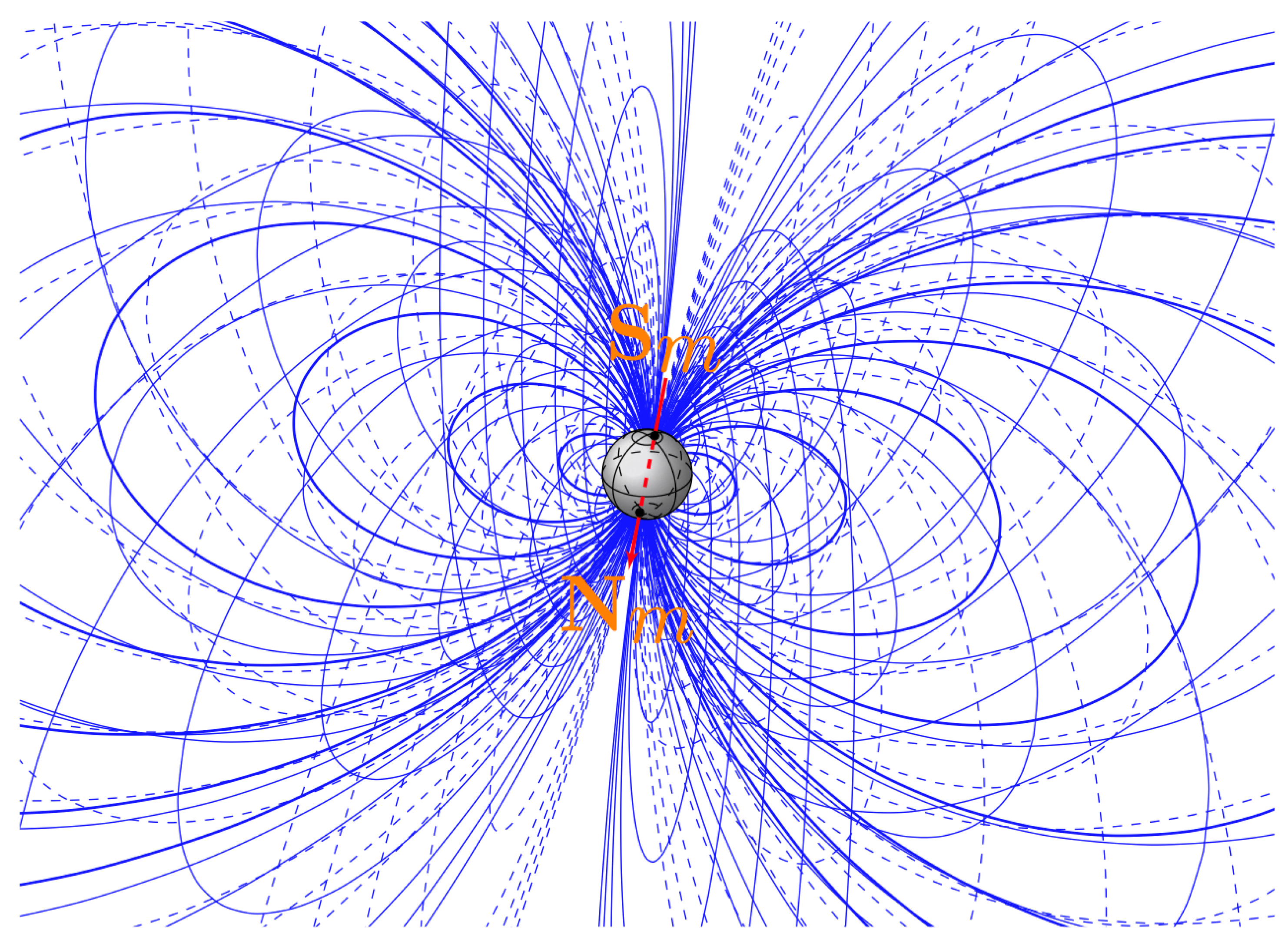
The geomagnetic field refers to the magnetic field that extends from the Earth’s interior into space and has the effect of a barrier against the charged particles carried by the solar winds. The magnetic field follows currents generated by convective motion caused by the heat escaping from the core of a mixture of molten iron and nickel in the Earth’s outer core. The size of the magnetic field at the Earth’s surface ranges from 25 to 65 T (T stands for Tesla) [21]. As shown in Figure 1, the north geomagnetic pole is located at the south pole of the Earth, and the south geomagnetic pole is located at the north pole of Earth. The magnetic axes of the two poles are tilted at approximately 11.3 degrees to the Earth’s rotation axis as if a giant bar magnet has been placed at this angle at the center of the Earth (red in Figure 1).
2.1. Geomagnetic Field Characteristics
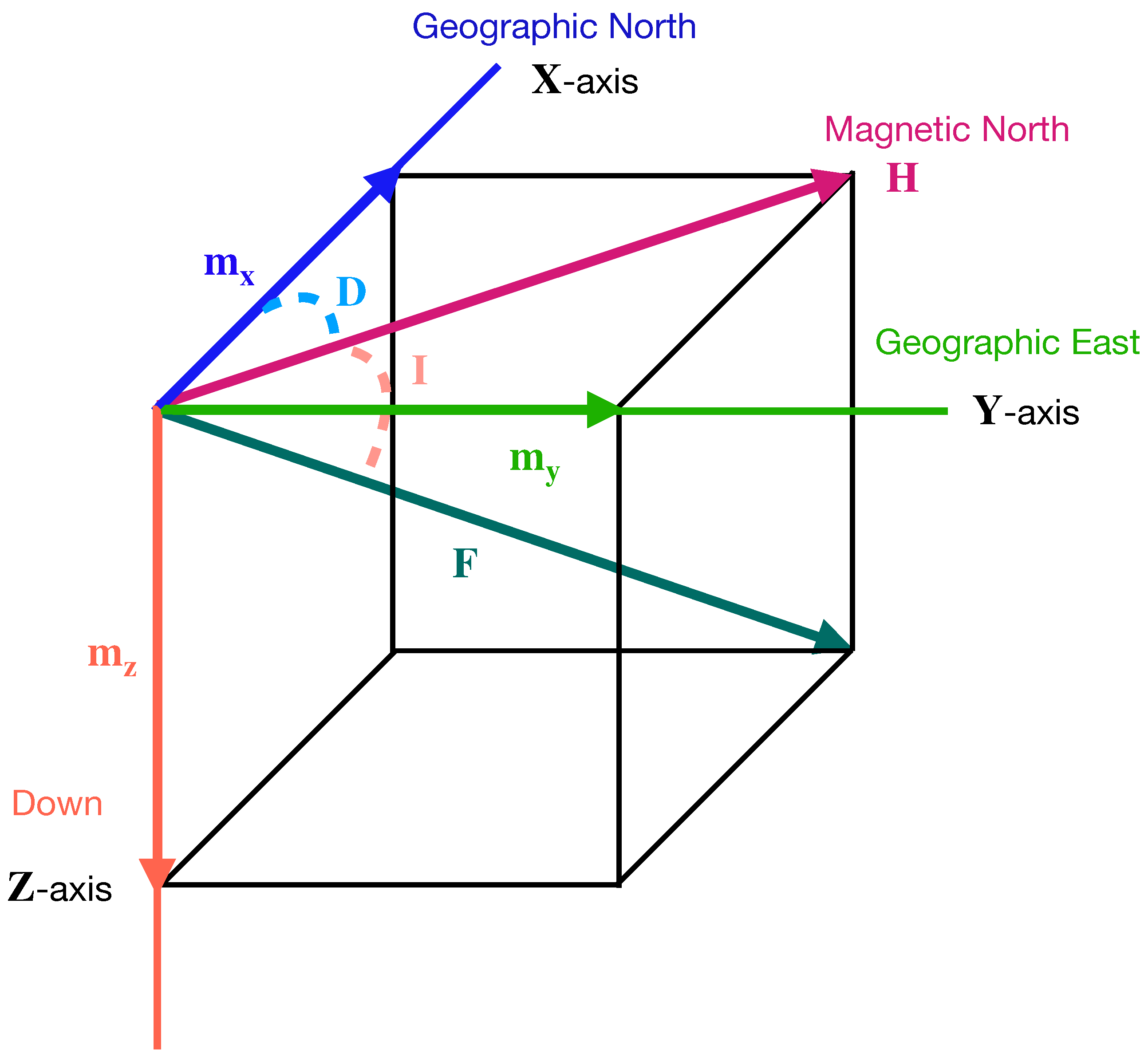
The geomagnetic field is a three-dimensional vector with three orthogonal magnetic field components: X, Y, and Z. It can be expressed by . Figure 2 illustrates the magnetic field vector, and H is the horizontal field component. The declination, D, is the angle between the geographic north and H. The inclination, I, is the angle between the total geomagnetic field intensity, F, and the horizontal plane [23,24].
For decades, researchers have known that homing pigeons, migrating birds, sea turtles, lobsters, and other species can somehow sense the Earth’s magnetic field to determine the direction they are traveling [25,26,27,28]. Spatial discrimination and temporal stability are two key characteristics that make up a good fingerprint [13,29,30]. In this section, we describe the geomagnetic field and summarize some of the characteristics of indoor magnetic field measurements—some of which are beneficial for indoor positioning, while others pose challenges for practical applications.
2.2. Advantages of Using Magnetic Field Measurement
Compared with WiFi [2], Bluetooth [3,4], ultrasound or sound [5,6], and visible light [7,8], magnetic field positioning has the advantages of temporal stability, uniqueness due to ferromagnetic disturbance, and tolerance to moving objects.
- Temporal stability: The temporal stability of the magnetic field measurement is an important characteristics. A lot of studies are reported in the literature on the temporal stability of magnetic field measurement [17,19,20,31,32,33]. The results of the current study show that magnetic field measurements are stable over time or vary slowly when no significant infrastructural changes are introduced in a given indoor environment.
- Uniqueness due to ferromagnetic disturbance: The ubiquitous magnetic field is disturbed by the ferromagnetic materials, such as steel or iron used in buildings, which distort the magnetic field measurements [17]. These disturbances cause the compass heading to fluctuate, resulting in incorrect direction and position information [34]. Haverinen et al. [13] collected indoor magnetic fields through the robot with embedded sensors indicating the presence of pillars, doors, and elevators in the room, making the magnetic field measurements more unique, so they can be utilized as a solution for indoor positioning. Subbu et al. [33] analyzed the cause for this uniqueness and then proposed a solution for indoor positioning by classifying the patterns of magnetic field measurements. Ashraf et al. [17] studied the effect of building materials on magnetic field data, provided a comprehensive analysis of the nature of the building, and discussed the variation of magnetic field disturbances.
- Tolerance to moving objects: The effect of moving objects, such as people or cabin, on the magnetic field is very limited and almost non-existent at a distance of 1 m. The authors of [31] studied the influence of moving objects, such as people, cabin, elevator, and electrical appliances, on the magnetic field in typical situations and showed that elevator infrastructure had a significant influence on the magnetic field measurement, whereas the moving cabin had little impact. Experiments given in [17] show that human mobility has no or a small effect on magnetic field measurements, and the addition of furniture in the indoor environment that does not contain ferromagnetic materials has no substantial impact on the magnetic field local signature. Since the signals in indoor environments are more complex than in outdoor environments. The reflection, diffraction, and scattering effects of wireless signals in media with different propagation characteristics (such as walls, floors, pedestrians, and other objects) can cause the attenuation of Wifi signals [35,36,37]. This highlights the huge advantages of magnetic positioning.
2.3. Challenges of Using Magnetic Field Measurement
The challenges of using magnetic fields for indoor localization mainly include the effects of low discernibility and smartphone heterogeneity, which affect the performance of localization.
- Low discernibility of magnetic field measurement: The magnetic field intensity at the Earth’s surface smoothly varies between 25 T and 65 T [21]. In a given indoor environment, the MF is affected by the local environment, leading to slight differences in the MF signature (measurement) at different indoor locations. However, almost identical magnetic field measurements might occur at different indoor locations, which leads to a low discernibility problem when using MF maps for the indoor location.
- Need for frame transformation: The geomagnetic vectors in the navigation frame and the smartphone frame are denoted as and , respectively. As the heading of the smartphone may be random in the coordinate navigation system, readings must be measured in different directions at each location [14], which is costly in terms of time and labor and prone to noise. In order to make the magnetic field measurements of the smartphones consistent, it is necessary to transform in the smartphone framework to in the navigation framework. However, the frame transformation process requires information from the gyroscope and accelerometer to obtain the rotation matrix, and it is a challenge to calculate the accurate rotation matrix.Suppose tilt information is available for the smartphone, we can use the [38] method to transform the geomagnetic field on the smartphone’s frame into the horizontal (denoted as ) and vertical (denoted as ) components [32]. After the transformation, the horizontal and vertical components are ’ideally’ independent of the user’s direction. Unfortunately, in practice, this is not the case because the accelerometer measurements (and hence the frame transformation) are affected during walking.
- Challenge with the use of MF intensity only: Note that, although the three-dimensional magnetic field measurements will be inconsistent when the smartphone is oriented differently, the magnetic field intensity is the same [33]. However, compared to using the MF vector , the magnetic field intensity is a scalar, which loses a large amount of information and can lead to a decrease in localization accuracy.Recent methods such as MaLoc [14] combine , , and to form a 3D vector for indoor localization. However, due to the , the 3D vector does not provide more information than the 2D measurement and therefore does not increase the localization performance.
- Heterogeneous Device: It is important to design a positioning method that can seamlessly integrate with the magnetic field of various smartphones. The major smartphone companies such as Apple, Samsung, Huawei, Xiaomi, etc., use embedded magnetometers from various manufacturers. There is no one standard for selecting embedded magnetometers for smartphones. The embedded magnetometer models used by the various smartphone companies have specific sensitivities and noise tolerances, resulting in their magnetic field measurements also varying. Table 1 shows the names and descriptions of the various magnetometers added to smartphones. Several major smartphone manufacturers have chosen different magnetometer models, and the sensitivity and operating temperature characteristics of these magnetometers are not exactly the same, resulting in different magnetic field measurement readings. Therefore, calibration is required before using the magnetometer. According to the Android documentation, rotating your smartphone in figure-of-eight swings calibrates the magnetometer measurement [39]. However, this simple calibration method does not meet the needs of magnetic field localization. The two main calibration methods mentioned in recent literature are ellipsoid fitting [40] and maximum likelihood estimation [41]. When the user walks indoors, the smartphone can obtain a geomagnetic measurement sequence, and the geomagnetic measurement sequence can improve the accuracy of positioning more than a single measurement [42,43]. Magnetic field sequence measurements show similarity between heterogeneous smartphones [17]. Using the Dynamic Time Warping (DTW) method, finding the minimum in the adjacent cumulative differences and calculating the cumulative distance is possible [44]. Variations in magnetic field data are caused by magnetic materials in the surrounding environment [10]. Smartphone calibration is required for each indoor environment in which positioning is performed.
3. Magnetometer Measurement Model
The magnetometer measures the magnetic field intensity along the sensor’s X, Y, and Z axes. The geomagnetic vector is a vector in navigation frame n aligned with the Earth’s gravity and the local magnetic field. Vector is in the sensor frame b. is a rotation matrix that indicates the transformation from the navigation frame n to the body frame b:
In an outdoor environment, the local geomagnetic field is equal to the local Earth’s magnetic field. Its horizontal component points to the magnetic north pole of the Earth [51]. The ratio between the horizontal and vertical components depends on its position on the Earth and can be expressed in terms of the inclination angle .
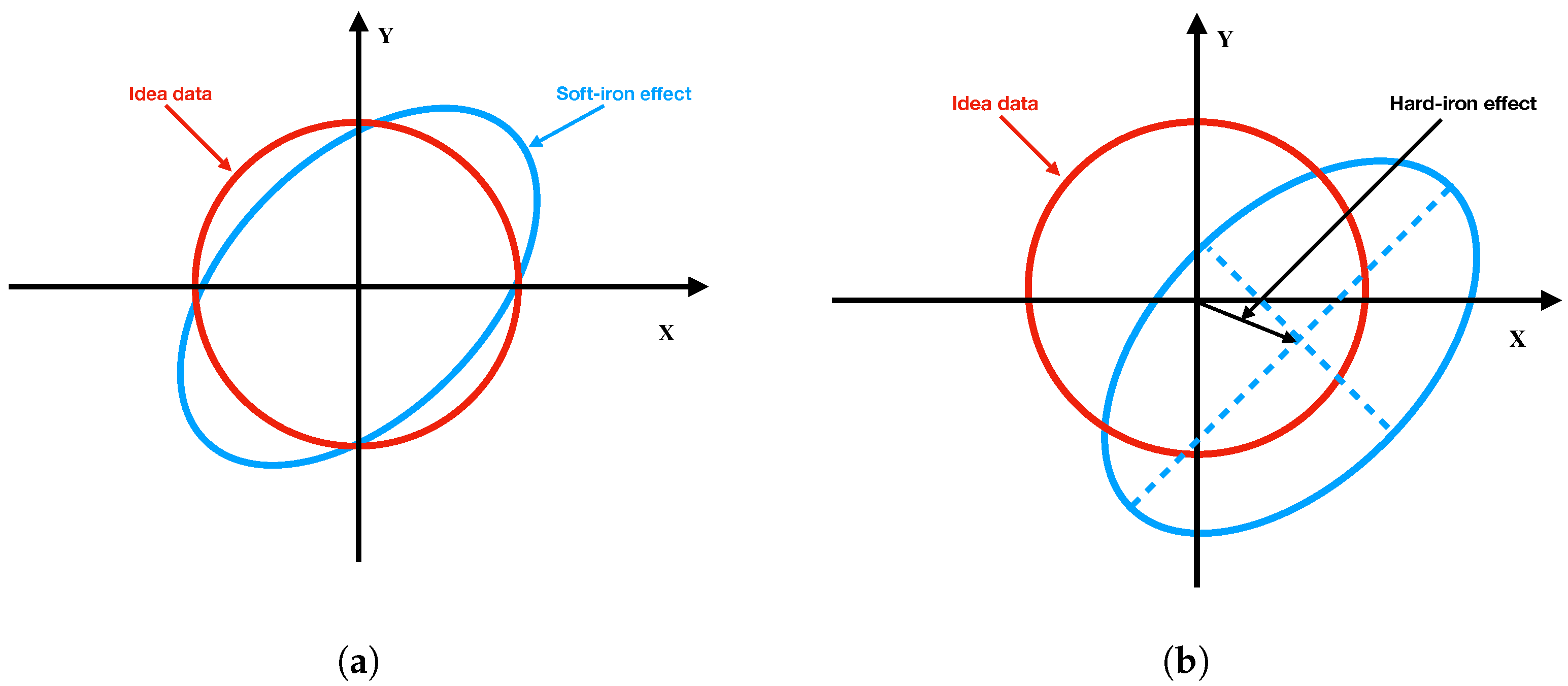
In the absence of any magnetic interference, rotating the magnetometer in all possible directions, the MF measurement is located on a sphere with a radius of the magnetic field intensity. However, indoor magnetic measurements may be affected by interference with the surrounding environment. Noise sources and instrument error degrade a magnetometer’s measurement. Noise sources result in two kinds of distortion. Metals such as nickel and iron could cause a soft iron effect, which distorts the sphere into an ellipsoid, as shown in the plot of Figure 3a. We model this distortion as . The hard iron effect is produced by materials that exhibit a constant additional field to the Earth’s magnetic field, as shown in Figure 3b. This distortion shifts the origin of the ideal magnetic measurement sphere.
With hard iron and soft iron effects, the magnetometer measurement model can be written as:
Instrumentation errors in magnetometers contain scale factors , misalignment errors , and sensor bias , which are unique and constant for a specific magnetometer [40]:
- The scale factor represents the difference in sensitivity of the three axes,where and denote the scale factor of sensors’ x, y, and z axis.
- The matrix indicates the misalignment errors of sensors which is given byin which and denote the error of sensor’s x, y, and z axis in the sensor frame, respectively.
- The vector shows the bias in sensors
Thus, the complete magnetometer measurement model is written as follows:
where is the local magnetic field, is the readings from the tri-axis magnetometers in the sensor frame. is an i.i.d Gaussian noise from . It is not necessary to identify all the components of Equation (10). Expanding Equation (10), the scale factor, misalignment, and soft iron distortion can be combined into a distortion matrix , and the hard iron effect and sensor bias can be formed into an offset vector .
The magnetometer measurement model can be expressed as:
4. Coordinate Systems and Transformations
There are several common coordinate systems used in inertial navigation. We summarize the coordinate systems in this section:
- The earth-centered earth-fixed (ECEF) coordinate system;
- The geodetic coordinate system;
- The local East-North-Up (ENU) coordinate system;
- The smartphone coordinate system;
- The 9 degrees of freedom sensor coordinate system.
The relationships among these coordinate systems and the coordinate transformations are also introduced.
4.1. Earth-Centered Earth-Fixed
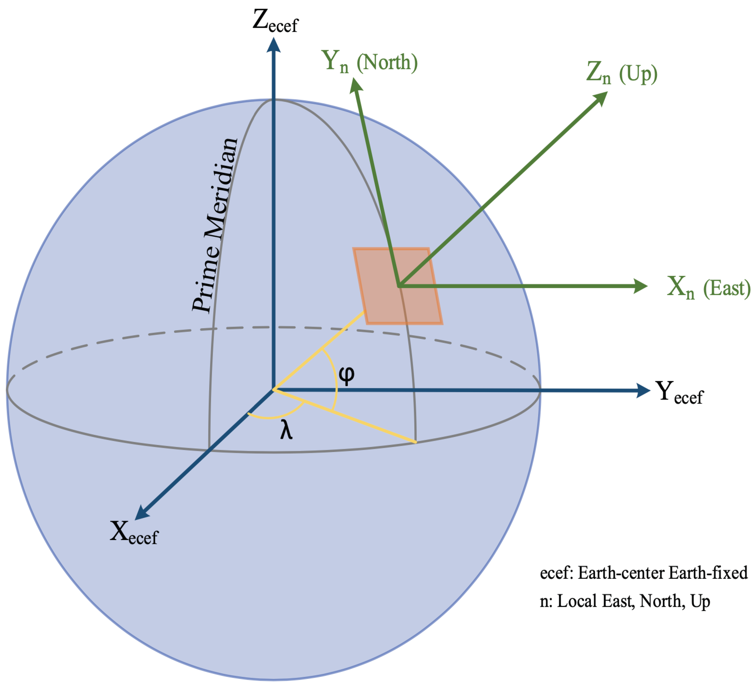
The Earth-Centered Earth-Fixed () coordinate system is a Cartesian coordinate system with the center of the earth as its origin, as shown in Figure 4. The X axis passes through the Equator and Prime Meridian intersection. The Z axis passes through the North Pole. The Y axis is orthogonal to X and Z. As a result, this coordinate system rotates with the earth. The distances used along each axis are meters. The position vector in the frame is denoted by
4.2. Geodetic Coordinate System
The geodetic coordinate system (see Figure 4) is widely used in GNSS-based navigation. It is a system that describes coordinate points close to the Earth’s surface in terms of latitude , longitude , and altitude h, respectively. Latitude measures the angle (ranging from −90° to 90°) between the equatorial plane and the normal to the reference ellipsoid passing through the point being measured. Longitude measures the angle of rotation between the principal meridian and the measured point (ranging from −180° to 180°). Altitude is the local vertical distance between the measured point and the reference ellipsoid.
The WGS 84 (World Geodetic System 1984) datum defines the Earth’s surface as an oblate ellipsoid with an equatorial radius a. An ellipsoid is a three-dimensional surface created by the rotation of an ellipse around its short axis. The shape of the ellipsoid can be described by the equatorial radius or semi-major axis a, the polar radius or semi-major axis b, the flattening f, and the first eccentricity squared e.
- Equatorial semi-major axis:
- Flattening:
- Polar semi-minor axis:
- First eccentricity squared:
the position vector in Geodetic coordinates could be denoted by
where represents the geodetic latitude, represents longitude, and h represents the ellipsoidal height, which can be converted into ECEF coordinates using the following Equation [52]:
where is the prime vertical radius of curvature defines as:
a and b are the equatorial radius (semi-major axis) and the polar radius (semi-minor axis), respectively. is the square of the first numerical eccentricity of the ellipsoid. The prime vertical radius of curvature N() is the distance from the surface to the Z-axis along the ellipsoid normal.
4.3. Local East-North-Up Coordinate System
The local ENU coordinate system is a coordinate frame fixed to the earth’s surface. Based on the WGS 84 ellipsoid model, its origin and axes are defined as shown in Figure 4: For a position vector that is given in ECEF coordinates, ENU coordinates can be transformed by multiplication with a rotation matrix.
4.4. Smartphone Coordinate System
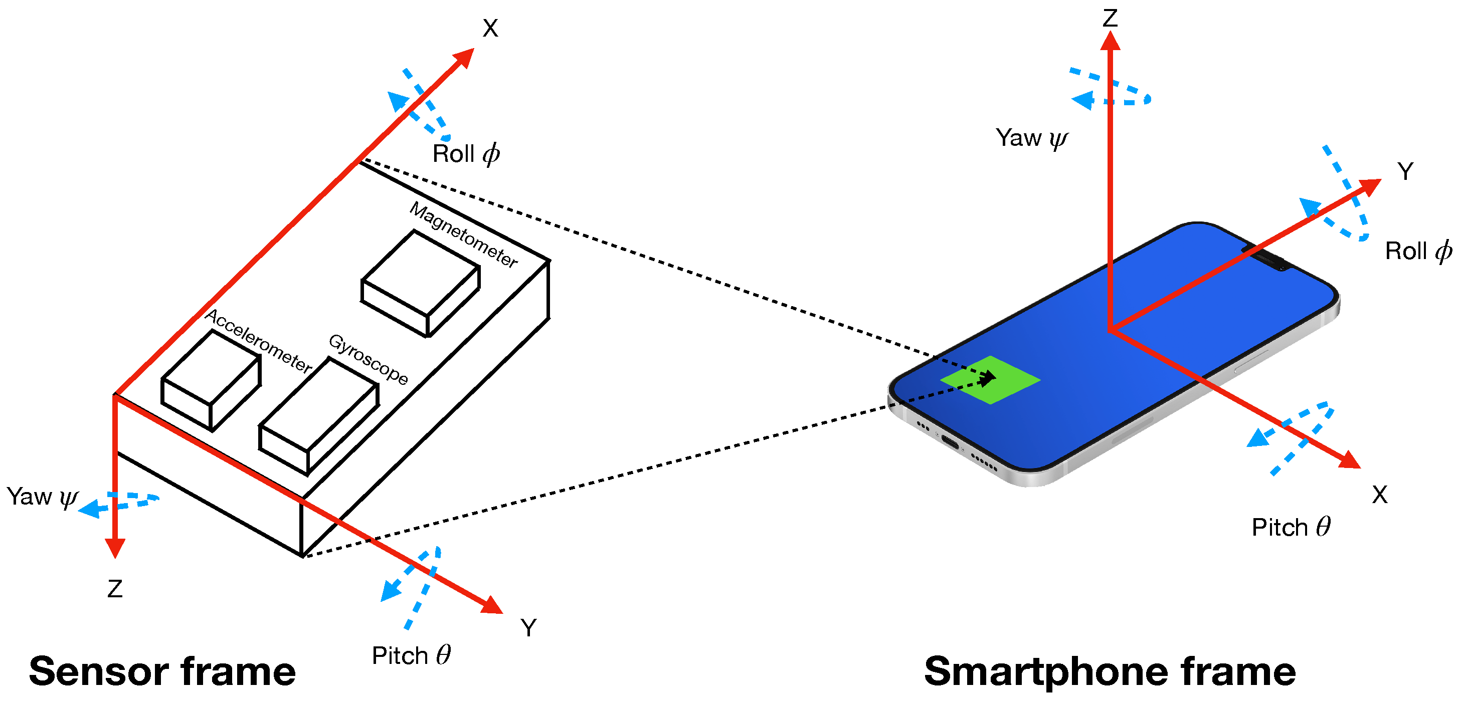
A standard smartphone coordinate system is shown on the right-hand side of Figure 5. X axis is horizontal and points to the right. Y axis is vertical, and Z axis points to the sky. Using a smartphone for mapping and real-time positioning usually does not require considering the transformation between sensor frames and device frames, but if you use an embedded robot for mapping and then use a smartphone for positioning, you need to consider the transformation relationship between the sensor frames and device frame. Figure 5 shows the transformation of the sensor frame to the smartphone frame.
4.5. Nine-DOF Sensor Coordinate System
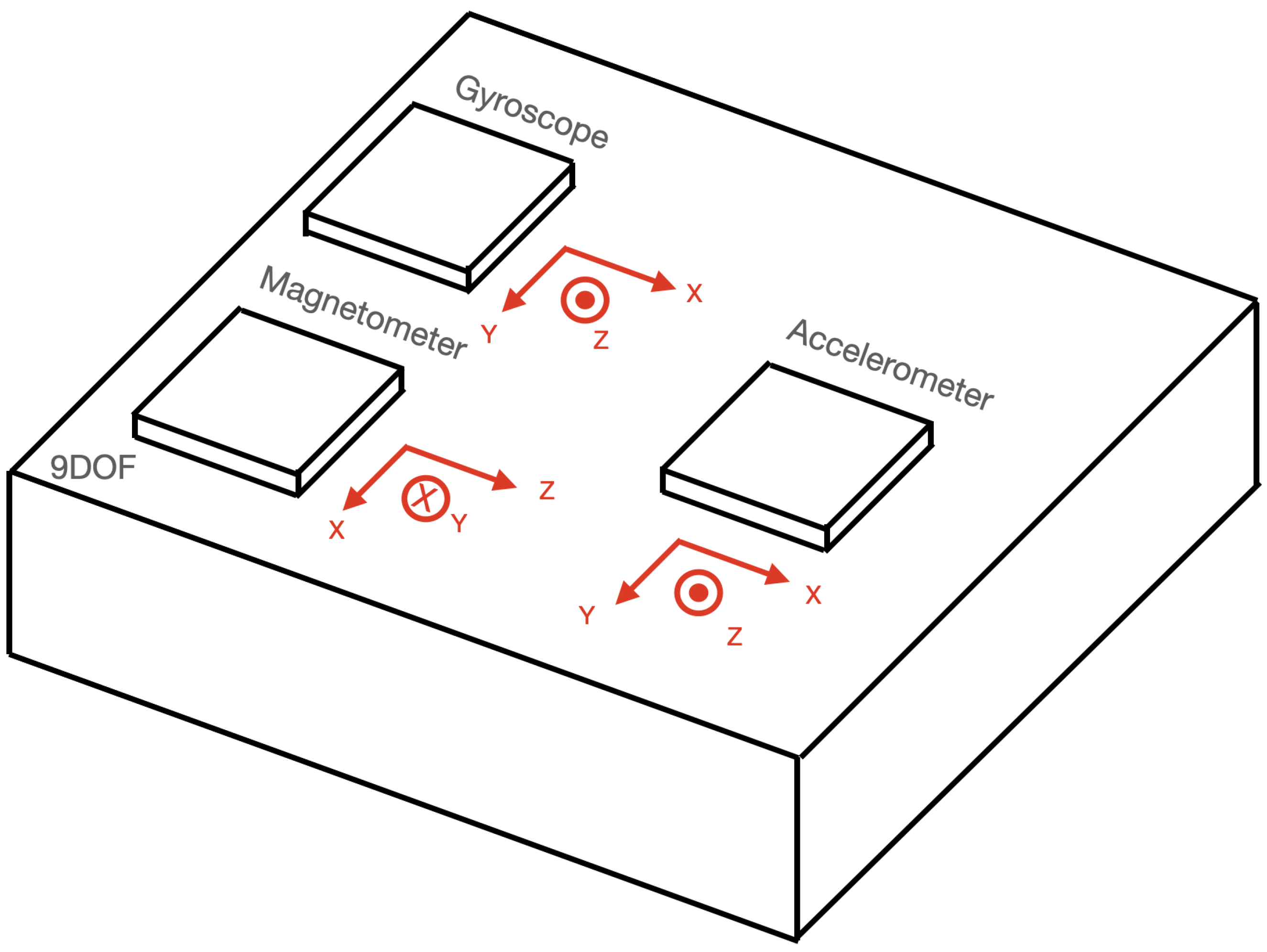
A sensor with nine degrees of freedom (9DOF) is often used in navigation robots (e.g., LSM9DS1), which contains a three-axis accelerometer, three-axis gyroscope, and three-axis magnetometer, but the coordinate systems of the accelerometer, gyroscope, and magnetometer are not the same. As shown in Figure 6, the coordinate systems of the accelerometer and gyroscope are the same, while the magnetometer is different from the other two, but they all have a left-hand rule relationship [53,54].
5. Magnetic Field Benchmark Datasets
Building geomagnetic databases are time-consuming and laborious, and it is significant to provide some publicly available geomagnetic databases for researchers to compare the state-of-the-art algorithms. However, there are some public magnetic field datasets for which the links are no longer available due to a lack of maintenance by the authors. This section presents several magnetic field datasets that are still accessible as of March 2022 and serve as a benchmark for many research papers.
- MagWi (accessed date: 7 March 2022) dataset was presented by [55] in 2021 It provides essential features of Wi-Fi and magnetic field data. Besides Wi-Fi and magnetic field, inertial measurement unit (IMU) data are provided from the accelerometer, motion sensors, and barometer involving four users, both male and female. The dataset can be used to study the effects of device heterogeneity, spatial diversity, smartphone orientation, walking speed, time-related mutations, and the impact of human movement on Wi-Fi and magnetic field measurements. Over nearly five years, the dataset was collected using five different smartphones, including Galaxy S8, LG G6, Galaxy A8, LG 7, and Galaxy S9+.
- UJIIndoorLoc-Mag (accessed date: 7 March 2022) dataset was presented at a 2015 international conference on indoor positioning and indoor navigation (IPIN) by [56]. The database was collected in a laboratory of approximately 15 × 20 m with eight corridors and 260 m of space. The sampling frequency was 10 Hz, and 54 different paths were selected for sampling. The sampling of each path was repeated five times so that the training set database consists of 270 different consecutive samples. There are also 11 test set databases. The test paths are complex, involving intersections and multiple turns. The information in the database includes Android’s magnetometer (TYPE_MAGNETIC_FIELD), accelerometer (TYPE_LINEAR_ACCELERATION), and orientation (TYPE_ORIENTATION) sensors. The smartphones tested were the Google Nexus 4 and the LG G3, with Android 5.0 as the operating system.
- Barsocchi et al. [57] dataset (accessed date: 7 March 2022) was presented at IPIN 2016. The dataset consists of 36,795 consecutive samples collected over an area of 185 m, including corridors and corridors connected by turns. The dataset includes data from Wi-Fi and magnetic fields, acceleration, and gyroscopes. Data collection was performed by wearing two devices simultaneously: a smartphone and a smartwatch. The smartphone model is a Sony Xperia M2, and the smartwatch model is an LG W110G Watch R.
- MagPIE (accessed date: 7 March 2022) was presented at IPIN in 2017 [58]. Data were collected by handheld and wheel-mounted robotic sensors over a test area of 960 m of floor space in three different buildings. The dataset also takes into consideration the changing and unchanging positions of objects that may affect the magnetometer measurements. The dataset includes data from magnetometers, accelerometers, and gyroscopes. Motorola Moto Z Play and Lenovo Phab 2 Pro were used for data collection.
- Miskolc IIS Hybrid IPS (accessed date: 7 March 2022) was presented at the 26th Conference Radioelektronika in 2016 in [59]. The dataset contains 1571 samples with 65 features. It covers three buildings (approximately 2000 m), which were divided into 22 zones. Data were collected using the Samsung Galaxy Young GT-S5360 with Android 4.4.4 version and sent to a server for processing and storage. Each sample includes information on 31 Wi-Fi access points, 22 Bluetooth devices, and 1 magnetometer with a unique location.
Table 2 summarises the publicly available datasets mentioned above. In addition to the datasets provided by the academic studies mentioned above, many publicly available datasets from indoor positioning competitions call on competitors to come up with positioning solutions to improve the entire indoor positioning field, e.g., Microsoft Indoor Localization Competition—IPSN 2016 Dataset and Indoor Location & Navigation—Kaggle DatasetWe can choose different datasets according to our needs. For example, if one needs to test the difference between a handheld smartphone or one mounted on a wheeled robot, one can select MagPIE; or if one needs to test the heterogeneity and orientation of a smartphone, one can choose MagWi, etc.
6. Magnetometer Calibration
Magnetometers are necessary auxiliary sensors for attitude estimation in low-cost, high-performance inertial navigation systems. The inexpensive, low-power magnetometers allow accurate attitude estimation by comparing magnetic field vector observations in body coordinates with magnetic field measurements in the Earth coordinate. The fusion of magnetometer and inertial sensor information leads to accurate 3D attitude estimation [60,61]. The accuracy of 3D attitude estimation is closely related to the calibration of the sensor measurements and the interference [62]. Magnetometers are more sensitive to environmental changes than inertial sensors and require more frequent recalibration [41]. The calibration of magnetometers could be divided into two methods: attitude-dependent and attitude-independent.
The classical compass swing calibration method presented in [63] is a heading calibration algorithm that requires leveling and an external known heading source and keeps the magnetometer plane level. This method is attitude-dependent.
In recent years, attitude-independent calibration methods have been explored in the literature. The TWOSTEP batch method was proposed in [64] to estimate magnetometers’ bias with an unknown attitude. In the first step of the algorithm, the initial predictions of the calibration parameters are obtained by a centering approximation method to solve the resulting quadratic objective function. The second step estimates the parameters by a batch Gaussian–Newton iterative estimation method system. Crassidis et al. [65] compared three recursive magnetometer calibration algorithms: the sequential centering algorithm, the extended Kalman filter (EKF), and the Unscented filter (UF). Among them, the sequential centering algorithm is a linear least-squares method based on the centering approximation. The experimental results show that the EKF and UF algorithms have smaller residual magnitudes and mean residuals closer to zero than the sequential centering algorithm. The UF algorithm is more robust than the other two algorithms in terms of accuracy and convergence properties.
The goal of the calibration method is to estimate the calibration parameters A and b in Equation (13). The batch magnetometer calibration method uses the entire set of magnetic field measurements to estimate the unknown calibration parameters [66], using an attitude-independent observation to estimate the magnetometer error term. This observation is derived from the fact that the magnetometer measurements are constant and independent of the attitude of the local measurement position [67]. The cost function is constructed from the difference between the measurement model of the magnetometer and the true geomagnetic measurements. The calibration parameters are estimated with the maximum likelihood method. In [68], the calibration is considered a parametric optimization problem formulated through maximum likelihood estimation (MLE), and the optimization algorithm is derived using the gradient and Newton descent method. The sensor alignment matrix is obtained through the solution of the orthogonal Procrustes problem. The initial conditions of the iterative algorithm are obtained with suboptimal batch least-squares calculations. Approximate MLEs are sensitive to initial errors, and inaccurate initial estimates can lead to magnetometer calibration failure. Wu et al. [67] proposed an optimal MLE magnetometer calibration algorithm based on a quadratic method. Compared with the approximate MLE method, the optimal MLE calibration has advantages in terms of accuracy and stability, but the computational cost of the optimal MLE calibration is relatively high. Kok and Schön in [41] transformed the calibration algorithm into a maximum likelihood problem by using ellipsoid fitting to obtain the initial values of the calibration parameters, then using the extended Kalman filter (EKF) to calculate the rotation matrix and the accumulated errors, and finally constructing the cost function. References [69,70] proposed a particle swarm optimization (PSO) algorithm to solve the parameter estimation problem in magnetometer calibration. PSO is a global optimization algorithm that transforms the calibration problem into a parameter optimization problem. The PSO-based calibration algorithm has the advantages of no initial values and linearization, easy implementation, and fast convergence. Classical iterative solutions are based on the approximation of the gradient to find the minimum of the cost function. Tahir et al. [71] transformed the magnetometer calibration model into a stochastic optimization problem using a modified simultaneous perturbation stochastic approximation (SPSA) method for gradient estimation, giving similar calibration results to the PSO-based method but with much less computational complexity. These methods were implemented by minimizing the difference between the measured magnetic field and the local reference magnetic field [72], which was denoted as scalar checking. The scalar checking methods assume that the local magnetic field is stable during calibration and rotate the measured magnetic field to an arbitrary direction to minimize a certain scalar cost function. However, the scalar checking method for magnetometer calibration has the problem of rotational ambiguity. The calibration model in Equation (13) conforms to the ellipsoidal limit, and the calibration matrix cannot be fully determined because the ellipsoidal parameters are fewer than the calibration model parameters. To explain the rotational ambiguity problem from mathematical principles, the calibration matrices derived from the ellipsoid coefficient matrix by different matrix decomposition methods are not unique, and there exists an unknown rotation matrix between them [73].
Table 3 summarises mentioned calibration algorithms’ accuracy, robustness, computational cost, and deployment difficulty.
The deployment of magnetometer calibration algorithms needs to consider device dependencies, smartphone heading, and the effects of environmental noise. Smartphone battery consumption is closely related to the complexity of the magnetometer calibration algorithm.
7. Magnetic Field Map Construction
Indoor maps are a prerequisite for indoor positioning systems. Hiring experts to build indoor maps and update them regularly is an expensive and time-consuming method that cannot be applied to large-scale indoor coverage. In recent years, researchers have proposed some crowdsourcing and SLAM-based methods to construct indoor floor plans [74]. Unlike traditional expert site surveys, crowdsourcing is an approach that uses crowd contributions to achieve complex tasks and is well suited for fingerprint-based indoor locations [75].
7.1. Traditional Map Survey
He et al. [31] proposed a compliant-walking-based site survey method: the surveyor places the smartphone in a fixed body position and walks along a pre-planned measurement path from the starting point to the endpoint. The smartphone records the accelerometer, gyroscope, and magnetometer readings during the walk. The estimated actual user trajectory is matched to the pre-planned path to determine the location of each step. The positions of the collected magnetic signals are interpolated from the positions of adjacent steps.
7.2. Crowdsourcing Approaches
Crowdsourcing-based localization systems typically have lower localization accuracy than the systems based on explicitly surveyed fingerprint data. Table 4 depicts the comparison of localization accuracy based on geomagnetic field crowdsourcing methods. Mobile crowdsourcing methods do not require pre-labeled reference points and manual calibration and are becoming an attractive way to construct magnetic field maps [76]. When building fingerprint databases using crowdsourcing approaches, location estimates from the PDR method are often used as the location labels for the measurement data [77]. MeshMap is an indoor positioning system based on magnetic fields and crowdsourcing [78]. A magnetic fingerprint database is constructed by merging sensor data from different paths of multiple users using a crowdsourcing approach. In order to combine magnetic navigation maps, a dynamic time warping-based matching algorithm is developed for map stitching, overlapping region checking, magnetic field time series matching, and position correction. A cubic spline interpolation algorithm is used for the purpose of robustness. It is reported that 70% of the time, the navigation error is within 2 m, and 95% of the time, it is within 4 m. The accuracy of the dead reckoning method is affected by the accumulation of errors due to sensor noise, and the accuracy of the constructed floor plans of indoor paths usually inferred from only one dead reckoning trajectory is low. Luo et al. [74] proposed a crowdsourcing method to collect data from magnetometers, gyroscopes, and accelerometers in smartphone. Magnetic anomalies caused by magnetic materials in modern buildings were applied to the system as a unique index. PDR techniques, magnetometer measurement models, and trajectory fusion based on affinity propagation algorithms are used. Magnetic trajectory data were clustered using dynamic time-warped similarity criteria. It is reported that an indoor map with an accuracy of 0.48 m was successfully constructed. Ayanoglu et al. [79] proposed an automatic FingerPrinting (FP) map construction algorithm based on many user trajectories. This crowdsourced approach utilizes only the inertial sensors of mobile devices and does not require specialized infrastructure or floor plan information. Overlapping of multiple user trajectories can be identified by clustering magnetic field measurements and heading features at the detected turns. These clusters are used as landmarks in the map construction process, and the trajectory information between the landmarks can iteratively update the locations of the landmarks.
7.3. Mapping with Simultaneous Localization and Mapping
PFSurvey was proposed in [80] for the rapid creation of signal maps that could be used to survey an entire building in a matter of minutes. The method uses accelerometer, gyroscope, and magnetometer data to estimate the surveyor’s trajectory and uses SLAM and particle filters to incorporate a floor plan of the building, achieving trajectories within 1.1 m of ground truth in 90% of the time. Compared to maps generated by traditional time-consuming manual surveys, PFSurvey’s data collection costs are lower, but it achieves similar accuracy.
7.4. Geomagnetic Field Interpolation
Interpolation is a technique for adding new data points to a set of known data points and is commonly used to fill in missing magnetic field data in indoor positioning algorithms based on magnetic field positioning. Suppose the user’s location is within the localization area, but the magnetic field data are missing at that point. The magnetic field measurement can be computed using the magnetic field data points close to the query point.
The Gaussian Process (GP) is a powerful nonlinear interpolation method, and many standard interpolation methods are equivalent to a specific Gaussian process. Assume that the geomagnetic field can be modeled by three independent Gaussian processes [81], and then the model is generalized as a multivariate normal distribution given by
where is the mean vector, and is the covariance function given by
where is a variance hyperparameter, and is a length scale hyperparameter. and represent two different points on the continuous domain of the Gaussian process; is the distance between and ; the output of function represents the covariance value between the Gaussian distribution represented by and —the larger the distance, the smaller the correlation between the two distributions.
Vallivaara et al. [82] proposed a simultaneous localization and mapping (SLAM) method based on local anomalies of an ambient magnetic field using a Rao-Blackwellized particle filter to estimate the pose distribution of the robot and a Gaussian process regression to simulate the magnetic field map. This method demonstrated that geometrically consistent magnetic field maps can be generated using odometer and magnetic field measurements. However, this work was only tested in a small area, and based on this, Akai and Ozaki [83] used a mobile robot to collect magnetic data and efficiently built large-scale magnetic maps using GP. Wahlström et al. [84] introduced a Bayesian nonparametric model based on a vector-valued stationary Gaussian process to estimate the magnetic field and the magnetic source jointly. The divergence and curl-free properties of the magnetic field from electromagnetic theory were exploited to calculate its covariance function. Solin et al. [85] presented a Bayesian nonparametric probabilistic modeling approach for the interpolation and extrapolation of magnetic fields. By imposing a GP on the potential scalar of the magnetic field, the magnetic field components are jointly modeled using Maxwell’s equations, providing a model for the ambient magnetic field that allows continuously updating the estimates and the time variation of the magnetic field. Kok et al. [86] combined the physical properties of the magnetic field with a Gaussian process model to represent the magnetic field map and uses three-dimensional hexagonal block maps to create local maps. Reduced-grade Gaussian process regression combined with Rao-Blackwellized particle filters make the computation tractable. The approach provides a scalable magnetic field SLAM algorithm for computational complexity and map storage.
8. Indoor Localization Methods Using Magnetic Fingerprints
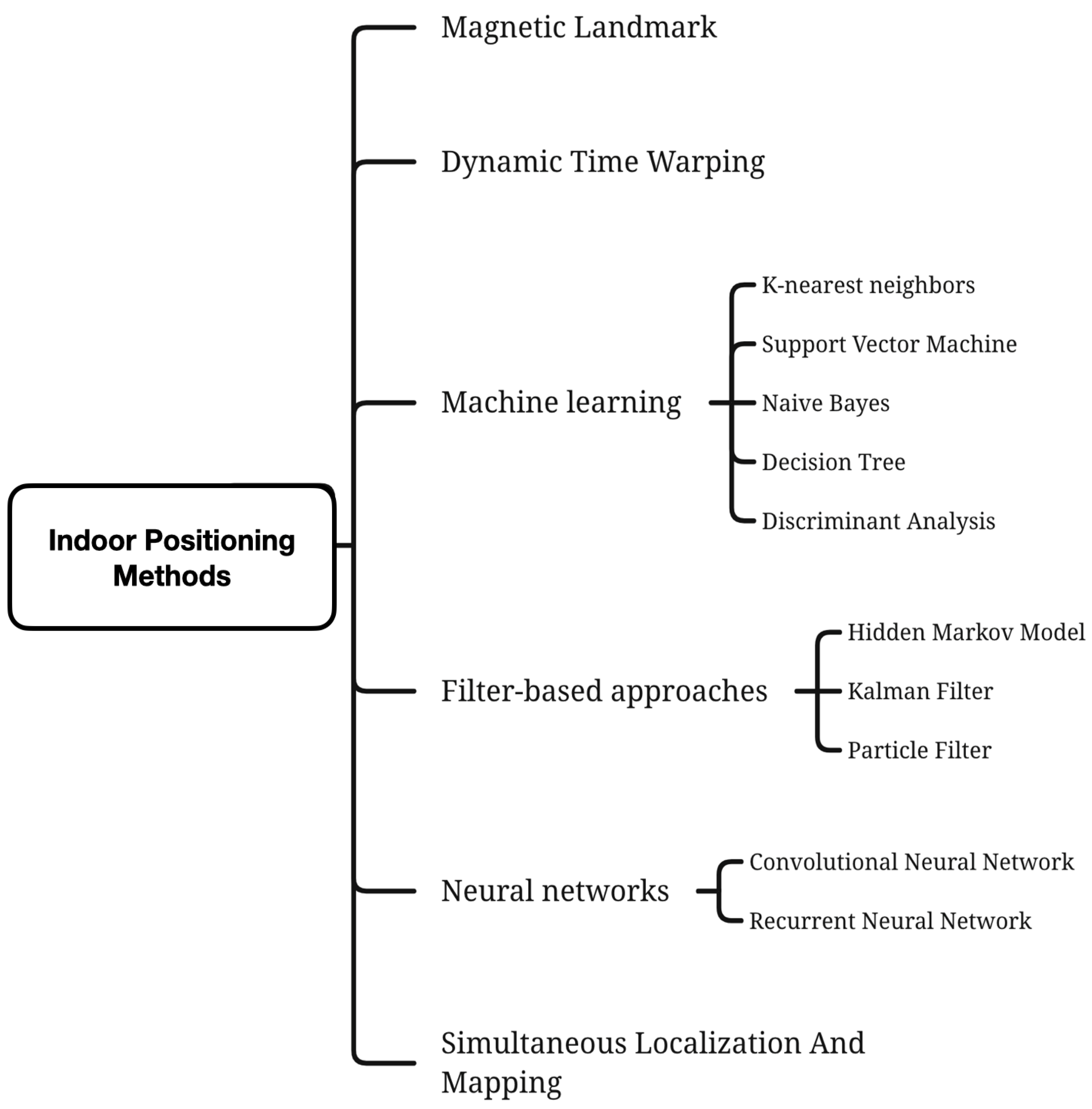
Fingerprinting is a common location method that works by matching fingerprint measurements to fingerprints in a database to estimate the location of an object. The accuracy of magnetic fingerprint localization can be affected by smartphone orientation and environmental changes. In addition, magnetic field localization accuracy depends on fingerprint density, and the acquisition and maintenance of high-quality magnetic maps is a time-consuming and labor-intensive process [87]. Compared with other methods, it has relatively low complexity and high applicability in complex indoor environments [2]. Fingerprinting consists of two phases: training and offline [88]. In the training phase, a fingerprint database of a certain granularity is built in the region of interest. The finer the granularity, the higher the accuracy, while the time and labor costs increase. In the offline phase, the collected measurements are matched with the fingerprints in the database using deterministic algorithms or probabilistic algorithms [18] to calculate the location of the object. There are some popular magnetic fingerprinting-based positioning algorithms using pattern recognition techniques. Figure 7 summarizes the research on indoor localization based on magnetic field fingerprinting, and we will follow this scheme to discuss magnetic-field-based localization methods. This section will first discuss how local geomagnetic anomalies of landmarks can be used to determine target locations in Section 8.1. We then discuss how to use dynamic time warping for position matching in Section 8.2. We next examine machine-learning-based magnetic fingerprinting methods in Section 8.3. Then, we discuss filter-based methods for magnetic field localization in Section 8.4. We then discuss the magnetic field localization with Simultaneous Localization and Mapping in Section 8.5. Finally, we discuss the application of (deep) neural networks to magnetic field localization in Section 8.6.
8.1. Magnetic Landmark
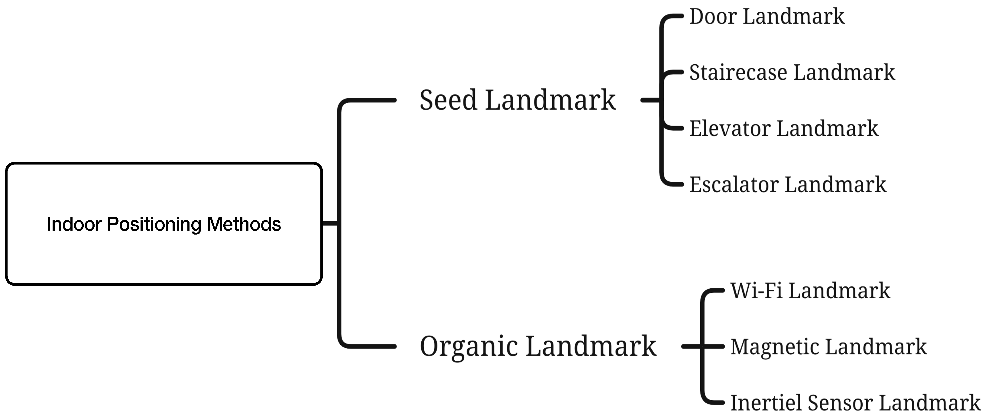
Landmarks are defined as location points in indoor environments where at least one type of sensor data presents a distinctive, stable, and identifiable pattern [89,90,91]. The survey [92] provides a comprehensive review of landmarks localization methods. Landmarks can be categorized as seed landmarks and organic landmarks [89,90], as shown in Figure 8. Seed landmarks correspond to landmarks at physical points in the environment, including stairs, lifts, escalators, etc. Seed landmarks have a unique impact on one or more mobile phone sensors and can be uniquely detected. Organic landmarks (such as WiFi landmarks, magnetic landmarks, and inertial sensor landmarks) do not correspond to specific objects and are usually detected based on their unique signature on the sensor [90].
Devices, such as fridges, lifts, metal doors, etc., can make the magnetometer readings show prominent variations and be used as magnetic landmarks. Magnetic landmarks can be used to enhance indoor positioning and mapping [89,90,93], to detect indoor/outdoor environments [94], and to label the semantics of indoor environments [95]. There are several research works that utilize landmarks to enhance indoor localization. An early system using landmarks for indoor localization is UnLoc [89], which achieves a median localization error of 1.69 m by combining PDR with landmarks. SemanticSLAM [90] further extends the UnLoc system using the SLAM technique, which decreases the median localization error to 0.53 m. An activity landmark-based indoor mapping system is presented in [96], which is called ALIMC. By detecting the activity landmarks, ALIMC achieves a mapping accuracy of about 0.8–1.5 m within the 80th percentile. APFiLoc [93] uses a particle filter to fuse PDR, landmarks, and a floor plan, which achieves a localization accuracy of less than 2 m with 80% confidence. Specific methods for identifying seed landmarks are presented in [97]. For example, turns can be identified using angle- or direction-dependent sensors. Lifts can be easily identified based on unique patterns of vertical acceleration data. The acceleration pattern of taking the escalator is similar to a stationary state. The acceleration pattern for going up or down the stairs is similar to regular walking. The door landmarks contain two phases of acceleration: the low value of opening the door and the periodic pattern of walking out. Subbu et al. [33] distinguished corridors with success using magnetic signatures resulting from different components or sources of interference in the room, such as pillars, doors, and lifts. Landmark-based localization also has some limitations. Firstly, landmark detection. Existing work typically involves manually designing detection features and setting thresholds for detecting different landmarks through empirical analysis, which may vary from scene to scene. There is no general method to learn useful landmark detection features automatically. Secondly, the problem of data association is to be considered, i.e., determining the correct landmark when there are multiple landmarks nearby. Thirdly, the omission problem, i.e., certain landmarks, may be missed in some cases. For example, a door landmark can be missed if the door is open because most door detection methods assume that the user performs a series of activities while passing through the door (e.g., walking-standing and opening the door-walking) [98].
8.2. Dynamic Time Warping
Dynamic Time Warping (DTW) has many applications in magnetic field localization by compressing or stretching the time axis of one (or both) magnetic field sequence(s) to align two magnetic field sequences with similar patterns but with differences in amplitude and time. Subbu et al. [44] used DTW to classify magnetic signatures collected from different corridors. By aligning unknown magnetic signatures with known signatures, the technique can obtain a close match between test and specific magnetic signatures that vary in time, thus providing the correct corridor/location information. Wang et al. [77] used backward magnetic fingerprints synthesized from magnetic fingerprints collected online in the forward direction to improve localization accuracy. Assessed through the DTW that the synthetic backward magnetic trajectories were similar to the actual backward magnetic observations. In this way, we can obtain more magnetic trajectories for localization. Li et al. [99] proposed a localization method (CSMS) that integrates channel state information (CSI) and magnetic field strength (MFS). The CSMS constructs an integrated fingerprint map of CSI and MFS. The initial localization coordinates are first obtained according to the M-KNN algorithm in the localization phase. Then, the Local Dynamic Time Warping algorithm is applied to match the geomagnetic sequence during the motion for tracking. Finally, according to the tracking position, the Multi-Module Data k-Nearest Neighbor algorithm dynamically weighs the multi-module data to narrow down the localization range and perform fingerprint matching to obtain more accurate localization results. DTW usually calculates the distance between the measured magnetic field and the magnetic fingerprint in the database. Based on the traditional DTW, Chen et al. [100] proposed an improved DTW (3DDTW) that extends the one-dimensional input signal into a two-dimensional one. Then, 3DDTW was used to calculate the distance between the measured magnetic field and the magnetic fingerprint, thus reducing the mismatch of the magnetic fingerprint. Finally, weighted least squares were used to reduce indoor positioning errors with a hybrid positioning accuracy of approximately 3.3 m.
8.3. Machine Learning Approaches
With the development of artificial intelligence, machine-learning-based indoor positioning is becoming a trend, and machine learning algorithms can effectively address many of the limitations of traditional positioning techniques for indoor environments. The most important advantage of the machine learning approach is its ability to learn helpful information from input data with known or unknown statistics [101].
In machine-learning-based localization, classifier algorithms such as K-NN [102], support vector machines (SVM) [103], naive Bayes [104], decision trees [105], and discriminant analysis [106] are widely used to extract the core features of a signal. Localization methods need to consider accuracy and computational complexity, and acquiring high-dimensional data through feature engineering to improve accuracy can introduce high computational complexity. Dimensionality reduction techniques such as principal component analysis (PCA) [107] and singular value decomposition (SVD) [108] techniques can transform high-dimensional features into low-dimensional ones, significantly reducing the storage space and computational complexity of magnetic fingerprint-based localization.
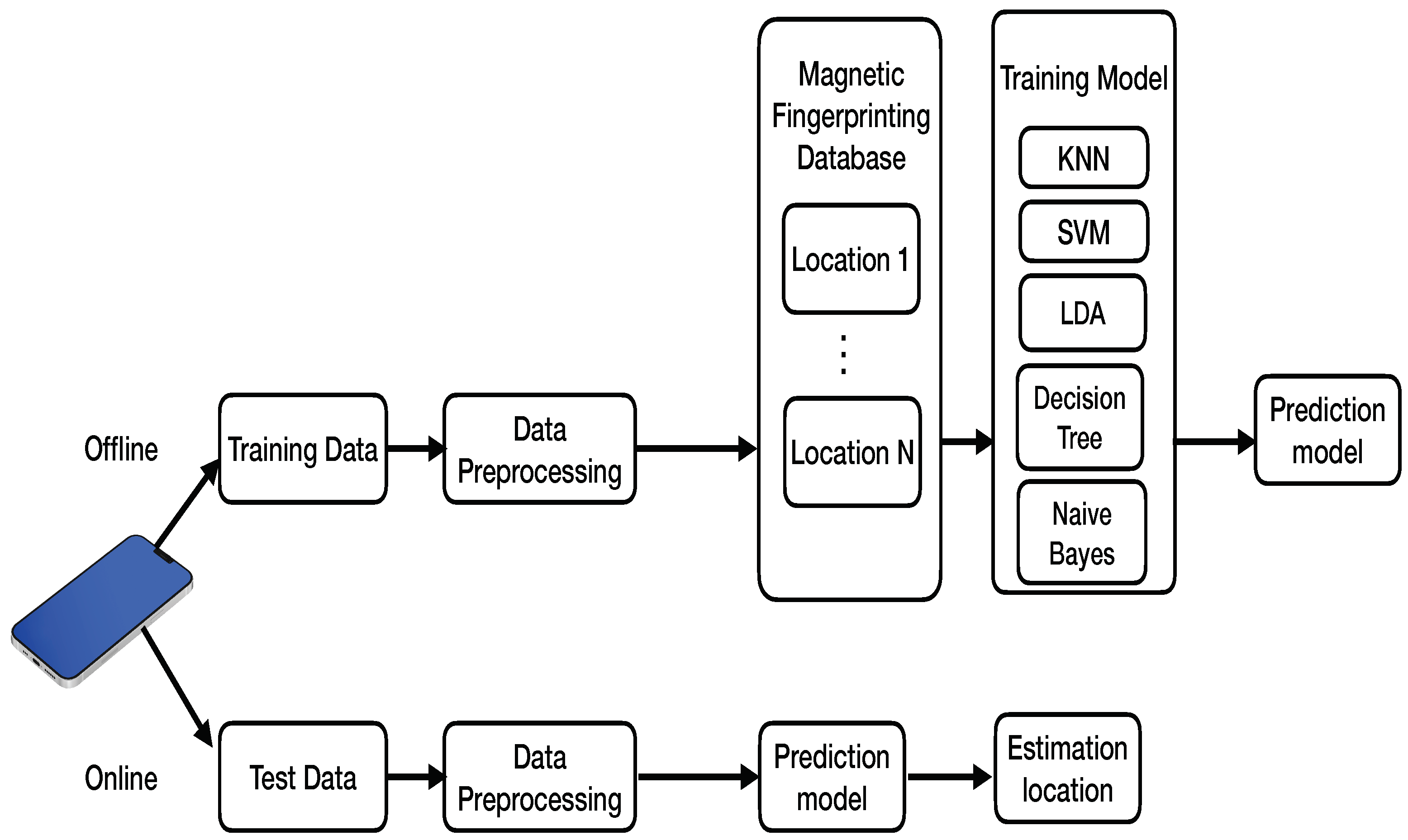
The architecture of a magnetic-based positioning system is shown in Figure 9. The system consists of two phases: online and offline. First, raw magnetic data are collected at a reference location using a smartphone. Then, during pre-processing, low-pass filters, smoothing filters, and calibration algorithms are applied to remove noise and bias from the smartphone’s magnetic measurements. Subsequently, the combined pre-processed data generates a fingerprint database corresponding to each location. The fingerprint database is trained using machine learning methods (e.g., kNN, support vector machines, decision trees, naive Bayes, discriminant analysis) to obtain predictive models. Finally, a prediction model is used to predict the test data’s position. We will focus on fuzzy kNN, support vector machines, decision trees, naive Bayes, and discriminant analysis in the following.
Fuzzy K-nearest neighbor: Fuzzy K-nearest neighbor algorithm [109] is a well-known algorithm for classification. The theory of fuzzy sets was introduced into the k-nearest neighbor technique to develop a fuzzy version of this algorithm called fuzzy-k-nearest neighbor. Not only does the fuzzy algorithm have the advantage of a lower error rate, but the resulting membership also provides a confidence level in the classification. Fuzzy-k-nearest neighbor was shown to perform well compared to other more complex classification algorithms. The principle of the algorithm is to assign membership as a function of the Euclidean distance vector from the basic k-nearest neighbor algorithm and memberships in the possible classes.
The algorithm is defined as follows: Given a location of magnetic training set, collected from n points in the test area with m features. The second magnetic test set contains, from n points. We compute the metric
where , in which k is number of nearest neighbors, and , in which n is the number of points. The fuzzy parameter m is used to determine the weights of the distances. Here, we set .
Decision tree: A decision tree is a non-parametric supervised learning technique consisting of multiple decision rules, all of which are derived from data features. In a decision tree, we call the whole sample the root node, and the process of dividing a node into two or more sub-nodes is called splitting. When a sub-node splits into more sub-nodes, it is called a decision node. Nodes that do not split are called leaves. The process of deleting the sub-nodes of a decision node is called pruning. The decision tree algorithm splits the training set (root node) into subsets, recursively splitting until no pure sub-nodes (leaf nodes) are obtained. The decision tree algorithm requires optimal attributes and thresholds that maximize the splitting criteria (e.g., CART Tree), and the resulting set of splits is optimal. Commonly used decision tree models such as the CART algorithm use Gini’s impurity index, the ID3 algorithm uses Information Gain, and the C4.5 algorithm uses Gain Ratio [105].
Naive Bayes: The Naive Bayes classifier is based on Bayes’ theorem. Suppose has n samples with m features, class labels . According to Bayes’ rule, can be expressed as
where and are known. To estimate the location, we need to find the corresponding location that maximizes . Since the magnetic values obey a Gaussian distribution, i.e., , and are derived from the training set [104].
Discriminant analysis: Discriminant analysis methods are well known for learning discriminative feature transformations and can be easily extended to multiple class cases [110]. Suppose we have training data , n samples with m features, class labels . The within-class scatter matrix given as:
where and is the number of samples in . The between-class scatter matrix equation is defined as
where is the number of training samples for each class, is the mean for each class, and is total mean vector given by . The Fisher criterion suggests that the linear transformation maximizes the ratio of the determinant of the between-class scatter matrix of the projected samples to the within-class scatter matrix of the projected samples [106].
The transformation can be obtained by solving the generalized eigenvalue problem [110]:
Support vector machine: Support vector machine classifies data by finding the best hyperplane, which is the hyperplane with the maximum distance between two classes. Given n samples of training data with m features, labels . The i-th SVM is trained using all examples with positive labels in the i-th class and all other examples with negative labels, and the i-th SVM is formulated as follows:
where the training data are mapped to a higher dimensional space by a function f, is a vector representing the direction of the separated hyperplane, is a constant representing the position of the hyperplane, C is the penalty parameter that defines the trade-off between large separation regions and misclassification errors, and is slack variable that allows some samples to be on the wrong side of the separation hyperplane [111,112,113].
After solving Equation (31), there are the decision functions:
x belongs to the class with the largest value of the decision function.
K-NN is widely used for pattern-matching magnetic fingerprinting. However, K-NN has poor performance in handling large datasets and high-dimensional datasets. Fingerprinting approaches such as support vector machines [114] and linear discriminant analysis [115] have been shown to improve localization accuracy while increasing the computational cost. The main challenge of deterministic methods is that although some sampling points are spatially close, their magnetic field similarities are farther apart, leading to significant localization errors. Huang et al. address this problem using the multidimensional scaling (MDS) method in [116]. Support vector machine employs a kernel mechanism to find the differences between two classes, modeling linear and nonlinear relationships with better generalization and effectively handling large datasets and high-dimensional datasets [117]. However, SVM-based methods are computationally complex and require significant time and memory when the number of support vectors becomes large. Decision-tree-based indoor localization has shown good performance in improving localization accuracy [118]. The disadvantage of decision trees is the possibility of missing information when processing and classifying continuous numerical data.
8.4. Filter-Based Approaches
Filter-based methods are usually applied to fuse data from multiple sensors to provide high accuracy for indoor solutions. The localization system state is often not directly available, and the localization system state is usually estimated from a system measurement model and a motion model. Mathematically, these two models can be represented as follows:
where k is the timestamp, is the system state for time k, is the state-dependent equation of motion, is the state-dependent equation of measurement, is the measurement (i.e., magnetic field), and and represent process noise and measurement noise, respectively.
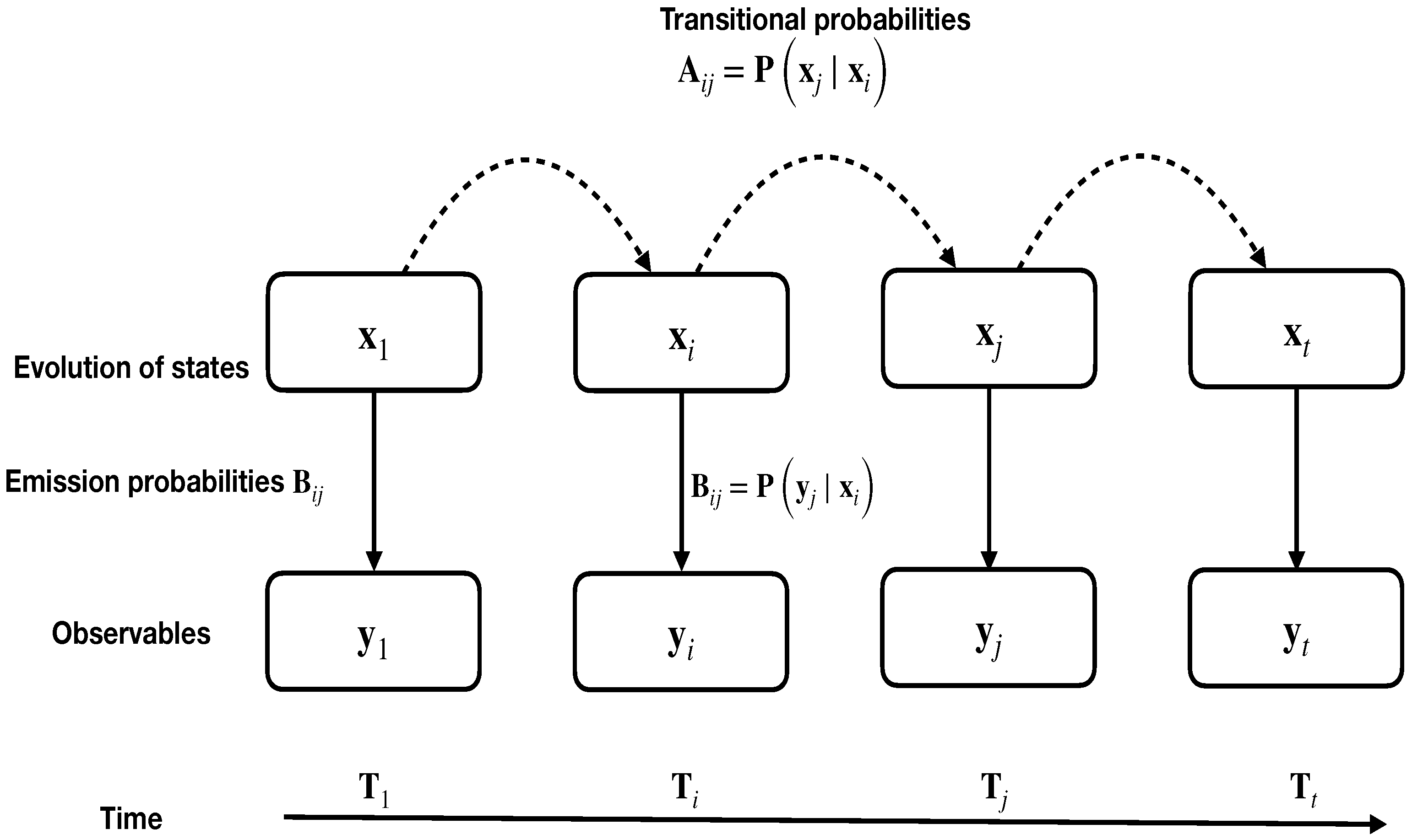
Hidden Markov Model: A Hidden Markov Model (HMM) is a statistical Markov model in which the system (hidden state) is assumed to be a Markov process. The HMM assumes the existence of another process that depends on and can be learned by observing . As shown in Figure 10, a typical Hidden Markov Model is described by a state-space model. Formally, the HMM model is characterized by five parameters:
- is a set of N hidden states. The state at time i is denoted by , representing the k-th real position;
- is a set of M observations. Magnetic signal observation sequences at time i are denoted by ;
- is the transition probability matrix, where denotes the transition probability from state to state ,
- is the emission probability matrix, where indicates the emission probability at time j from state ,
- is the initial state distribution. If there is no prior knowledge about the initial state of smartphone, the vector ,
HMM addresses three main types of problems:
Evaluation problem: Knowing the model parameters , and the observed sequence , calculate the probability of occurrence of the observed sequence.
Prediction problem (also called the decoding problem): The model’s parameters are known, and the sequence of observations and the most likely states sequence corresponding to the observations sequence is calculated.
Learning problem: Model parameters is not known, inferring model parameters.
In magnetic field positioning, we use the k-th hidden state of the HMM to denote the user’s position after step k. There is a special conditional probability distribution for geomagnetic field intensity observations called the emission probability distribution. A complete HMM consists of the initial probability, the transition probabilities, and the emission probabilities. Usually, the initial probability is known. The transition probability is calculated by pedestrian dead reckoning (PDR). The emission probability is the probability of observing the geomagnetic intensity in state . The HMM then generates observations at each state through the emission probabilities. Ma et al. [119] proposed Basmag, a HMM-based indoor localization system using a Backward Sequence Matching Algorithm (BSMA) to optimize the HMM and improve the low discriminability of the geomagnetic signal with the help of PDR. Kwak et al. [120] presented an unsupervised learning algorithm based on HMM and designed a lightweight algorithm to compare the similarity of magnetic fingerprints. It is reported that the matching learning accuracy is 96.47%, and the positioning median error is 0.25 m. The Kalman filter or extended Kalman filter applies to Gaussian distributions and cannot be applied to non-Gaussian signals. HMM is more computationally efficient than particle filters of high complexity. Compared to other Bayesian filtering techniques, HMM is more suitable for representing the complex motion of indoor targets [121,122].
Kalman filter: Kalman filter principle is well described in [123,124,125]. Assume that f is a linear function with respect to and and h is a linear function with respect to and , then Equation (33) can be rewritten as:
where and are zero-mean white Gaussian noise and independent of each other.
The covariances of and are, respectively, and . The process and measurement matrices and , and the noise parameters , are time variables. The covariance matrix is updated between measurement steps:
, where and are the mean and covariance matrix of , respectively, the correction equation for the measurement update is:
The Kalman gain matrix is calculated for each update:
Zhao and Wang [126] showed that the use of EKF could reduce the cumulative error of inertial sensors and improve the accuracy of orientation and position measurements. Wang et al. [127] fused information obtained from the PDR and the magnetic fingerprint with EKF and PF schemes. It demonstrated higher localization performance than using PF alone.
In a positioning system, the system state or user state is the user’s position and orientation.
Assuming that the user’s motion is considered to be on a horizontal plane (2D), we can obtain the acceleration and orientation from the accelerometer and gyroscope in the smartphone. The relationship between these sensor measurements and the user’s state is as follows, and Equation (38) can be rewritten as:
where l is the step size, is the user’s change in heading between two consecutive steps, and and are Gaussian noise.
In the measurement model, we use the magnetic fingerprint as the primary observation . Equation (39) is used to obtain the observations for state in the fingerprint database.
The initial values of the system state and the covariance matrix are set, and the parameters of the process noise and the measurement noise are obtained from the sensor measurements. A Kalman-filter-based positioning system is complete.
Particle filter: A particle filter is a Sequential Importance Sampling (SIS) method that expresses the state distribution of an object by extracting random state particles from the posterior probabilities. Each particle has a corresponding weight that represents the value of the function at the point determined by that particle. The greater the number of particles, the more approximate the desired distribution function.
In particle filters, the state of the object of interest is usually represented by the vector . We may be interested in the user’s position and velocity during localization. Therefore, we can represent each state by a vector containing the position and user velocity. The prior probability function represents a roughly calculated value of the following possible state, given that we have information about its current state (dynamics). After the observation, the weights of the particles are updated to form the posterior probability function , which represents the probability of updating the particle when is observed.
To estimate the next state, we only need to resample the weighted particles, preserving the size of the particle set. In the prediction step, the weights of each new particle are adjusted according to the motion dynamics model with random errors. The function represented by the new set of particles is then considered as the new prior function for the next step [128,129].
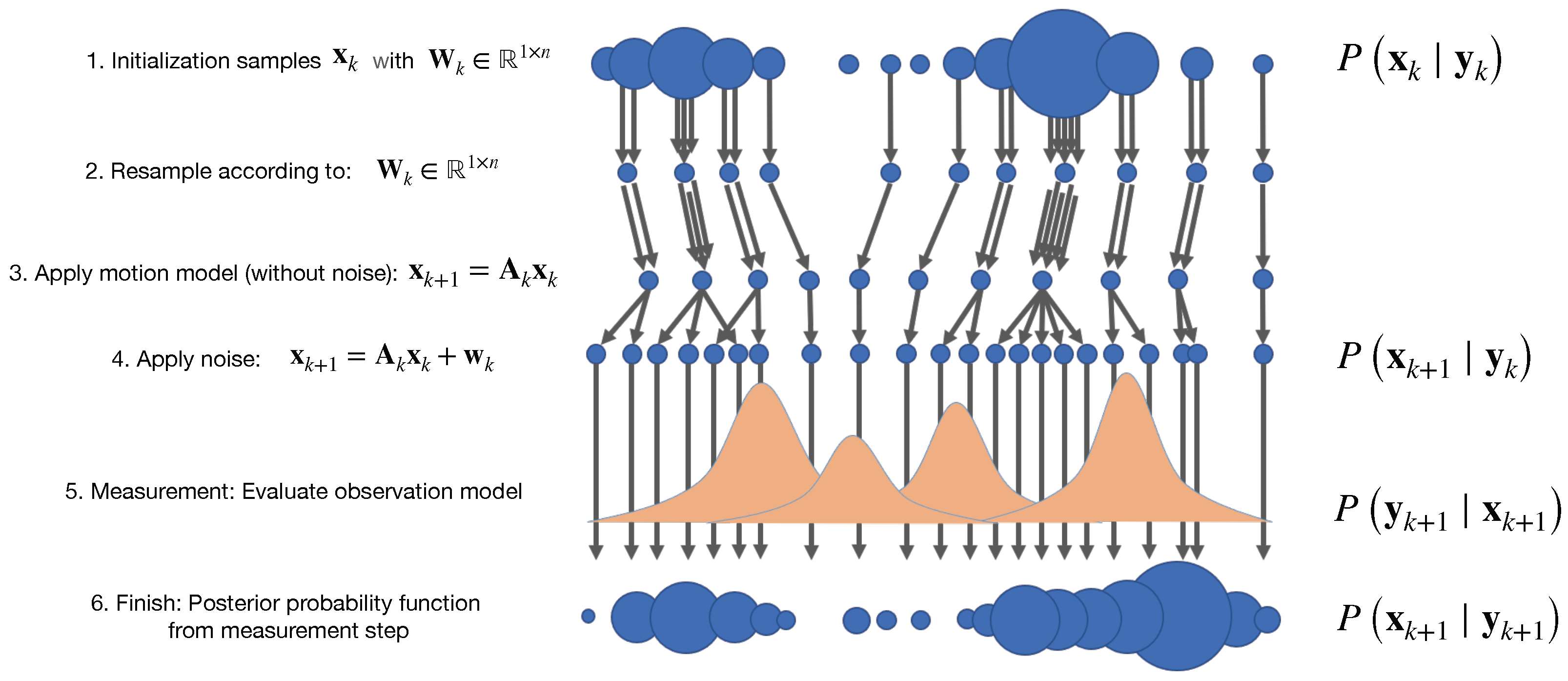
Figure 11 illustrates a particle filter loop.
Layer 1: In the first layer, we have particles represented by circles of different sizes, indicating the importance of a particle .
Layer 2: The second layer illustrates the resampling process, where particles are resampled according to their weights, and particles with higher weights have a higher chance of being selected. The same particle can be selected multiple times—resampling. When a single sample has extremely dominant weights, the resampling step is necessary for degeneracy. After the particles are resampled, the weight distribution is set to be uniform.
Layer 3: The motion process of the particles shown in the third layer is predicted to be different since each particle has a different state after applying the model .
Layer 4: Noise is applied to cover some unlikely assumptions and distinguish the particles if some of them are the same—the resampling step.
Layer 5: After obtaining the noise measurements, the observation model is evaluated based on the state estimates of each particle. The observation model assumes the probability that the measurement will occur when we know the state of the object. Layer 6: The sixth layer shows the posterior probability function resulting from the measurement step. Applying the observation model to each particle, particles whose observations are similar to actual ones will have greater weights. In contrast, particles distant from the actual observations will receive low weights. Finally, the updated particles are used to evaluate the state (e.g., median or mean of the particle states) for the next iteration.
We now describe how the particle filter actually works. First, N random particles are generated from an initial region . A particle is an assumption about the state of the user with a weight.
where is the weight of the particle. The motion model for each particle is updated with Equation (46). The probability of observing on state is given as
where n is the dimension of , is the covariance matrix, and is a function to obtain observations of state in the fingerprint database. We evaluate each particle by
Finally, we use the weighted average of the current particles to estimate the true state, as shown in Equation (50).
The particle filtering approach has specific applications in magnetic field localization. For example, Xie et al. [130] innovated the motion, measurement, and resampling models for smartphone indoor localization systems and proposed a reliability-augmented particle filter. They used a dynamic step estimation algorithm and a heuristic particle resampling algorithm to reduce the error of motion estimation and improve the robustness of the elementary particle filter. The use of combined PF and EKF is proposed in [127] to fuse the information obtained from PDR and magnetic fingerprinting and to improve the inherent blindness in the traditional PF scheme and solve the particle degradation problem. This fusion algorithm has a localization accuracy of 1–2 m in large buildings when the user walks slowly, which has a higher accuracy compared to many other algorithms.
8.5. Simultaneous Localization and Mapping
Simultaneous localization and mapping (SLAM) uses both mapping and localization algorithms to build a map and simultaneously localize objects within that map. Many researchers have recently combined SLAM with smartphone sensor data for location estimation, as summarized in Table 5. Wang et al. [131] introduced eSLAM, a simultaneous localization and mapping (SLAM) method that utilizes measurements of the ambient magnetic field present in all indoor environments. They implemented a modified exponentially weighted particle filter to estimate objects’ pose distribution and a Kriging interpolation method to update the magnetic field map. Through simulations on Matlab and tests on mobile devices, they observed two interesting phenomena: the shift in position estimation after sharp turns and the cumulative error.
Besides this, there are two main challenges for SLAM based on magnetic field measurement. The first one is that map construction for large-scale indoor environments is a difficult task. The second one is that the continuous data exchange between the map and the localization algorithm consumes a lot of power. Vallivaara et al. in [82] proposed a SLAM method using the local anomalies of the ambient magnetic field. A Rao-Blackwell particle filter was implemented for the pose distribution estimation of the robot, and Gaussian process regression was used for magnetic field map modeling. MagSLAM was presented in [132], and it demonstrated that simultaneous localization and mapping of indoor pedestrians using measurements of ambient magnetic field strength and human stride measurements without using an a priori map built by ground truth-based methods could be scalable and accurate. The work in [86] combines reduced-rank Gaussian process regression and Rao-Blackwellized particle filter to provide a scalable 3D magnetic field SLAM algorithm. It shows the feasibility of using smartphone measurements to obtain accurate position and orientation estimates. SemanticSLAM [90] is a calibration-free indoor positioning system that utilizes unique signatures of specific locations in an indoor environment. Unique signatures include unique patterns in the smartphone’s accelerometer when climbing stairs, unusual magnetic interference in specific locations, as well as unique Wi-Fi access on others locations. SemanticSLAM used these unique signatures as landmarks and combined them with a pedestrian dead reckoning in the (SLAM) framework to reduce localization errors and convergence times. It shows a median positioning error of 0.53 m with fast convergence times.
8.6. Neural Networks MF-Based Methods
There have been many studies on magnetic field localization methods based on an artificial neural network (ANN), and ANN is often applied for classification and prediction. For magnetic-field-based localization, the NN is trained using the magnetic field measurements and the corresponding position coordinates obtained in the offline phase. Once the ANN is trained, it can estimate its location based on the online magnetic field measurements. The existing ANN-based methods for magnetic-field-based localization are mainly a convolutional neural network (CNN) and a recurrent neural network (RNN). CNN usually converts magnetic field fingerprints into ‘image patterns’ for classification and RNN for magnetic field time sequence prediction. Table 6 summarizes the deep-learning-based approach to magnetic field localization.
DeepPositioning is a deep-learning-based indoor fingerprinting solution that combines magnetic field and WiFi fingerprinting with a deep neural network model to improve the accuracy of indoor localization [133]. While DeepPositioning is computationally expensive in the training phase, it is lightweight in the testing phase, which is advantageous for achieving real-time indoor localization on mobile devices. The performance of DeepPositioning depends on the number of APs (access points), RPs (reference points), and labeled samples in the training dataset.
Ashraf et al. [134] presented a multi-sensor indoor localization method using magnetic field measurements from a smartphone magnetometer and images from a camera to construct a database. A deep-learning-based convolutional neural network (CNN) classifier was used for scene recognition to narrow the search space of the database. Considering the similarity of magnetic signatures and the spatial proximity of the selected candidates, a modified K-nearest neighbor (mKNN) was proposed to compute the current location of pedestrians to improve the accuracy of localization. An extended Kalman filter was also implemented to further optimize the location estimation from the pedestrian dead reckoning data. This method is reported to be able to locate a person within 1.08 m 50% of the time for any smartphone used for localization. This represents a solution to the magnetic field localization method for heterogeneous smartphones.
MINLOC [135] proposed using a Magnetic Pattern (MP) and CNN for indoor localization. The MP generated at the measurement point is used to construct a database. The trained CNN is used to calculate the location. A voting mechanism is designed to vote on the predictions of multiple CNNs to estimate the user’s current location indoors. The method does not require knowledge of the user’s starting location and investigates the effect of various user heights on the localization performance. The results show that the localization accuracy of MINLOC is within 1.01 m 75% of the time, taking into account the heterogeneous smartphone and user height. This method performs better than the other two methods, mPILOT [19] and GUIDE [20].
Sun et al. [136] proposed a hybrid localization method based on Bluetooth RSS (received signal strength) and magnetic field measurement data. The method converts the Bluetooth signal strength data in the fingerprint library into a ‘fingerprint image’ and then uses CNN for fingerprint localization. First, the CNN is used to classify the floor by the received Bluetooth signal strength, and the classification accuracy of floor location reaches 96.7%. After the floor was classified, the real-time magnetic field measurement data were matched with the magnetic field data in the area database to calculate the coordinates of the unknown point. The test accuracy reached 93.33%, with a positioning error of fewer than 1.4 m. When using a CNN for the dynamic localization test, the classification accuracy exceeds 91%, and the accuracy of dynamic localization is also within 1.55 m. This convolutional-neural-network-based fingerprint localization method provides a new solution for multi-floor large indoor environments.
DeepML is a system based on deep long and short-term memory (LSTM) [137]. It uses the magnetic and light sensors of a smartphone for indoor localization. Bimodal images were built by preprocessing, and location features are extracted by a trained deep LSTM network. Finally, an improved probabilistic approach is leveraged to estimate the smartphone’s location. The experimental results showed that about 58% of the test locations had a position error of less than 0.5 m, and 82% had a position error of less than or equal to 2 m in the laboratory. In the corridor, 65% of the test locations had a position estimation error less than or equal to 0.4 m. A total of 87% of the test locations achieved an error of 3 m or less.
RNN was introduced to predict the position of geomagnetic signal sequences generated when objects move [138,139,140,141]. A recurrent neural network (RNN) is a deep neural network model identifying time-varying data sequences. RNN combines current input data with remembered previous data sequences to produce output results from its recurrent network model. According to the test results, the geomagnetic field signal localization based on the LSTM model has a localization accuracy of 0.51 m in a medium-scale testbed and 1.04 m in a large-scale testbed. The average localization errors of the basic RNN model were 1.20 m and 4.10 m, respectively, [138].
The work in [141] mentioned that despite having the same magnetic field measurements at multiple locations, the spatial/temporal sequence of magnetic field values around a particular region would form a unique pattern over time. Therefore, an LSTM deep recurrent neural network (DRNN) is proposed for learning magnetic patterns from spatial/temporal sequences. The experimental results show that the overall classification accuracy of the DRNN model is 97.20%, which is better than traditional machine learning methods, such as support vector machines and K-nearest neighbors.
Neural networks are promising in complex environmental scenarios where feature extraction is high and there is challenging data dimensionality [142]. Neural networks allow for analyzing large amounts of unlabeled and unclassified data. Its most significant advantage is automatically extracting features from the acquired data without manual extraction [143]. Indoor positioning is often faced with global positioning errors and kidnapping robot problems. When the initial position is unknown, this is known as the global localization problem. An RNN estimates the next position by predicting a time series and can be an excellent solution to this challenge.

Table 6.
Comparison on NN-based localization methods.
| Papers | Information | Method | Area | Device | Accuracy |
|---|---|---|---|---|---|
| DeepPositioning [133] | Magnetic field, WiFi | DNN | 13.4 × 6.4 m | Huawei MT7-TL00 | 60% of test samples under 1.5 m, 78% of test samples under 2.0 m |
| Ashraf et al. [134] | Camera magnetic field | CNN mKNN | 9720 m | Galaxy S8 and LG G6 | 50% of the time within 1.08 m |
| MINLOC [135] | Magnetic field | CNN | 1 building with 92 × 34 m, 1 building 28 × 44 m. | Samsung Galaxy S8 for training data and Galaxy S8 and LG G6 for testing. | 75% of the time within 1.01 m |
| Sun et al. [136] | Bluetooth, magnetic field | CNN | 1059.84 m | Nokia X7 | dynamic positioning within 1.55 m |
| Bae and Choi [138] | Magnetic field | LSTM | 94.4 × 26 m and 608.6 × 49.3 m | Samsung Galaxy S8 | 0.51 and 1.04 m for the medium and the large-scale testbeds, respectively |
| DeepML [137] | Magnetic field, light sensors | deep LSTM | 6 × 12 m Lab, 2.4 × 20 m corridor | Samsung Galaxy S7 Edge | 58% of error less than 0.5 m, 82% less than 2 m in Lab 65% of error less than 0.4 m and 87% less than 3 m in corridor |
| Bhattarai et al. [141] | Magnetic Landmark | LSTM-based DRNN | 100 × 2.5 m and 7 × 7 m | Android smartphone | 97.20% accuracy |
9. Smartphone-Based Pedestrian Dead Reckoning
Inertial navigation is an infrastructure-free method that uses inertial sensor measurements (accelerometers and gyroscopes) on the pedestrian to track the position and orientation of the object relative to a known starting point [144,145].
Inertial navigation technologies are divided into strapdown inertial navigation system (SINS) and pedestrian dead reckoning (PDR).
SINS binds one or more Inertial Measurement Units (IMUs) on the human body (such as head, waist, legs, feet, etc.), utilizes the mechanical equation to calculate the location of pedestrian, and employs Zero Velocity Update (ZUPT) to reset the integration errors [87]. PDR calculates walking steps and estimates step length and moving direction based on the smartphone-embedded IMUs to reckon the position of pedestrian. The challenge with PDR-based methods is the accurate heading estimation for the user, which is especially difficult when the user is carrying the device in any position. Moreover, both PDR and SINS approaches suffer from the drift problem (i.e., small errors in the measurement of acceleration and angular velocity which are integrated into progressively larger errors in trajectory estimation), which makes it unsuitable for long-term localization.
The fusion of PDR/SINS and magnetic fingerprint localization can mitigate this problem and achieve better localization accuracy than a single magnetic fingerprinting localization method.
9.1. Step Detection
Recent literature has proposed using the camera [146] and gyroscope data [147] for step counting, and we focus here on step counting with a built-in accelerometer for smartphones.
Time domain approaches: Time-domain methods can be divided into thresholding [148], peak detection [149], zero-crossing [150], and auto-correlation [151,152,153].
- Threshold: The threshold method calculates the number of steps by determining whether the sensor data meet some predetermined threshold. The work in [154,155] proposed a relative threshold detection scheme. It uses acceleration measurements already projected into the vertical direction to detect steps. The scheme detects a step when a valid maximum peak (as a maximum value) and a valid minimum peak (as a minimum value) are detected in sequence over a specific time interval. The maximum value is the most prominent peak above the upper threshold, while the minimum is the minor peak below the lower threshold. The upper threshold is determined by the sum of the last valid minimum and the value, while the lower threshold is determined by subtracting the last valid maximum and the value.
- Peak Detection: The heel causes sharp changes in vertical acceleration when it touches the ground, and we can use these acceleration maxima for step counting. Typically, the impact of the foot on the ground may cause multiple local peaks due to the large forces generated by the motion of the sensor [149]. Yang and Huang [150] proposed a new peak detection algorithm for smartphones carried in an unconstrained manner. First, a rotation matrix is obtained using a Kalman-filter-based pose estimation algorithm. Then, the acceleration measurements are converted from the device reference frame to the earth reference frame. Finally, the peak algorithm is used to detect and calculate the number of steps for the vertical component of the acceleration in the earth reference frame.
- Zero-crossing: The steps are detected by analyzing the magnitude of the acceleration signal and subtracting the local gravity coming from the magnitude of the acceleration measurement. A repetitive pattern can be observed when the user starts walking. The acceleration signal crosses the zero mark once in the negative direction and then in the positive direction. This phenomenon is called zero-crossing, and a new step is calculated when the acceleration signal changes from negative to positive [88]. Seo et al. [156] used an advanced scheme to detect the zero-crossing and then employed linear regression to estimate the number of steps using zero crossings.
- Auto-correlation: User walking is repetitive, and the periodicity of walking leads to a strong periodicity of sensor data [157]. Auto-correlation can be used to compare the correlation coefficients between two adjacent windows of accelerometer data. If the user is walking, then the auto-correlation will spike at the correct period of the walker. The work in [152] presents Normalized Auto-correlation-based Step Counting (NASC). When a person is walking, the normalized auto-correlation will be close to 1 when the time lag is exactly equal to the period of the acceleration pattern. Since the value of is unknown beforehand, NASC tries to find between and such that the value of the normalized auto-correlation is maximized.Pan and Lin proposed a step counting algorithm for smartphone users [151]. Firstly, the linear acceleration and gravity values are collected from the smartphone’s accelerometer to obtain the horizontal component of the linear acceleration value. The starting point of the possible periodic linear acceleration measurement is determined. Finally, the raw data collected from the data collection phase are segmented using the correlation coefficient method to find the potential correlation segments as the number of steps taken by the user.Brajdic and Harle [158] surveyed various standard step counting algorithms in the literature and compared them fairly and quantitatively using different smartphones. They came to two important conclusions. Firstly, a straightforward thresholding of accelerometer standard deviations can robustly and inexpensively detect walking times. Second, the windowed peak detection algorithm is overall the best choice for step counting, regardless of the smartphone placement.Santos et al. [153] first determined the peak frequency by subtracting its average value from the acceleration signal and using Fast Fourier transform. A band-pass filter is then used to remove high frequencies and frequencies below 1 Hz. Afterward, the moving standard deviation of the acceleration magnitude is used as a dynamic threshold to detect whether the user is stopping or moving, dividing the acceleration signal into different segments. Finally, an auto-correlation function is implemented for each segment to detect the steps performed by the user and obtain the number of calculated steps.
Frequency domain approaches: A windowed subset of the periodic accelerometer signal is transformed into the frequency domain, and the principal frequency can be used as the walking frequency. Barralon et al. [159] analyzed the accelerometer data to detect the walking phase using the short-term Fourier transform (STFT) [160] or continuous/discrete wavelet transform (CWT/DWT) [161,162]. It was reported that the method using DWT decomposition was the most effective. FFT cannot determine when each frequency component occurs and introduces resolution problems. CWT/DWT can capture sudden changes in acceleration but is more computationally expensive [163]. Lester et al. [164] developed an adaptive FFT energy-based filter that selects the lowest frequency band that accounts for 10% of the energy in the FFT output to calculate the pace. This energy threshold is shown to be robust under various conditions. Brajdic and Harle [158] used the STFT to calculate the number of steps per window. The window width is divided by the dominant walking period it detects, and these fractional values are summed to estimate the number of steps taken. Brajdic and Harle [158] zeroed all CWT/DWT coefficients outside the walking frequency band, followed by inverting the conversion to remove the DC component and retaining the walk information. Individual steps are then extracted according to the Mean Crossings Counts algorithm. After preprocessing the data from the accelerometer and applying the fast Fourier transform, the results showed a walk success rate of 87.52% [165].
Feature clustering approaches: Other research works proposed the use of Hidden Markov Models (HMMs) [166,167,168], together with K-Means clustering [169,170] and other machine learning algorithms, to classify activities by time and frequency domain features extracted from accelerometer signals [171,172]. In [158], Brajdic and Harle dynamically train the HMM in a rolling time window to distinguish between gait states (e.g., heel-off, toe-off, heel strike, and foot stationary). The model periodically assigns one state to the hill and the other to the valley of the stride. Brajdic and Harle also tested the K-Means Clustering method. The Lloyd algorithm [173] was used to partition the feature vector of the rolling time window into two clusters (hills/valleys). They predicted the results by computing the closest cluster.
9.2. Step Length Estimation
Due to the drift error of smartphone accelerometers, the double integration of acceleration method is not suitable for step-length-based pedestrian dead reckoning (PDR) [144]. Researchers proposed several step estimation models to calculate the step length. Techniques for estimating step length usually use parameters such as acceleration, step frequency, or height as input [174]. They often estimate gain using artificial neural networks [175], Kalman filter, and its variations [176,177], as well as a particle filter [178,179].
Alternative, ad hoc but simpler methods exist. Weinberg proposed Equation (51) to determine the step length with vertical acceleration [180].
where and are the maximum and minimum values for a single step in vertical acceleration, respectively, and represents the constant to obtain the proper step length. Ho et al. proposed an adaptive estimator based on the average step speed model to obtain the walking step length [181]. They trained with the linear regression model shown in Equation (52)
where , , and are the magnitudes of the average velocities on the X, Y, and Z axes in each step, respectively. was then brought into Equation (51). The work in [182] modified the Weinberg formula by including another tunable constant.
A deep learning network StepNet was presented in [184] to estimate the Weinberg gain . The average error of the StepNet architecture with regression steps is 3.2% when only using accelerometer measurements.
Kim et al. proposed Equation (56) to determine the step length with average vertical acceleration of the current step [185].
where is the acceleration measurement at the k-th sample in the current step, N is the total number of samples per step, and is also a constant for step length estimation. The work in [186] extended this model to improve the accuracy of step size estimation.
Tian et al. developed a lightweight step-based tracking algorithm and proposed the novel step estimation model [144] shown in Equation (58).
where is the measured step frequency, h is the height of the smartphone user, and is a constant equal to 0.3139 for males and 0.2975 for females.
Zijlstra and Hof [187] presented a model based on the vertical displacement of the center of body mass (CoM):
where h is equal to the change in height of the CoM, and l equals the pendulum length. The location of the smartphone influences the performance of the acceleration model based on the gait model. The walking speed affects the performance of the model that includes the step frequency. By adjusting the gain parameters of the gait model, the accuracy of the step estimation as well as the localization performance can be improved.
9.3. Step Direction Estimation
Sensor fusion schemes and signal processing methods are continuously proposed to obtain accurate walking directions. Smartphone orientation estimation typically uses embedded accelerometers, gyroscopes, and magnetometers. Ideally, accurate direction estimation can be obtained from gyroscope data, but the Gaussian white noise in the gyroscope readings generates cumulative errors (cumulative errors are also known as drift) [188,189]. Therefore, accelerometers and magnetometers are used to compensate for the drift to obtain more accurate attitude estimates [190]. Commonly used fusion techniques include Kalman filtering, extended Kalman filters [190,191,192,193], unscented Kalman filters (UKF) [194], adaptive Kalman filters (AKF) [195,196], particle filters [197], complementary filtering [198], Madgwick AHRS [199], etc. Kim et al. [198] proposed StrokeTrack, an efficient complementary filter to reduce gyroscope drift with lower complexity compared to the Kalman filter. The complementary filter implements a combination of a low-pass filter for accelerometer and magnetometer data and a high-pass filter for gyroscope data [200]. Yean et al. [190] proposed two fusion algorithms: complementary filtered feedback (CFF) and gradient descent with quaternion-based Kalman filtering (KFGD). CFF shows its potential to correct for drift by setting trust weights that favor accelerometer and magnetometer data over gyroscope data. KFGD has the best performance. With the smartphone sensor data, KFGD ensures a consistent output, while Madgwick [199] is sensitive to changes in orientation. The results show that KFGD outperformed Madgwick.
Fourati et al. [201] used a complementary nonlinear filter coupled with the Levenberg Marquardt Algorithm (LMA) to process IMU measurements.
Kok and Schön [202] improved the Madgwick AHRS [199] method using directional deviations parameterized by the rotation vector to estimate directions, reducing the computational complexity by about 1/3 and allowing for more accurate estimates when large-scale updates are made to the estimates.The multiplicative EKF (MEKF) mentioned in work [203,204] is an alternative technique that sets the directional deviation with the rotation vector (axis angle) as a parameter.
Renaudin and Combettes [205] presented a new attitude and heading estimation filter based on Magnetic, Acceleration fields, and GYroscope Quaternion (MAGYQ), which uses quaternions to represent state vectors and angular rate measurements and applies an extended Kalman filter (EKF). In the update step, the magnetic field angular rate (MARU) and the observation equation using the acceleration gradient update (AGU) are used. MAGYQ can often be used to constrain gyroscope errors even in indoor spaces where the Earth’s magnetic field is disturbed.
uDirect [206] is a method of determining the orientation of a user using a mobile phone, regardless of the orientation of the phone. uDirect can calibrate measurements of a mobile phone in any orientation and estimate the orientation based on the acceleration pattern of a person walking. When the mobile device is placed in the user’s trouser pocket, the horizontal sample in the middle of the standing phase is the most informative sample of the user’s forward direction.
9.4. Hybrid Localization
Different localization techniques have various advantages and limitations in terms of accuracy, coverage, requirement for infrastructure, and cost of deployment, and no single localization method can meet the demands of all applications [92]. The localization service performs better with a multimodal approach compared to monomodal approaches [207]. It is essential to fuse different localization signals and enrich the database to improve the localization accuracy [208]. The PDR-based magnetic field fingerprint localization algorithm is a hybrid localization method that integrates IMUs.
The fusion of magnetic fingerprinting and WiFi complements their location resolution capabilities. WiFi is a short-range radio. It ensures that distant locations will see a different radio environment (with less or no common APs), while nearby areas will share a similar radio environment. In contrast, geomagnetic strength is global. A distant location may have a similar magnetic field, while a nearby location may have a different magnetic field due to interference from the local magnetic field. Magicol [31] combined magnetic fields with WiFi to improve the localization accuracy through a particle filter. DeepPositioning [133] combines WiFi’s Received Signal Strength Indicator (RSSI) and the prevalent magnetic field to obtain a richer fingerprint using a deep learning approach for indoor positioning. Ban et al. [209] combined pedestrian death projection (PDR), WiFi, and residual magnetism. Fingerprints are represented by Gaussian Mixture Models (GMMs) to reduce computational effort. All these methods are proven to be more accurate in detecting locations.
As magnetic anomalies can only affect a limited area, many of the magnetic signals received from areas far from the disturbance may be the same, which can degrade positioning accuracy. Du et al. [210] proposed a camera-assisted area-based indoor localization system for magnetic fields that maximizes the benefits of local magnetic field anomalies. The camera-assisted magnetic field solution improves more than 50% of the average error distance in both less and more disturbed environments compared to using magnetic fields alone. Rajagopal et al. [211] showed how Visual Inertial Odometry (VIO) and beacon could be combined to construct a dense indoor magnetic field map that serves as a fine calibration of the compass to determine the orientation of a mobile device quickly. The approach enables multi-user (and even cross-platform) AR applications where users can orient themselves based on a standard global reference (magnetic field) without sharing any visual feature maps. Huang et al. [116] constructed a fingerprinting database with Channel State Information (CSI) and magnetic field information. They then implemented an improved Line of Sight (LOS) recognition algorithm to narrow the matching area and provided a Multi-Dimensional Scaling k-Nearest Neighbor (MDS-KNN) method to achieve fingerprint matching. The algorithm provides better robustness and higher localization accuracy than traditional fingerprint localization methods.
10. Comparison, Applications, Challenges and Prospects
In this section, we compare magnetic-field-based methods with alternative methods based on Wi-Fi, Bluetooth, GSM, and FM and discuss applications, such as geomagnetic-based smartphone positioning in practical scenarios.
10.1. Comparison of Different Indoor Positioning Techniques
Compared to radio signals based on Wi-Fi, Bluetooth, GSM, FM, etc., magnetic-field-based positioning does not require infrastructure and saves deployment costs. While radio signals change over time, magnetic field data have the advantage of long-term stability. Radio signals, such as Wi-Fi, are shadowed, absorbed, and affected by multipath propagation, while the ubiquitous Earth’s magnetic field is almost unaffected by human activity [17].
Table 7 compares the latest indoor positioning technologies based on Wi-Fi, Bluetooth, GSM, camera, FM, acoustic, inertial sensors, and magnetic field.
Zhang et al. [212] proposed a fused indoor localization algorithm for smartphones based on long- and short-term memory (LSTM) networks, which integrates wireless latency (Wi-Fi) features and PDR features. The fused indoor localization can be formulated as a recursive function approximation problem where a sliding window-based displacement scheme is designed to generate a time series-based feature dataset. Data fusion and localization are accomplished by exploiting the advantages of LSTM networks for time series prediction and characterization. The proposed fusion localization has an average error of about 0.4 m at best—a 90% reduction in localization error compared to filter-based localization.
Chen et al. [213] proposed a feasible fusion framework using particle filters to fuse data-driven inertial navigation with Bluetooth Low Energy (BLE)-based localization. Typical BLE-based positioning technology can achieve a mean positional error (MPE) of 1.76 m. The fusion algorithm tested four smartphone uses: texting, swinging, calling, and pocketing. The mean positional error reached 0.78 m, 1.63 m, 1.11 m, and 0.96 m, respectively.
Rizk et al. [214] present CellinDeep, a deep-learning-based localization system. It uses a deep network to model the inherent dependencies between different cell towers in an area of interest, capturing the nonlinear relationship between the cellular signal heard by a smartphone and its location. CellinDeep’s test results on different Android phones show that it can achieve a median localization accuracy of 0.78 m.
The inertial sensor-based PDR algorithm proposed by Poulose et al. [215] uses the complementary features of magnetometers and gyroscopes to address the cumulative errors present in PDR localization. First, pitch and roll values are estimated based on accelerometer and gyroscope measurement fusion. The estimated pitch values are used for step detection. The authors estimate the step length from the pitch amplitude and the pedestrian heading from the fusion of magnetometer and gyroscope sensor values. Finally, the position is estimated from the step length and direction information. The proposed pitch-based step detection algorithm achieves an error of 2.5% compared to the acceleration-based step detection method. The heading estimation proposed in this paper achieves an average heading error of compared to azimuth and magnetometer-based methods. The authors tested the proposed position estimation algorithm through three indoor experiments, which showed high position accuracy. In the rectangular motion experiment, the proposed algorithm showed a maximum error of 2.6 m. In the linear motion experiment, the proposed algorithm showed a maximum error of 0.94 m. In the circular motion experiment, the proposed algorithm shows a maximum error of 1.2 m.
Du et al. [216] proposed a fingerprint localization algorithm (KF-KNN) based on FM signals. Firstly, FM data acquisition equipment establishes the RSSI fingerprint database of the area of interest. Secondly, the KNN technique is used to complete the rough location calculation; finally, the Kalman filter model predicts and optimizes the rough location information. The result shows that the average localization error of the KF-KNN algorithm can be as low as 1.9 m.
Poulose and Han [217] proposed a hybrid system that combines camera-based and IMU sensor-based approaches for indoor localization. The experimental results show that the proposed simultaneous localization and mapping (UcoSLAM) fusing keypoints and square plane markers with the hybrid system based on IMU sensors have an average localization error of 0.0690 m.
Chen et al. [218] present a system using acoustic ranging signals, which can be used in almost all commercial off-the-shelf (COTS) smartphones. A two-stage algorithm based on a generalized cross-correlation (GCC) approach and time-frequency-based feature extraction is designed to detect the modulated signal transmitted by each specially designed anchor station consisting of a loudspeaker. The detected timestamps are converted into time differences of arrival (TDOAs) observations, which can be applied together with the least-squares (LS) estimator to obtain the smartphone in the static case position. In addition, an extended Kalman filter (EKF) is used to fuse range observations from the inertial measurement unit (IMU) and acoustic TDOA ranging observations to estimate a better trajectory in the dynamic case. The experimental results show that the average error in range estimation is about 0.3–1 m. Four anchor points in the first scenario achieved dynamic positioning accuracies of 0.5 m at 50% and 1.6 m at 95%. In the second scenario with a large test site, dynamic positioning accuracies of 0.5 m at 50% and 1.82 m at 95% were achieved with eight anchors.
Zhang et al. [219] proposed an indoor magnetic localization algorithm for smartphones based on LSTMs that exploits the potential predictive power of LSTMs to solve the indoor magnetic localization problem, thus avoiding the time-consuming fingerprint matching localization. A double sliding window-based dimension expansion scheme was applied to preprocess magnetic data to overcome the low discernibility problem of magnetic signals. The proposed magnetic localization has a best average error of 0.53 m—a 58% reduction in localization error compared to DTW localization.
As can be seen in Table 7, Wi-Fi, camera, GSM, and acoustics consume more energy. Cameras, acoustics, inertial sensors, and magnetic fields do not require infrastructure and are less costly. The experimental results show that the accuracy of magnetic field localization is at a medium level. The low deployment cost, low energy consumption, and medium accuracy of the magnetic field make it a practical method to explore.
Table 7.
Comparison of magnetic field with other techniques for smartphone-based indoor localization.
Table 7.
Comparison of magnetic field with other techniques for smartphone-based indoor localization.
| Authors | Smartphone-Based Sensor Signal | Infrastructure | Method | Power Consumption | Accuracy |
|---|---|---|---|---|---|
| Zhang et al. [212] | Wi-Fi, Inertial sensors | WLAN | LSTM | High | Average error of 0.42 m at best. |
| Chen et al. [213] | Bluetooth, Inertial sensors | iBeacon | Particle filters | Medium | Texting (0.78 m), Swinging (1.63 m), Calling (1.11 m), Pocket (0.96 m). |
| Rizk et al. [214] | GSM | Cellular Network | Deep netwrok | High | 0.78 m |
| Poulose and Han [217] | Camera, Inertial sensors | No | Simultaneous localization and mapping | High | 0.07 m |
| Du et al. [216] | FM | FM Radio Chipset | Kalman filter, K-nearest neighbor | Medium | 1.9 m |
| Chen et al. [218] | Acoustic | No | Kalman filter | High | 0.3–1 m |
| Poulose et al. [215] | Inertial sensors | No | Sensor fusion | Medium | Rectangular motion (2.6 m), linear motion (0.94 m), circular motion (1.2 m) |
| Zhang et al. [219] | Magnetic field | No | LSTM | Low | 0.53 m |
10.2. Commercial Applications of Indoor Positioning Technology
We have reviewed the most recent commercial companies offering indoor positioning software in Google Play and the App Store to see the current trends in indoor positioning technology based on their solutions. The existing commercial indoor positioning companies are listed in Table 8. These companies provide a public API (application programming interface) for Wi-Fi, BLE, inertial sensors, and magnetometer positioning that third-party developers can use. As of early 2022, there are still more commercial companies using Wi-Fi and iBeacon than those using geomagnetism, suggesting that existing Wi-Fi and Bluetooth fingerprints can still provide more reliable location services despite the drawbacks in terms of energy consumption and fingerprint stability. The application of academic research in magnetic positioning to real products remains very challenging. While Oriient only uses magnetic positioning, Indoor Atlas and Gipstech fuse magnetic signals with inertial sensors, Wi-Fi, and Bluetooth to provide more accurate positioning. Magnetic-field-based indoor positioning can be used to complement hybrid indoor positioning systems to provide better indoor positioning services.
10.3. Challenges for Magnetic Field Based Localization
Due to smartphones’ limited battery and computing power, smartphone-based positioning technologies need to balance accuracy, complexity, and performance in terms of latency. The main challenges for magnetic-field-based indoor positioning applications are as follows:
- Positioning accuracy: Magnetic field measurements have only three elements with low discernity, which may be duplicated at several locations in a large indoor environment.
- Constructing magnetic map: The construction of a reliable magnetic field map is time-consuming and labor-intensive and requires advanced equipment calibration. Suppose a crowdsourcing approach is used to build the map. In that case, it is not easy to merge multiple databases into one, and the heterogeneity of the equipment needs to be taken into account.
- Environmental noise: The installation of items containing ferromagnetic materials such as washing machines, vending machines, and lifts can affect the MF measurements of the smartphone. It requires updating and maintaining the magnetic fingerprint database [17].
- Complex user behavior: Smartphone-based indoor positioning is complex. For example, positioning accuracy can be affected by differences in smartphone users (male and female, height, handheld position) and user behavior (calling, texting, pocketing). Using accelerometer and gyroscope data to track the behavior of the smartphone user and obtaining a rotation matrix to transform the magnetic field data from the device frame to the Earth frame introduces accumulative accelerometer and gyroscope errors and deviation.
- Reproducibility and generality: There is no single standard for evaluating the positioning accuracy of different algorithms. Most experiments in the literature are walking experiments in a small area of an office building. In a constrained environment, authors use a homogeneous smartphone and the same carry position during the training and localization phase to achieve an accuracy of less than 1 m. However, practical application scenarios are often more complex than experiments, and heterogeneous smartphones and different carrying patterns can decrease accuracy. Its reproducibility and generality are low in practical deployment [88].
10.4. Future Prospects for the Use of Magnetic Fingerprint-Based Technology
We take a closer look at promising applications that could use magnetic-field-based positioning techniques and options that could further enhance magnetic-field-based positioning.
- Applying cross-domain techniques: Cross-domain techniques such as signal processing, machine learning, and deep learning techniques can be implemented to optimize existing magnetic field fingerprint-based localization. Magnetic field localization schemes can also benefit from using deep learning techniques such as RNN for faster and more accurate position estimation [231].
- Hybrid Indoor Positioning Approaches: Depending on the required positioning accuracy, the combination of magnetic fields with Wi-Fi, Bluetooth, and GSM complements the hybrid positioning solution.
- Providing location-based services: Use magnetic positioning to determine the location of a target of interest and then use location-based services to obtain information about that target, such as ‘restaurant prices and customer reviews’ or ‘seller promotions’.
- Seamless indoor-outdoor positioning system using magnetic fingerprinting: The unified use of magnetic field positioning technology for indoor and outdoor positioning allows seamless user tracking, making it a universal positioning solution.
11. Conclusions
A review of indoor localization techniques using magnetic technologies has been presented. This review aims to provide a comprehensive awareness of magnetic fingerprinting-based localization techniques used in indoor environments. We first provided a detailed description of the magnetic field characteristics and discussed its advantages as well as its challenges. We then described the magnetometer model and the effect of ferromagnetic interference. Several coordinate systems commonly used for magnetic field localization were presented, and their transformation relationships were described. Existing magnetic field benchmark databases were described in detail, and researchers can select suitable datasets to test their algorithms. We also summarized magnetic field calibration algorithms and analyzed their accuracy, robustness, computational cost, and deployment. Traditional surveyor construction of magnetic field maps is labor-intensive, and we reviewed crowdsourcing and SLAM methods for improving the efficiency of constructing and updating magnetic maps. We presented state-of-the-art methods based on magnetic landmarks, DTW, magnetic field fingerprinting, filtering, SLAM, and neural networks and then compared their usage scenarios and localization performance. We compare the advantages of magnetic fields with Wi-Fi, Bluetooth, GSM, FM, camera, acoustics, inertial sensors and their practical applications in industries, highlighting the applications, challenges, and prospects of magnetic-field-based localization. Finally, we summarized the smartphone PDA method with a detailed description of step detection, step length estimation, and step direction estimation.
Author Contributions
Conceptualization, G.O. and K.A.-M.; methodology, G.O. and K.A.-M.; software, G.O.; validation, G.O. and K.A.-M.; formal analysis, G.O. and K.A.-M.; investigation, G.O. and K.A.-M.; resources, G.O.; data curation, G.O.; writing—original draft preparation, G.O.; writing—review and editing, G.O. and K.A.-M.; visualization, G.O.; supervision, K.A.-M.; project administration, G.O. and K.A.-M. All authors have read and agreed to the published version of the manuscript.
Funding
This research received no external funding.
Institutional Review Board Statement
Not applicable.
Informed Consent Statement
Not applicable.
Data Availability Statement
Not applicable.
Conflicts of Interest
The authors declare no conflict of interest.
References
- Indoor Location Market. Available online: https://www.marketsandmarkets.com/Market-Reports/indoor-location-market-989.html (accessed on 25 January 2022).
- He, S.; Chan, S.H.G. Wi-Fi fingerprint-based indoor positioning: Recent advances and comparisons. IEEE Commun. Surv. Tutorials 2015, 18, 466–490. [Google Scholar] [CrossRef]
- Liu, S.; Jiang, Y.; Striegel, A. Face-to-face proximity estimationusing bluetooth on smartphones. IEEE Trans. Mob. Comput. 2013, 13, 811–823. [Google Scholar] [CrossRef]
- Zhao, X.; Xiao, Z.; Markham, A.; Trigoni, N.; Ren, Y. Does BTLE measure up against WiFi? A comparison of indoor location performance. In Proceedings of the European Wireless 2014; 20th European Wireless Conference, Barcelona, Spain, 14–16 May 2014; pp. 1–6. [Google Scholar]
- Sun, Z.; Purohit, A.; Chen, K.; Pan, S.; Pering, T.; Zhang, P. Pandaa: Physical arrangement detection of networked devices through ambient-sound awareness. In Proceedings of the 13th International Conference on Ubiquitous Computing, Beijing, China, 17–21 September 2011; pp. 425–434. [Google Scholar]
- Huang, W.; Xiong, Y.; Li, X.Y.; Lin, H.; Mao, X.; Yang, P.; Liu, Y. Shake and walk: Acoustic direction finding and fine-grained indoor localization using smartphones. In Proceedings of the IEEE INFOCOM 2014-IEEE Conference on Computer Communications, Toronto, ON, Canada, 27 April–2 May 2014; pp. 370–378. [Google Scholar]
- Kuo, Y.S.; Pannuto, P.; Hsiao, K.J.; Dutta, P. Luxapose: Indoor positioning with mobile phones and visible light. In Proceedings of the 20th Annual International Conference on Mobile Computing and Networking, Maui, HA, USA, 7–11 September 2014; pp. 447–458. [Google Scholar]
- Yang, Z.; Wang, Z.; Zhang, J.; Huang, C.; Zhang, Q. Wearables can afford: Light-weight indoor positioning with visible light. In Proceedings of the 13th Annual International Conference on Mobile Systems, Applications, and Services, Florence, Italy, 18–22 May 2015; pp. 317–330. [Google Scholar]
- Chung, J.; Donahoe, M.; Schmandt, C.; Kim, I.J.; Razavai, P.; Wiseman, M. Indoor location sensing using geo-magnetism. In Proceedings of the MobiSys’11—Compilation Proceedings of the 9th International Conference on Mobile Systems, Applications and Services and Co-Located Workshops, Bethesda, MA, USA, 28 June–1 July 2011; pp. 141–154. [Google Scholar] [CrossRef] [Green Version]
- He, S.; Shin, K.G. Geomagnetism for smartphone-based indoor localization: Challenges, advances, and comparisons. ACM Comput. Surv. (CSUR) 2017, 50, 1–37. [Google Scholar] [CrossRef]
- Schiller, J.; Voisard, A. Location-Based Services; Elsevier: Amsterdam, The Netherlands, 2004. [Google Scholar]
- Basiri, A.; Lohan, E.S.; Moore, T.; Winstanley, A.; Peltola, P.; Hill, C.; Amirian, P.; e Silva, P.F. Indoor location based services challenges, requirements and usability of current solutions. Comput. Sci. Rev. 2017, 24, 1–12. [Google Scholar] [CrossRef] [Green Version]
- Haverinen, J.; Kemppainen, A. A global self-localization technique utilizing local anomalies of the ambient magnetic field. In Proceedings of the 2009 IEEE International Conference on Robotics and Automation, Kobe, Japan, 12–17 May 2009; pp. 3142–3147. [Google Scholar] [CrossRef]
- Xie, H.; Gu, T.; Tao, X.; Ye, H.; Lv, J. MaLoc: A practical magnetic fingerprinting approach to indoor localization using smartphones. In Proceedings of the 2014 ACM International Joint Conference on Pervasive and Ubiquitous Computing, Seattle, WA, USA, 13–17 September 2014; pp. 243–253. [Google Scholar]
- IndoorAtlas. Available online: https://www.indooratlas.com/ (accessed on 25 January 2022).
- Find & Order. Available online: https://findnorder.com/ (accessed on 25 January 2022).
- Ashraf, I.; Zikria, Y.B.; Hur, S.; Park, Y. A Comprehensive Analysis of Magnetic Field Based Indoor Positioning with Smartphones: Opportunities, Challenges and Practical Limitations. IEEE Access 2020, 8, 228548–228571. [Google Scholar] [CrossRef]
- Dawes, B.; Chin, K.W. A comparison of deterministic and probabilistic methods for indoor localization. J. Syst. Softw. 2011, 84, 442–451. [Google Scholar] [CrossRef]
- Ashraf, I.; Hur, S.; Park, Y. mPILOT-magnetic field strength based pedestrian indoor localization. Sensors 2018, 18, 2283. [Google Scholar] [CrossRef] [Green Version]
- Ashraf, I.; Hur, S.; Shafiq, M.; Kumari, S.; Park, Y. GUIDE: Smartphone sensors-based pedestrian indoor localization with heterogeneous devices. Int. J. Commun. Syst. 2019, 32, 1–19. [Google Scholar] [CrossRef]
- Finlay, C.C.; Maus, S.; Beggan, C.; Bondar, T.; Chambodut, A.; Chernova, T.; Chulliat, A.; Golovkov, V.; Hamilton, B.; Hamoudi, M.; et al. International geomagnetic reference field: The eleventh generation. Geophys. J. Int. 2010, 183, 1216–1230. [Google Scholar]
- Dipolar Magnetic Field Cyril Langlois. Available online: https://texample.net/tikz/examples/dipolar-magnetic-field/ (accessed on 25 January 2022).
- McElhinny, M.; McFadden, P.L. The Magnetic Field of the Earth: Paleomagnetism, the Core, and the Deep Mantle; Academic Press: Cambridge, MA, USA, 1998; Volume 63. [Google Scholar]
- Laundal, K.M.; Gjerloev, J. What is the appropriate coordinate system for magnetometer data when analyzing ionospheric currents? J. Geophys. Res. Space Phys. 2014, 119, 8637–8647. [Google Scholar] [CrossRef]
- Lohmann, K.J.; Lohmann, C.M.; Ehrhart, L.M.; Bagley, D.A.; Swing, T. Geomagnetic map used in sea-turtle navigation. Nature 2004, 428, 909–910. [Google Scholar] [CrossRef] [PubMed]
- Maugh, T.H. Magnetic Navigation an Attractive Possibility. Science 1982, 215, 1492–1493. [Google Scholar] [CrossRef] [PubMed]
- Alerstam, T. The lobster navigators. Nature 2003, 421, 27–28. [Google Scholar] [CrossRef] [PubMed]
- Mora, C.V.; Davison, M.; Martin Wild, J.; Walker, M.M. Magnetoreception and its trigeminal mediation in the homing pigeon. Nature 2004, 432, 508–511. [Google Scholar] [CrossRef]
- Angermann, M.; Frassl, M.; Doniec, M.; Julian, B.J.; Robertson, P. Characterization of the indoor magnetic field for applications in localization and mapping. In Proceedings of the 2012 International Conference on Indoor Positioning and Indoor Navigation (IPIN), Sydney, NSW, Australia, 13–15 November 2012; pp. 1–9. [Google Scholar]
- Frassl, M.; Angermann, M.; Lichtenstern, M.; Robertson, P.; Julian, B.J.; Doniec, M. Magnetic maps of indoor environments for precise localization of legged and non-legged locomotion. In Proceedings of the 2013 IEEE/RSJ International Conference on Intelligent Robots and Systems, Tokyo, Japan, 3–7 November 2013; pp. 913–920. [Google Scholar]
- Shu, Y.; Bo, C.; Shen, G.; Zhao, C.; Li, L.; Zhao, F. Magicol: Indoor localization using pervasive magnetic field and opportunistic WiFi sensing. IEEE J. Sel. Areas Commun. 2015, 33, 1443–1457. [Google Scholar] [CrossRef]
- Li, B.; Gallagher, T.; Dempster, A.G.; Rizos, C. How feasible is the use of magnetic field alone for indoor positioning. In Proceedings of the 2012 International Conference on Indoor Positioning and Indoor Navigation (IPIN), Sydney, NSW, Australia, 13–15 November 2012; pp. 1–9. [Google Scholar]
- Subbu, K.P.; Gozick, B.; Dantu, R. LocateMe: Magnetic-fields-based indoor localization using smartphones. ACM Trans. Intell. Syst. Technol. (TIST) 2013, 4, 1–27. [Google Scholar] [CrossRef]
- Fan, B.; Li, Q.; Liu, T. How magnetic disturbance influences the attitude and heading in magnetic and inertial sensor-based orientation estimation. Sensors 2018, 18, 76. [Google Scholar] [CrossRef] [Green Version]
- Liu, H.; Darabi, H.; Banerjee, P.; Liu, J. Survey of wireless indoor positioning techniques and systems. IEEE Trans. Syst. Man Cybern. Part C Appl. Rev. 2007, 37, 1067–1080. [Google Scholar] [CrossRef]
- Wang, X.; Mao, S.; Pandey, S.; Agrawal, P. CA2T: Cooperative antenna arrays technique for pinpoint indoor localization. Procedia Comput. Sci. 2014, 34, 392–399. [Google Scholar] [CrossRef] [Green Version]
- Kim Geok, T.; Zar Aung, K.; Sandar Aung, M.; Thu Soe, M.; Abdaziz, A.; Pao Liew, C.; Hossain, F.; Tso, C.P.; Yong, W.H. Review of indoor positioning: Radio wave technology. Appl. Sci. 2021, 11, 279. [Google Scholar] [CrossRef]
- Black, H.D. A passive system for determining the attitude of a satellite. AIAA J. 1964, 2, 1350–1351. [Google Scholar] [CrossRef]
- Magnetometers, Accelerometers, and the Calibration Procedure for Your Android Device Android Documentation. Available online: https://stonekick.com/blog/magnometers-accelerometers-and-calibrating-your-android-device.html (accessed on 25 January 2022).
- Renaudin, V.; Afzal, M.H.; Lachapelle, G. Complete triaxis magnetometer calibration in the magnetic domain. J. Sens. 2010, 2010, 967245. [Google Scholar] [CrossRef] [Green Version]
- Kok, M.; Schön, T.B. Magnetometer calibration using inertial sensors. IEEE Sens. J. 2016, 16, 5679–5689. [Google Scholar] [CrossRef] [Green Version]
- Shu, Y.; Shin, K.G.; He, T.; Chen, J. Last-mile navigation using smartphones. In Proceedings of the 21st Annual International Conference on Mobile Computing and Networking, Paris, France, 7–11 September 2015; pp. 512–524. [Google Scholar]
- Rallapalli, S.; Dong, W.; Qiu, L.; Zhang, Y. WaveLoc: Wavelet signatures for ubiquitous localization. In Proceedings of the 2016 IEEE 13th International Conference on Mobile Ad Hoc and Sensor Systems (MASS), Brasilia, Brazil, 10–13 October 2016; pp. 219–227. [Google Scholar]
- Subbu, K.P.; Gozick, B.; Dantu, R. Indoor localization through dynamic time warping. In Proceedings of the 2011 IEEE International Conference on Systems, Man, and Cybernetics, Anchorage, AK, USA, 9–12 October 2011; pp. 1639–1644. [Google Scholar]
- HSCDTD008A DatasheetAsahi Kasei Microdevices/AKM. Available online: https://www.akm.com/content/dam/documents/products/electronic-compass/ak09918c/ak09918c-en-datasheet.pdf (accessed on 4 January 2022).
- Bosch BMM150 DatasheetBOSCH. Available online: https://www.bosch-sensortec.com/media/boschsensortec/downloads/datasheets/bst-bmm150-ds001.pdf (accessed on 4 January 2022).
- AK09916C Datasheet Asahi Kasei Microdevices/AKM. Available online: https://www.akm.com/eu/en/products/electronic-compass/lineup-electronic-compass/ak09919c/ (accessed on 4 January 2022).
- MEMSIC MMC3416PJ DatasheetMEMSIC. Available online: https://www.mouser.fr/datasheet/2/821/MMC3416xPJ_Rev_C_2013_10_30-1510694.pdf (accessed on 4 January 2022).
- LIS2MDL DatasheetSTMicroelectronics. Available online: https://eu.mouser.com/datasheet/2/389/dm00395193-1799136.pdf (accessed on 4 January 2022).
- HSCDTD008A Datasheet Alps Alpine. Available online: https://www.mouser.fr/datasheet/2/15/hscdtd008a_data-2885877.pdf (accessed on 4 January 2022).
- Kok, M.; Hol, J.D.; Schön, T.B. Using inertial sensors for position and orientation estimation. arXiv 2017, arXiv:1704.06053. [Google Scholar]
- Hofmann-Wellenhof, B.; Lichtenegger, H.; Collins, J. Global Positioning System: Theory and Practice; Springer Science & Business Media: Berlin/Heidelberg, Germany, 2012. [Google Scholar]
- LISM9DS1 DatasheetSTMicroelectronics. Available online: https://cdn.sparkfun.com/assets/learn_tutorials/3/7/3/LSM9DS1_Datasheet.pdf (accessed on 25 January 2022).
- LISM9DS1 BreakoutSparkfun. Available online: https://www.sparkfun.com/products/13284 (accessed on 25 January 2022).
- Ashraf, I.; Din, S.; Ali, M.U.; Hur, S.; Zikria, Y.B.; Park, Y. MagWi: Benchmark Dataset for Long Term Magnetic Field and Wi-Fi Data Involving Heterogeneous Smartphones, Multiple Orientations, Spatial Diversity and Multi-floor Buildings. IEEE Access 2021, 9, 7976–77996. [Google Scholar] [CrossRef]
- Torres-Sospedra, J.; Rambla, D.; Montoliu, R.; Belmonte, O.; Huerta, J. UJIIndoorLoc-Mag: A new database for magnetic field-based localization problems. In Proceedings of the 2015 International Conference on Indoor Positioning and Indoor Navigation (IPIN), Banff, AB, Canada, 13–16 October 2015; pp. 1–10. [Google Scholar]
- Barsocchi, P.; Crivello, A.; La Rosa, D.; Palumbo, F. A multisource and multivariate dataset for indoor localization methods based on WLAN and geo-magnetic field fingerprinting. In Proceedings of the 2016 International Conference on Indoor Positioning and Indoor Navigation (IPIN), Alcala de Henares, Spain, 4–7 October 2016; pp. 1–8. [Google Scholar]
- Hanley, D.; Faustino, A.B.; Zelman, S.D.; Degenhardt, D.A.; Bretl, T. MagPIE: A dataset for indoor positioning with magnetic anomalies. In Proceedings of the 2017 International Conference on Indoor Positioning and Indoor Navigation (IPIN), Sapporo, Japan, 18–21 September 2017; pp. 1–8. [Google Scholar]
- Tóth, Z.; Tamás, J. Miskolc IIS hybrid IPS: Dataset for hybrid indoor positioning. In Proceedings of the 2016 26th International Conference Radioelektronika (RADIOELEKTRONIKA), Kosice, Slovakia, 19–20 April 2016; pp. 408–412. [Google Scholar]
- Wu, J.; Zhou, Z.; Chen, J.; Fourati, H.; Li, R. Fast complementary filter for attitude estimation using low-cost MARG sensors. IEEE Sens. J. 2016, 16, 6997–7007. [Google Scholar] [CrossRef]
- Ahmed, H.; Tahir, M. Accurate attitude estimation of a moving land vehicle using low-cost MEMS IMU sensors. IEEE Trans. Intell. Transp. Syst. 2016, 18, 1723–1739. [Google Scholar] [CrossRef]
- Zhang, Z.Q.; Yang, G.Z. Calibration of miniature inertial and magnetic sensor units for robust attitude estimation. IEEE Trans. Instrum. Meas. 2013, 63, 711–718. [Google Scholar] [CrossRef]
- Gebre-Egziabher, D.; Elkaim, G.H.; David Powell, J.; Parkinson, B.W. Calibration of strapdown magnetometers in magnetic field domain. J. Aerosp. Eng. 2006, 19, 87–102. [Google Scholar] [CrossRef]
- Alonso, R.; Shuster, M.D. TWOSTEP: A fast robust algorithm for attitude-independent magnetometer-bias determination. J. Astronaut. Sci. 2002, 50, 433–451. [Google Scholar] [CrossRef]
- Crassidis, J.L.; Lai, K.L.; Harman, R.R. Real-time attitude-independent three-axis magnetometer calibration. J. Guid. Control. Dyn. 2005, 28, 115–120. [Google Scholar] [CrossRef]
- Soken, H.E. A survey of calibration algorithms for small satellite magnetometers. Measurement 2018, 122, 417–423. [Google Scholar] [CrossRef]
- Wu, Y.; Shi, W. On calibration of three-axis magnetometer. IEEE Sens. J. 2015, 15, 6424–6431. [Google Scholar] [CrossRef] [Green Version]
- Vasconcelos, J.F.; Elkaim, G.; Silvestre, C.; Oliveira, P.; Cardeira, B. Geometric approach to strapdown magnetometer calibration in sensor frame. IEEE Trans. Aerosp. Electron. Syst. 2011, 47, 1293–1306. [Google Scholar] [CrossRef] [Green Version]
- Wu, Z.; Wu, Y.; Hu, X.; Wu, M. Calibration of three-axis strapdown magnetometers using particle swarm optimization algorithm. In Proceedings of the 2011 IEEE International Symposium on Robotic and Sensors Environments (ROSE), Montreal, QC, Canada, 17–18 September 2011; pp. 160–165. [Google Scholar]
- Riwanto, B.A.; Tikka, T.; Kestilä, A.; Praks, J. Particle swarm optimization with rotation axis fitting for magnetometer calibration. IEEE Trans. Aerosp. Electron. Syst. 2017, 53, 1009–1022. [Google Scholar] [CrossRef]
- Tahir, M.; Moazzam, A.; Ali, K. A stochastic optimization approach to magnetometer calibration with gradient estimates using simultaneous perturbations. IEEE Trans. Instrum. Meas. 2018, 68, 4152–4161. [Google Scholar] [CrossRef]
- Wertz, J.R. Spacecraft Attitude Determination and Control; Springer Science & Business Media: Berlin/Heidelberg, Germany, 2012; Volume 73. [Google Scholar]
- Liu, Y.X.; Li, X.S.; Zhang, X.J.; Feng, Y.B. Novel calibration algorithm for a three-axis strapdown magnetometer. Sensors 2014, 14, 8485–8504. [Google Scholar] [CrossRef]
- Luo, H.; Zhao, F.; Jiang, M.; Ma, H.; Zhang, Y. Constructing an indoor floor plan using crowdsourcing based on magnetic fingerprinting. Sensors 2017, 17, 2678. [Google Scholar] [CrossRef] [Green Version]
- Pei, L.; Zhang, M.; Zou, D.; Chen, R.; Chen, Y. A Survey of Crowd Sensing Opportunistic Signals for Indoor Localization. Mob. Inf. Syst. 2016, 2016, 4041291. [Google Scholar] [CrossRef] [Green Version]
- Wu, C.; Yang, Z.; Liu, Y. Smartphones based crowdsourcing for indoor localization. IEEE Trans. Mob. Comput. 2014, 14, 444–457. [Google Scholar] [CrossRef]
- Wang, B.; Chen, Q.; Yang, L.T.; Chao, H.C. Indoor smartphone localization via fingerprint crowdsourcing: Challenges and approaches. IEEE Wirel. Commun. 2016, 23, 82–89. [Google Scholar] [CrossRef]
- Chen, L.; Wu, J.; Yang, C. MeshMap: A magnetic field-based indoor navigation system with crowdsourcing support. IEEE Access 2020, 8, 39959–39970. [Google Scholar] [CrossRef]
- Ayanoglu, A.; Schneider, D.M.; Eitel, B. Crowdsourcing-based magnetic map generation for indoor localization. In Proceedings of the 2018 International Conference on Indoor Positioning and Indoor Navigation (IPIN), Nantes, France, 24–27 September 2018; pp. 1–8. [Google Scholar]
- Gao, C.; Harle, R. Semi-automated signal surveying using smartphones and floorplans. IEEE Trans. Mob. Comput. 2017, 17, 1952–1965. [Google Scholar] [CrossRef] [Green Version]
- Rasmussen, C.E. Gaussian processes in machine learning. In Summer School on Machine Learning; Springer: Berlin/Heidelberg, Germany, 2003; pp. 63–71. [Google Scholar]
- Vallivaara, I.; Haverinen, J.; Kemppainen, A.; Röning, J. Simultaneous localization and mapping using ambient magnetic field. In Proceedings of the 2010 IEEE Conference on Multisensor Fusion and Integration, Salt Lake City, UT, USA, 5–7 September 2010; pp. 14–19. [Google Scholar]
- Akai, N.; Ozaki, K. Gaussian processes for magnetic map-based localization in large-scale indoor environments. In Proceedings of the 2015 IEEE/RSJ International Conference on Intelligent Robots and Systems (IROS), Hamburg, Germany, 28 September–2 October 2015; pp. 4459–4464. [Google Scholar]
- Wahlström, N.; Kok, M.; Schön, T.B.; Gustafsson, F. Modeling magnetic fields using Gaussian processes. In Proceedings of the 2013 IEEE International Conference on Acoustics, Speech and Signal Processing, Vancouver, BC, Canada, 26–31 May 2013; pp. 3522–3526. [Google Scholar]
- Solin, A.; Kok, M.; Wahlström, N.; Schön, T.B.; Särkkä, S. Modeling and interpolation of the ambient magnetic field by Gaussian processes. IEEE Trans. Robot. 2018, 34, 1112–1127. [Google Scholar] [CrossRef] [Green Version]
- Kok, M.; Solin, A. Scalable magnetic field SLAM in 3D using Gaussian process maps. In Proceedings of the 2018 21st international conference on information fusion (FUSION), Cambridge, UK, 10–13 July 2018; pp. 1353–1360. [Google Scholar]
- Wang, Q.; Luo, H.; Xiong, H.; Men, A.; Zhao, F.; Xia, M.; Ou, C. Pedestrian Dead Reckoning based on Walking Pattern Recognition and Online Magnetic Fingerprint Trajectory Calibration. IEEE Internet Things J. 2020, 8, 2011–2026. [Google Scholar] [CrossRef]
- Davidson, P.; Piché, R. A survey of selected indoor positioning methods for smartphones. IEEE Commun. Surv. Tutorials 2016, 19, 1347–1370. [Google Scholar] [CrossRef]
- Wang, H.; Sen, S.; Elgohary, A.; Farid, M.; Youssef, M.; Choudhury, R.R. No need to war-drive: Unsupervised indoor localization. In Proceedings of the 10th International Conference on Mobile Systems, Applications, and Services, Windermere, UK, 25–29 June 2012; pp. 197–210. [Google Scholar]
- Abdelnasser, H.; Mohamed, R.; Elgohary, A.; Alzantot, M.F.; Wang, H.; Sen, S.; Choudhury, R.R.; Youssef, M. SemanticSLAM: Using environment landmarks for unsupervised indoor localization. IEEE Trans. Mob. Comput. 2015, 15, 1770–1782. [Google Scholar] [CrossRef]
- Gu, F.; Khoshelham, K.; Shang, J.; Yu, F. Sensory landmarks for indoor localization. In Proceedings of the 2016 Fourth International Conference on Ubiquitous Positioning, Indoor Navigation and Location Based Services (UPINLBS), Shanghai, China, 2–4 November 2016; pp. 201–206. [Google Scholar]
- Gu, F.; Hu, X.; Ramezani, M.; Acharya, D.; Khoshelham, K.; Valaee, S.; Shang, J. Indoor localization improved by spatial context—A survey. ACM Comput. Surv. (CSUR) 2019, 52, 1–35. [Google Scholar] [CrossRef] [Green Version]
- Shang, J.; Gu, F.; Hu, X.; Kealy, A. Apfiloc: An infrastructure-free indoor localization method fusing smartphone inertial sensors, landmarks and map information. Sensors 2015, 15, 27251–27272. [Google Scholar] [CrossRef] [Green Version]
- Zhou, P.; Zheng, Y.; Li, Z.; Li, M.; Shen, G. Iodetector: A generic service for indoor outdoor detection. In Proceedings of the 10th ACM Conference on Embedded Network Sensor Systems, Toronto, ON, Canada, 6–9 November 2012; pp. 113–126. [Google Scholar]
- Elhamshary, M.; Youssef, M.; Uchiyama, A.; Yamaguchi, H.; Higashino, T. TransitLabel: A crowd-sensing system for automatic labeling of transit stations semantics. In Proceedings of the 14th Annual International Conference on Mobile Systems, Applications, and Services, Singapore, 26–30 June 2016; pp. 193–206. [Google Scholar]
- Zhou, B.; Li, Q.; Mao, Q.; Tu, W.; Zhang, X. Activity sequence-based indoor pedestrian localization using smartphones. IEEE Trans.-Hum.-Mach. Syst. 2014, 45, 562–574. [Google Scholar] [CrossRef]
- Chen, Z.; Zou, H.; Jiang, H.; Zhu, Q.; Soh, Y.C.; Xie, L. Fusion of WiFi, smartphone sensors and landmarks using the Kalman filter for indoor localization. Sensors 2015, 15, 715–732. [Google Scholar] [CrossRef] [PubMed]
- Wu, Y.; Chen, P.; Gu, F.; Zheng, X.; Shang, J. HTrack: An Efficient Heading-Aided Map Matching for Indoor Localization and Tracking. IEEE Sens. J. 2019, 19, 3100–3110. [Google Scholar] [CrossRef]
- Li, P.; Yang, X.; Yin, Y.; Gao, S.; Niu, Q. Smartphone-based indoor localization with integrated fingerprint signal. IEEE Access 2020, 8, 33178–33187. [Google Scholar] [CrossRef]
- Chen, J.; Ou, G.; Peng, A.; Zheng, L.; Shi, J. A hybrid dead reckon system based on 3-dimensional dynamic time warping. Electronics 2019, 8, 185. [Google Scholar] [CrossRef] [Green Version]
- Nessa, A.; Adhikari, B.; Hussain, F.; Fernando, X.N. A survey of machine learning for indoor positioning. IEEE Access 2020, 8, 214945–214965. [Google Scholar] [CrossRef]
- Hoang, M.T.; Zhu, Y.; Yuen, B.; Reese, T.; Dong, X.; Lu, T.; Westendorp, R.; Xie, M. A soft range limited K-nearest neighbors algorithm for indoor localization enhancement. IEEE Sens. J. 2018, 18, 10208–10216. [Google Scholar] [CrossRef] [Green Version]
- Bottou, L.; Lin, C.J. Support vector machine solvers. Large Scale Kernel Mach. 2007, 3, 301–320. [Google Scholar]
- Wu, Z.; Xu, Q.; Li, J.; Fu, C.; Xuan, Q.; Xiang, Y. Passive indoor localization based on csi and naive bayes classification. IEEE Trans. Syst. Man Cybern. Syst. 2017, 48, 1566–1577. [Google Scholar] [CrossRef]
- Loh, W.Y. Classification and regression trees. Wiley Interdiscip. Rev. Data Min. Knowl. Discov. 2011, 1, 14–23. [Google Scholar] [CrossRef]
- Fisher, R.A. The use of multiple measurements in taxonomic problems. Ann. Eugen. 1936, 7, 179–188. [Google Scholar] [CrossRef]
- Salamah, A.H.; Tamazin, M.; Sharkas, M.A.; Khedr, M. An enhanced WiFi indoor localization system based on machine learning. In Proceedings of the 2016 International conference on indoor positioning and indoor navigation (IPIN), Alcala de Henares, Spain, 4–7 October 2016; pp. 1–8. [Google Scholar]
- Chan, T.F. An improved algorithm for computing the singular value decomposition. ACM Trans. Math. Softw. (TOMS) 1982, 8, 72–83. [Google Scholar] [CrossRef]
- Keller, J.M.; Gray, M.R.; Givens, J.A. A fuzzy k-nearest neighbor algorithm. IEEE Trans. Syst. Man Cybern. 1985, SMC-15, 580–585. [Google Scholar]
- Li, T.; Zhu, S.; Ogihara, M. Using discriminant analysis for multi-class classification: An experimental investigation. Knowl. Inf. Syst. 2006, 10, 453–472. [Google Scholar] [CrossRef]
- Hastie, T.; Tibshirani, R.; Friedman, J.H.; Friedman, J.H. The Elements of Statistical Learning: Data Mining, Inference, and Prediction; Springer: Berlin/Heidelberg, Germany, 2009; Volume 2. [Google Scholar]
- Zhou, R.; Lu, X.; Zhao, P.; Chen, J. Device-free presence detection and localization with SVM and CSI fingerprinting. IEEE Sens. J. 2017, 17, 7990–7999. [Google Scholar] [CrossRef]
- Hsu, C.W.; Lin, C.J. A comparison of methods for multiclass support vector machines. IEEE Trans. Neural Netw. 2002, 13, 415–425. [Google Scholar]
- Wu, C.L.; Fu, L.C.; Lian, F.L. WLAN location determination in e-home via support vector classification. In Proceedings of the IEEE International Conference on Networking, Sensing and Control, Taipei, Taiwan, 21–23 March 2004; Volume 2, pp. 1026–1031. [Google Scholar]
- Nuno-Barrau, G.; Páez-Borrallo, J.M. A new location estimation system for wireless networks based on linear discriminant functions and hidden Markov models. EURASIP J. Adv. Signal Process. 2006, 2006, 68154. [Google Scholar] [CrossRef] [Green Version]
- Huang, X.; Guo, S.; Wu, Y.; Yang, Y. A fine-grained indoor fingerprinting localization based on magnetic field strength and channel state information. Pervasive Mob. Comput. 2017, 41, 150–165. [Google Scholar] [CrossRef]
- Marano, S.; Gifford, W.M.; Wymeersch, H.; Win, M.Z. NLOS identification and mitigation for localization based on UWB experimental data. IEEE J. Sel. Areas Commun. 2010, 28, 1026–1035. [Google Scholar] [CrossRef] [Green Version]
- Yim, J. Introducing a decision tree-based indoor positioning technique. Expert Syst. Appl. 2008, 34, 1296–1302. [Google Scholar] [CrossRef]
- Ma, Y.; Dou, Z.; Jiang, Q.; Hou, Z. Basmag: An optimized HMM-based localization system using backward sequences matching algorithm exploiting geomagnetic information. IEEE Sens. J. 2016, 16, 7472–7482. [Google Scholar] [CrossRef]
- Kwak, M.; Hamm, C.; Park, S.; Kwon, T.T. Magnetic Field based Indoor Localization System: A Crowdsourcing Approach. In Proceedings of the 2019 International Conference on Indoor Positioning and Indoor Navigation (IPIN), Pisa, Italy, 30 September–3 October 2019; pp. 1–8. [Google Scholar]
- Seitz, J.; Vaupel, T.; Meyer, S.; Boronat, J.G.; Thielecke, J. A hidden markov model for pedestrian navigation. In Proceedings of the 2010 7th Workshop on Positioning, Navigation and Communication, Dresden, Germany, 11–12 March 2010; pp. 120–127. [Google Scholar]
- Liu, J.; Chen, R.; Pei, L.; Guinness, R.; Kuusniemi, H. A hybrid smartphone indoor positioning solution for mobile LBS. Sensors 2012, 12, 17208–17233. [Google Scholar] [CrossRef]
- Arulampalam, M.S.; Maskell, S.; Gordon, N.; Clapp, T. A tutorial on particle filters for online nonlinear/non-Gaussian Bayesian tracking. IEEE Trans. Signal Process. 2002, 50, 174–188. [Google Scholar] [CrossRef] [Green Version]
- Konatowski, S.; Kaniewski, P.; Matuszewski, J. Comparison of estimation accuracy of EKF, UKF and PF filters. Annu. Navig. 2016. Available online: https://bibliotekanauki.pl/articles/320725 (accessed on 29 January 2022).
- Fang, H.; Tian, N.; Wang, Y.; Zhou, M.; Haile, M.A. Nonlinear Bayesian estimation: From Kalman filtering to a broader horizon. IEEE/CAA J. Autom. Sin. 2018, 5, 401–417. [Google Scholar] [CrossRef] [Green Version]
- Zhao, H.; Wang, Z. Motion measurement using inertial sensors, ultrasonic sensors, and magnetometers with extended kalman filter for data fusion. IEEE Sens. J. 2011, 12, 943–953. [Google Scholar] [CrossRef]
- Wang, G.; Wang, X.; Nie, J.; Lin, L. Magnetic-based indoor localization using smartphone via a fusion algorithm. IEEE Sens. J. 2019, 19, 6477–6485. [Google Scholar] [CrossRef]
- Morais, E.; Ferreira, A.; Cunha, S.A.; Barros, R.M.; Rocha, A.; Goldenstein, S. A multiple camera methodology for automatic localization and tracking of futsal players. Pattern Recognit. Lett. 2014, 39, 21–30. [Google Scholar] [CrossRef]
- Object Tracking: Particle Filter with Ease. Available online: ttps://www.codeproject.com/Articles/865934/Object-Tracking-Particle-Filter-with-Ease (accessed on 29 January 2022).
- Xie, H.; Gu, T.; Tao, X.; Ye, H.; Lu, J. A reliability-augmented particle filter for magnetic fingerprinting based indoor localization on smartphone. IEEE Trans. Mob. Comput. 2015, 15, 1877–1892. [Google Scholar] [CrossRef]
- Wang, X.; Zhang, C.; Liu, F.; Dong, Y.; Xu, X. Exponentially weighted particle filter for simultaneous localization and mapping based on magnetic field measurements. IEEE Trans. Instrum. Meas. 2017, 66, 1658–1667. [Google Scholar] [CrossRef]
- Robertson, P.; Frassl, M.; Angermann, M.; Doniec, M.; Julian, B.J.; Puyol, M.G.; Khider, M.; Lichtenstern, M.; Bruno, L. Simultaneous localization and mapping for pedestrians using distortions of the local magnetic field intensity in large indoor environments. In Proceedings of the International Conference on Indoor Positioning and Indoor Navigation, Montbeliard, France, 28–31 October 2013; pp. 1–10. [Google Scholar]
- Zhang, W.; Sengupta, R.; Fodero, J.; Li, X. DeepPositioning: Intelligent fusion of pervasive magnetic field and WiFi fingerprinting for smartphone indoor localization via deep learning. In Proceedings of the 2017 16th IEEE International Conference on Machine Learning and Applications (ICMLA), Cancun, Mexico, 18–21 December 2017; pp. 7–13. [Google Scholar]
- Ashraf, I.; Hur, S.; Park, Y. Application of deep convolutional neural networks and smartphone sensors for indoor localization. Appl. Sci. 2019, 9, 2337. [Google Scholar] [CrossRef] [Green Version]
- Ashraf, I.; Kang, M.; Hur, S.; Park, Y. MINLOC: Magnetic field patterns-based indoor localization using convolutional neural networks. IEEE Access 2020, 8, 66213–66227. [Google Scholar] [CrossRef]
- Sun, D.; Wei, E.; Yang, L.; Xu, S. Improving Fingerprint Indoor Localization Using Convolutional Neural Networks. IEEE Access 2020, 8, 193396–193411. [Google Scholar] [CrossRef]
- Wang, X.; Yu, Z.; Mao, S. DeepML: Deep LSTM for indoor localization with smartphone magnetic and light sensors. In Proceedings of the 2018 IEEE international conference on communications (ICC), Kansas City, MO, USA, 20–24 May 2018; pp. 1–6. [Google Scholar]
- Bae, H.J.; Choi, L. Large-scale indoor positioning using geomagnetic field with deep neural networks. In Proceedings of the ICC 2019-2019 IEEE International Conference on Communications (ICC), Shanghai, China, 20–24 May 2019; pp. 1–6. [Google Scholar]
- Jang, H.J.; Shin, J.M.; Choi, L. Geomagnetic field based indoor localization using recurrent neural networks. In Proceedings of the GLOBECOM 2017-2017 IEEE Global Communications Conference, Singapore, 4–8 December 2017; pp. 1–6. [Google Scholar]
- Liu, T.; Wu, T.; Wang, M.; Fu, M.; Kang, J.; Zhang, H. Recurrent neural networks based on LSTM for predicting geomagnetic field. In Proceedings of the 2018 IEEE International Conference on Aerospace Electronics and Remote Sensing Technology (ICARES), Bali, Indonesia, 20–21 September 2018; pp. 1–5. [Google Scholar]
- Bhattarai, B.; Yadav, R.K.; Gang, H.S.; Pyun, J.Y. Geomagnetic field based indoor landmark classification using deep learning. IEEE Access 2019, 7, 33943–33956. [Google Scholar] [CrossRef]
- Le, D.V.; Meratnia, N.; Havinga, P.J. Unsupervised deep feature learning to reduce the collection of fingerprints for indoor localization using deep belief networks. In Proceedings of the 2018 International Conference on Indoor Positioning and Indoor Navigation (IPIN), Nantes, France, 24–27 September 2018; pp. 1–7. [Google Scholar]
- Khatab, Z.E.; Hajihoseini, A.; Ghorashi, S.A. A fingerprint method for indoor localization using autoencoder based deep extreme learning machine. IEEE Sens. Lett. 2017, 2, 1–4. [Google Scholar] [CrossRef]
- Tian, Q.; Salcic, Z.; Kevin, I.; Wang, K.; Pan, Y. A multi-mode dead reckoning system for pedestrian tracking using smartphones. IEEE Sens. J. 2015, 16, 2079–2093. [Google Scholar] [CrossRef]
- Wu, Y.; Zhu, H.B.; Du, Q.X.; Tang, S.M. A survey of the research status of pedestrian dead reckoning systems based on inertial sensors. Int. J. Autom. Comput. 2019, 16, 65–83. [Google Scholar] [CrossRef]
- Ozcan, K.; Velipasalar, S. Robust and reliable step counting by mobile phone cameras. In Proceedings of the 9th International Conference on Distributed Smart Cameras, Seville, Spain, 8–11 September 2015; pp. 164–169. [Google Scholar]
- Kang, X.; Huang, B.; Qi, G. A novel walking detection and step counting algorithm using unconstrained smartphones. Sensors 2018, 18, 297. [Google Scholar] [CrossRef] [PubMed] [Green Version]
- Hu, W.Y.; Lu, J.L.; Jiang, S.; Shu, W.; Wu, M.Y. WiBEST: A hybrid personal indoor positioning system. In Proceedings of the 2013 IEEE Wireless Communications and Networking Conference (WCNC), Shanghai, China, 7–10 April 2013; pp. 2149–2154. [Google Scholar]
- Zhang, H.; Yuan, W.; Shen, Q.; Li, T.; Chang, H. A handheld inertial pedestrian navigation system with accurate step modes and device poses recognition. IEEE Sens. J. 2014, 15, 1421–1429. [Google Scholar] [CrossRef]
- Yang, X.; Huang, B. An accurate step detection algorithm using unconstrained smartphones. In Proceedings of the 27th Chinese Control and Decision Conference (2015 CCDC), Qingdao, China, 23–25 May 2015; pp. 5682–5687. [Google Scholar]
- Pan, M.S.; Lin, H.W. A step counting algorithm for smartphone users: Design and implementation. IEEE Sens. J. 2014, 15, 2296–2305. [Google Scholar] [CrossRef]
- Rai, A.; Chintalapudi, K.K.; Padmanabhan, V.N.; Sen, R. Zee: Zero-effort crowdsourcing for indoor localization. In Proceedings of the 18th Annual International Conference on Mobile Computing and Networking, Istanbul, Turkey, 22–26 August 2012; pp. 293–304. [Google Scholar]
- Santos, J.; Costa, A.; Nicolau, M.J. Autocorrelation analysis of accelerometer signal to detect and count steps of smartphone users. In Proceedings of the 2019 International Conference on Indoor Positioning and Indoor Navigation (IPIN), Pisa, Italy, 30 September–3 October 2019; pp. 1–7. [Google Scholar]
- Jin, Y.; Toh, H.S.; Soh, W.S.; Wong, W.C. A robust dead-reckoning pedestrian tracking system with low cost sensors. In Proceedings of the 2011 IEEE International Conference on Pervasive Computing and Communications (PerCom), Seattle, WA, USA, 21–25 March 2011; pp. 222–230. [Google Scholar]
- Pratama, A.R.; Widyawan; Hidayat, R. Smartphone-based pedestrian dead reckoning as an indoor positioning system. In Proceedings of the 2012 International Conference on System Engineering and Technology (ICSET), Bandung, Indonesia, 11–12 September 2012; pp. 1–6. [Google Scholar]
- Seo, J.; Chiang, Y.; Laine, T.H.; Khan, A.M. Step counting on smartphones using advanced zero-crossing and linear regression. In Proceedings of the 9th International Conference on Ubiquitous Information Management and Communication, Bali, Indonesia, 8–10 January 2015; pp. 1–7. [Google Scholar]
- Harle, R. A survey of indoor inertial positioning systems for pedestrians. IEEE Commun. Surv. Tutor. 2013, 15, 1281–1293. [Google Scholar] [CrossRef]
- Brajdic, A.; Harle, R. Walk detection and step counting on unconstrained smartphones. In Proceedings of the 2013 ACM International Joint Conference on Pervasive and Ubiquitous Computing, Zurich, Switzerland, 8–12 September 2013; pp. 225–234. [Google Scholar]
- Barralon, P.; Vuillerme, N.; Noury, N. Walk detection with a kinematic sensor: Frequency and wavelet comparison. In Proceedings of the 2006 International Conference of the IEEE Engineering in Medicine and Biology Society, New York, NY, USA, 30 August–3 September 2006; pp. 1711–1714. [Google Scholar]
- DeVaul, R.W.; Dunn, S. Real-time motion classification for wearable computing applications. 2001 Proj. Pap. 2001. Available online: http://digitalmechanics.net/realtime.pdf (accessed on 25 January 2022).
- Sekine, M.; Tamura, T.; Fujimoto, T.; Fukui, Y. Classification of walking pattern using acceleration waveform in elderly people. In Proceedings of the 22nd Annual International Conference of the IEEE Engineering in Medicine and Biology Society (Cat. No. 00CH37143), Chicago, IL, USA, 23–28 July 2000; Volume 2, pp. 1356–1359. [Google Scholar]
- Wang, J.H.; Ding, J.J.; Chen, Y.; Chen, H.H. Real time accelerometer-based gait recognition using adaptive windowed wavelet transforms. In Proceedings of the 2012 IEEE Asia Pacific Conference on Circuits and Systems, Kaohsiung, Taiwan, 2–5 December 2012; pp. 591–594. [Google Scholar]
- Figo, D.; Diniz, P.C.; Ferreira, D.R.; Cardoso, J.M. Preprocessing techniques for context recognition from accelerometer data. Pers. Ubiquitous Comput. 2010, 14, 645–662. [Google Scholar] [CrossRef]
- Lester, J.; Hartung, C.; Pina, L.; Libby, R.; Borriello, G.; Duncan, G. Validated caloric expenditure estimation using a single body-worn sensor. In Proceedings of the 11th International Conference on Ubiquitous Computing, Orlando, FL, USA, 30 September–3 October 2009; pp. 225–234. [Google Scholar]
- Dirican, A.C.; Aksoy, S. Step counting using smartphone accelerometer and fast Fourier transform. Sigma J. Eng. Nat. Sci 2017, 8, 175–182. [Google Scholar]
- Ren, M.; Pan, K.; Liu, Y.; Guo, H.; Zhang, X.; Wang, P. A novel pedestrian navigation algorithm for a foot-mounted inertial-sensor-based system. Sensors 2016, 16, 139. [Google Scholar] [CrossRef] [PubMed] [Green Version]
- Suh, Y.S.; Park, S. Pedestrian inertial navigation with gait phase detection assisted zero velocity updating. In Proceedings of the 2009 4th International Conference on Autonomous Robots and Agents, Wellington, New Zealand, 10–12 February 2009; pp. 336–341. [Google Scholar]
- Ruppelt, J.; Kronenwett, N.; Trommer, G.F. A novel finite state machine based step detection technique for pedestrian navigation systems. In Proceedings of the 2015 International Conference on Indoor Positioning and Indoor Navigation (IPIN), Banff, AB, Canada, 13–16 October 2015; pp. 1–7. [Google Scholar]
- Pirttikangas, S.; Fujinami, K.; Nakajima, T. Feature selection and activity recognition from wearable sensors. In International Symposium on Ubiquitious Computing Systems; Springer: Berlin/Heidelberg, Germany, 2006; pp. 516–527. [Google Scholar]
- Siirtola, P.; Röning, J. Recognizing human activities user-independently on smartphones based on accelerometer data. IJIMAI 2012, 1, 38–45. [Google Scholar] [CrossRef]
- Dargie, W. Analysis of time and frequency domain features of accelerometer measurements. In Proceedings of the 2009 Proceedings of 18th International Conference on Computer Communications and Networks, San Francisco, CA, USA, 3–6 August 2009; pp. 1–6. [Google Scholar]
- Preece, S.J.; Goulermas, J.Y.; Kenney, L.P.; Howard, D.; Meijer, K.; Crompton, R. Activity identification using body-mounted sensors—A review of classification techniques. Physiol. Meas. 2009, 30, R1. [Google Scholar] [CrossRef] [PubMed]
- Lloyd, S. Least squares quantization in PCM. IEEE Trans. Inf. Theory 1982, 28, 129–137. [Google Scholar] [CrossRef] [Green Version]
- Vezočnik, M.; Juric, M.B. Average step length estimation models’ evaluation using inertial sensors: A review. IEEE Sens. J. 2018, 19, 396–403. [Google Scholar] [CrossRef]
- Wang, A.Y.; Wang, L. Walking Step prediction based on GA optimized neural network algorithm. In Proceedings of the 2017 2nd IEEE International Conference on Computational Intelligence and Applications (ICCIA), Beijing, China, 8–11 September 2017; pp. 295–298. [Google Scholar]
- Zhou, R. Pedestrian dead reckoning on smartphones with varying walking speed. In Proceedings of the 2016 IEEE International Conference on Communications (ICC), Kuala Lumpur, Malaysia, 22–27 May 2016; pp. 1–6. [Google Scholar]
- Kasebzadeh, P.; Fritsche, C.; Hendeby, G.; Gunnarsson, F.; Gustafsson, F. Improved pedestrian dead reckoning positioning with gait parameter learning. In Proceedings of the 2016 19th International Conference on Information Fusion (FUSION), Heidelberg, Germany, 5–8 July 2016; pp. 379–385. [Google Scholar]
- Pirkl, G.; Munaretto, D.; Fischer, C.; An, C.; Lukowicz, P.; Klepal, M.; Timm-Giel, A.; Widmer, J.; Pesch, D.; Gellersen, H.; et al. Virtual lifeline: Multimodal sensor data fusion for robust navigation in unknown environments. Pervasive Mob. Comput. 2012, 8, 388–401. [Google Scholar]
- Moder, T.; Hafner, P.; Wisiol, K.; Wieser, M. 3D indoor positioning with pedestrian dead reckoning and activity recognition based on Bayes filtering. In Proceedings of the 2014 International Conference on Indoor Positioning and Indoor Navigation (IPIN), Busan, Korea, 27–30 October 2014; pp. 717–720. [Google Scholar]
- Weinberg, H. Using the ADXL202 in pedometer and personal navigation applications. Analog. Devices AN-602 Appl. Note 2002, 2, 1–6. [Google Scholar]
- Ho, N.H.; Truong, P.H.; Jeong, G.M. Step-detection and adaptive step-length estimation for pedestrian dead-reckoning at various walking speeds using a smartphone. Sensors 2016, 16, 1423. [Google Scholar] [CrossRef]
- Kang, W.; Han, Y. SmartPDR: Smartphone-based pedestrian dead reckoning for indoor localization. IEEE Sens. J. 2014, 15, 2906–2916. [Google Scholar] [CrossRef]
- Zhou, Z.; Chen, T.; Xu, L. An improved dead reckoning algorithm for indoor positioning based on inertial sensors. In Proceedings of the International Conference of Electrical, Automation and Mechanical Engineering (EAME 2015), Phuket, Thailand, 26–27 July 2015; pp. 369–371. [Google Scholar]
- Klein, I.; Asraf, O. StepNet—Deep learning approaches for step length estimation. IEEE Access 2020, 8, 85706–85713. [Google Scholar] [CrossRef]
- Kim, J.W.; Jang, H.J.; Hwang, D.H.; Park, C. A step, stride and heading determination for the pedestrian navigation system. J. Glob. Position. Syst. 2004, 3, 273–279. [Google Scholar] [CrossRef] [Green Version]
- Guo, Y.; Sun, Y.; Luo, H.; Guizani, N. Accurate indoor localization based on crowd sensing. Wirel. Commun. Mob. Comput. 2016, 16, 2852–2868. [Google Scholar] [CrossRef]
- Zijlstra, W.; Hof, A.L. Assessment of spatio-temporal gait parameters from trunk accelerations during human walking. Gait Posture 2003, 18, 1–10. [Google Scholar] [CrossRef] [Green Version]
- Ji, X.; Wang, S.; Xu, Y.; Shi, Q.; Xia, D. Application of the digital signal procession in the MEMS gyroscope de-drift. In Proceedings of the 2006 1st IEEE International Conference on Nano/Micro Engineered and Molecular Systems, Zhuhai, China, 18–21 January 2006; pp. 218–221. [Google Scholar]
- Zhou, P.; Li, M.; Shen, G. Use it free: Instantly knowing your phone attitude. In Proceedings of the 20th Annual International Conference on Mobile Computing and Networking, Maui, HA, USA, 7–11 September 2014; pp. 605–616. [Google Scholar]
- Yean, S.; Lee, B.S.; Yeo, C.K.; Vun, C.H.; Oh, H.L. Smartphone orientation estimation algorithm combining Kalman filter with gradient descent. IEEE J. Biomed. Health Inf. 2017, 22, 1421–1433. [Google Scholar] [CrossRef]
- Sola, J. Quaternion kinematics for the error-state Kalman filter. arXiv 2017, arXiv:1711.02508. [Google Scholar]
- He, J.; Sun, C.; Zhang, B.; Wang, P. Adaptive Error-State Kalman Filter for Attitude Determination on a Moving Platform. IEEE Trans. Instrum. Meas. 2021, 70, 1–10. [Google Scholar] [CrossRef]
- Vitali, R.V.; McGinnis, R.S.; Perkins, N.C. Robust error-state Kalman filter for estimating IMU orientation. IEEE Sens. J. 2020, 21, 3561–3569. [Google Scholar] [CrossRef]
- Crassidis, J.L.; Markley, F.L. Unscented filtering for spacecraft attitude estimation. J. Guid. Control Dyn. 2003, 26, 536–542. [Google Scholar] [CrossRef]
- Suh, Y.S. Orientation estimation using a quaternion-based indirect Kalman filter with adaptive estimation of external acceleration. IEEE Trans. Instrum. Meas. 2010, 59, 3296–3305. [Google Scholar] [CrossRef]
- Makni, A.; Fourati, H.; Kibangou, A.Y. Adaptive Kalman filter for MEMS-IMU based attitude estimation under external acceleration and parsimonious use of gyroscopes. In Proceedings of the 2014 European Control Conference (ECC), Strasbourg, France, 24–27 June 2014; pp. 1379–1384. [Google Scholar]
- Oshman, Y.; Carmi, A. Attitude estimation from vector observations using a genetic-algorithm-embedded quaternion particle filter. J. Guid. Control Dyn. 2006, 29, 879–891. [Google Scholar] [CrossRef]
- Kim, J.; Yang, S.; Gerla, M. StrokeTrack: Wireless inertial motion tracking of human arms for stroke telerehabilitation. In Proceedings of the First ACM Workshop on Mobile Systems, Applications, and Services for Healthcare, Seattle, WA, USA, 1 November 2011; pp. 1–6. [Google Scholar]
- Madgwick, S.O.; Harrison, A.J.; Vaidyanathan, R. Estimation of IMU and MARG orientation using a gradient descent algorithm. In Proceedings of the 2011 IEEE International Conference on Rehabilitation Robotics, Zurich, Switzerland, 29 June–1 July 2011; pp. 1–7. [Google Scholar]
- Mahony, R.; Hamel, T.; Pflimlin, J.M. Complementary filter design on the special orthogonal group SO (3). In Proceedings of the 44th IEEE Conference on Decision and Control, Seville, Spain, 15–15 December 2005; pp. 1477–1484. [Google Scholar]
- Fourati, H.; Manamanni, N.; Afilal, L.; Handrich, Y. A nonlinear filtering approach for the attitude and dynamic body acceleration estimation based on inertial and magnetic sensors: Bio-logging application. IEEE Sens. J. 2010, 11, 233–244. [Google Scholar] [CrossRef] [Green Version]
- Kok, M.; Schön, T.B. A fast and robust algorithm for orientation estimation using inertial sensors. IEEE Signal Process. Lett. 2019, 26, 1673–1677. [Google Scholar] [CrossRef]
- Crassidis, J.L.; Markley, F.L.; Cheng, Y. Survey of nonlinear attitude estimation methods. J. Guid. Control Dyn. 2007, 30, 12–28. [Google Scholar] [CrossRef]
- Markley, F.L. Attitude error representations for Kalman filtering. J. Guid. Control Dyn. 2003, 26, 311–317. [Google Scholar] [CrossRef]
- Renaudin, V.; Combettes, C. Magnetic, acceleration fields and gyroscope quaternion (MAGYQ)-based attitude estimation with smartphone sensors for indoor pedestrian navigation. Sensors 2014, 14, 22864–22890. [Google Scholar] [CrossRef] [Green Version]
- Hoseinitabatabaei, S.A.; Gluhak, A.; Tafazolli, R. uDirect: A novel approach for pervasive observation of user direction with mobile phones. In Proceedings of the 2011 IEEE International Conference on Pervasive Computing and Communications (PerCom), Seattle, WA, USA, 21–25 March 2011; pp. 74–83. [Google Scholar]
- Molina, B.; Olivares, E.; Palau, C.E.; Esteve, M. A multimodal fingerprint-based indoor positioning system for airports. IEEE Access 2018, 6, 10092–10106. [Google Scholar] [CrossRef]
- Shang, J.; Hu, X.; Gu, F.; Wang, D.; Yu, S. Improvement schemes for indoor mobile location estimation: A survey. Math. Probl. Eng. 2015, 2015, 397298. [Google Scholar] [CrossRef]
- Ban, R.; Kaji, K.; Hiroi, K.; Kawaguchi, N. Indoor positioning method integrating pedestrian Dead Reckoning with magnetic field and WiFi fingerprints. In Proceedings of the 2015 Eighth International Conference on Mobile Computing and Ubiquitous Networking (ICMU), Hakodate, Japan, 20–22 January 2015; pp. 167–172. [Google Scholar]
- Du, Y.; Arslan, T.; Juri, A. Camera-aided region-based magnetic field indoor positioning. In Proceedings of the 2016 International Conference on Indoor Positioning and Indoor Navigation (IPIN), Alcala de Henares, Spain, 4–7 October 2016; pp. 1–7. [Google Scholar]
- Rajagopal, N.; Miller, J.; Kumar, K.K.R.; Luong, A.; Rowe, A. Improving augmented reality relocalization using beacons and magnetic field maps. In Proceedings of the 2019 International Conference on Indoor Positioning and Indoor Navigation (IPIN), Pisa, Italy, 30 September–3 October 2019; pp. 1–8. [Google Scholar]
- Zhang, M.; Jia, J.; Chen, J.; Deng, Y.; Wang, X.; Aghvami, A.H. Indoor localization fusing wifi with smartphone inertial sensors using lstm networks. IEEE Internet Things J. 2021, 8, 13608–13623. [Google Scholar] [CrossRef]
- Chen, J.; Zhou, B.; Bao, S.; Liu, X.; Gu, Z.; Li, L.; Zhao, Y.; Zhu, J.; Lia, Q. A data-driven inertial navigation/Bluetooth fusion algorithm for indoor localization. IEEE Sens. J. 2021. [Google Scholar] [CrossRef]
- Rizk, H.; Torki, M.; Youssef, M. CellinDeep: Robust and accurate cellular-based indoor localization via deep learning. IEEE Sens. J. 2018, 19, 2305–2312. [Google Scholar] [CrossRef]
- Poulose, A.; Eyobu, O.S.; Han, D.S. An indoor position-estimation algorithm using smartphone IMU sensor data. IEEE Access 2019, 7, 11165–11177. [Google Scholar] [CrossRef]
- Du, C.; Peng, B.; Zhang, Z.; Xue, W.; Guan, M. KF-KNN: Low-cost and high-accurate FM-based indoor localization model via fingerprint technology. IEEE Access 2020, 8, 197523–197531. [Google Scholar] [CrossRef]
- Poulose, A.; Han, D.S. Hybrid indoor localization using IMU sensors and smartphone camera. Sensors 2019, 19, 5084. [Google Scholar] [CrossRef] [PubMed] [Green Version]
- Chen, R.; Li, Z.; Ye, F.; Guo, G.; Xu, S.; Qian, L.; Liu, Z.; Huang, L. Precise indoor positioning based on acoustic ranging in smartphone. IEEE Trans. Instrum. Meas. 2021, 70, 1–12. [Google Scholar] [CrossRef]
- Zhang, M.; Jia, J.; Chen, J.; Yang, L.; Guo, L.; Wang, X. Real-time indoor localization using smartphone magnetic with LSTM networks. Neural Comput. Appl. 2021, 33, 10093–10110. [Google Scholar] [CrossRef]
- Nextome. Available online: https://www.nextome.net/ (accessed on 25 February 2022).
- Crowd Connected. Available online: https://www.crowdconnected.com/ (accessed on 25 February 2022).
- Mirror Technology. Available online: https://www.mirror.com.tr/ (accessed on 25 February 2022).
- Indoora. Available online: https://www.indoora.com/ (accessed on 25 February 2022).
- Oriient. Available online: https://www.oriient.me/ (accessed on 25 February 2022).
- Gipstech. Available online: https://www.gipstech.com/ (accessed on 25 February 2022).
- Anyplace. Available online: https://anyplace.cs.ucy.ac.cy/ (accessed on 25 February 2022).
- Navigine. Available online: https://navigine.com/ (accessed on 25 February 2022).
- Combain. Available online: https://combain.com/ (accessed on 25 February 2022).
- Infsoft. Available online: https://www.infsoft.com/ (accessed on 25 February 2022).
- Technopurple. Available online: https://www.technopurple.com/index.html (accessed on 25 February 2022).
- Vo, Q.D.; De, P. A survey of fingerprint-based outdoor localization. IEEE Commun. Surv. Tutor. 2015, 18, 491–506. [Google Scholar] [CrossRef]
Figure 1.
Geomagnetic field lines (blue) around the earth [22].
Figure 1.
Geomagnetic field lines (blue) around the earth [22].

Figure 2.
Geomagnetic field component.

Figure 3.
Soft and hard iron effects: (a) soft iron effect; (b) hard iron effect.

Figure 4.
Geodetic, ECEF, and local ENU coordinate systems.

Figure 5.
Android smartphone coordinate.

Figure 6.
Inertial Measurement Unit.

Figure 7.
Summary of indoor positioning methods based on magnetic fingerprinting.

Figure 8.
Types of landmarks, reprinted from [92].
Figure 8.
Types of landmarks, reprinted from [92].

Figure 9.
Machine learning scheme for indoor positioning.

Figure 10.
Hidden Markov model.

Figure 11.
Particle Filter approach: (1) The particles associated with the a posteriori function at time k; (2) resampling; (3) motion model to a priori function ; (4) observation at time k; (5) posteriori function at time .
Figure 11.
Particle Filter approach: (1) The particles associated with the a posteriori function at time k; (2) resampling; (3) motion model to a priori function ; (4) observation at time k; (5) posteriori function at time .

Table 1.
Magnetometers of different smartphones.
| Smartphone | 3-Axis Magnetometer | Sensitivity | Temperature () |
|---|---|---|---|
| Xiaomi Mi A1 | AKM AK09918 [45] | 0.15 T/LSB | |
| LG Nexus 5X | Bosch BMM150 [46] | 0.3 T/LSB | |
| Samsung Galaxy S8 | AK09916C [47] | 0.15 T/LSB | |
| OnePlus 3 | MEMSIC MMC3416PJ [48] | 0.05 T/0.2 T per LSB | |
| resolution for 16/14 bits | |||
| Google Pixel 3 | LIS2MDL [49] | 0.0015 T/LSB | |
| iPhone 7 | Alps HSCDTD008A [50] | 0.15T/LSB |
Table 2.
Overview of existing publicly available datasets.
| Dataset | Smartphone | User | Orientation | Trajectory | Space |
|---|---|---|---|---|---|
| Magnetic Field datasets | |||||
| UJIIndoorLoc-Mag [56] | Multiple | Multiple | Single | Medium | 260 m |
| MagPIE [58] | Multiple | Single | Single | Simple | 960 m |
| Magnetic Field + Wi-Fi Hybrid datasets | |||||
| MagWi [55] | Multiple | Multiple | Multiple | Complex | N/A |
| Barsocchi et al. [57] | Multiple | Single | Single | Complex | 185 m |
| Miskolc IIS Hybrid IPS [59] | Single | Single | Single | Medium | 2000 m |
Table 3.
Comparison of calibration algorithms.
| Algorithm | Accuracy | Robustness | Computation Cost | Deployment |
|---|---|---|---|---|
| TWOSTEP [64] | Low | Medium | Low | Easy |
| Crassidis et al. [65] | Low | Medium | Low | Easy |
| Vasconcelos et al. [68] | Medium | Low | Low | Hard |
| Wu and Shi [67] | High | Low | High | Hard |
| Kok and Schön in [41] | Medium | Medium | High | Hard |
| Riwanto et al. [70] | High | High | Medium | Easy |
| Tahir et al. [71] | High | High | Medium | Easy |
Table 4.
Comparison of crowdsourcing approaches.
| Paper | Information | Device | Area | Geomagnetic Measurement | Accuracy |
|---|---|---|---|---|---|
| MeshMap [78] | Pressure, Magnetometer, Orientation | Google Nexus 5 | Campus Building | Magntitude | 90% time less than 1 m. |
| Luo et al. [74] | Accelerometer, Gyroscope, Magnetometer | Huawei mate 8 Samsung S4 | Magntitude | 70% time within 2 m, 95% time within 4 m. | |
| Ayanoglu et al. [79] | Accelerometer, Gyroscope, Magnetometer | Sony Xperia Z4 Tablet, Sony Xperia X Performance, and Sony Xperia X Compact. | Magnitude, Inclination, Azimuth | 0.48 m |
Table 5.
Comparison of SLAM methods.
| Authors | Device | Approaches | Test Area | Accuracy |
|---|---|---|---|---|
| eSLAM [131] | Trolley, Samsung Galaxy S3 | Exponentially weighted particle filter, Kriging interpolation | 10 m × 10 m | The error of 500 steps is 5 m. |
| Vallivaara et al. [82] | Robot | Rao-Blackwellized particle filter, Gaussian Processes | Room level | In 19 of the 20 cases, the maps were geometrically consistent |
| MagSLAM [132] | Foot-mounted sensors | Particle filter, hierarchy of hexagonal grids for magnetic map | Different building | 2D position errors of 10 to 20 cm |
| Kok and Solin [86] | iPhone 6s | Odometry of ARKit, Rao-Blackwellized Particle filter, Gaussian process | Path length 125 m | Not mentioned |
| SemanticSLAM [90] | Different Android phones. | FastSLAM algorithm + IMU, Magnetic Field, WiFi landmark | Engineering Building (3000 m) Shopping Mall (6000 m) | 0.53 m median localization error |
Table 8.
Commercial applications based on magnetic positioning of smartphone.
| Company | Solutions |
|---|---|
| Nextome Technology [220] | BLE (1–2 m) |
| Crowd Connected [221] | Beacon |
| Mirror Teknoloji [222] | Beacon |
| Indoora [223] | Beacon (under 2 m) |
| Oriient [224] | Geomagnetic field |
| Indoor Atlas [15] | Geomagnetic field Inertial navigation Wi-Fi Bluetooth beacons Barometric height information Visual inertial odometry (VIO) from ARCore |
| Gipstech [225] | Geomagnetic field Inertial navigation Wi-Fi Bluetooth beacon |
| Anyplace [226] | Wi-Fi (1.96 m) |
| Navigine [227] | Wi-Fi Bluetooth Internal sensors |
| Combain [228] | Wi-Fi Bluetooth beacon |
| Infsoft [229] | Wi-Fi Bluetooth beacon |
| TechnoPurple Indoor [230] | WiFi Bluetooth |
Publisher’s Note: MDPI stays neutral with regard to jurisdictional claims in published maps and institutional affiliations. |
© 2022 by the authors. Licensee MDPI, Basel, Switzerland. This article is an open access article distributed under the terms and conditions of the Creative Commons Attribution (CC BY) license (https://creativecommons.org/licenses/by/4.0/).
Share and Cite
MDPI and ACS Style
Ouyang, G.; Abed-Meraim, K. A Survey of Magnetic-Field-Based Indoor Localization. Electronics 2022, 11, 864. https://doi.org/10.3390/electronics11060864
AMA Style
Ouyang G, Abed-Meraim K. A Survey of Magnetic-Field-Based Indoor Localization. Electronics. 2022; 11(6):864. https://doi.org/10.3390/electronics11060864
Chicago/Turabian StyleOuyang, Guanglie, and Karim Abed-Meraim. 2022. "A Survey of Magnetic-Field-Based Indoor Localization" Electronics 11, no. 6: 864. https://doi.org/10.3390/electronics11060864
Note that from the first issue of 2016, this journal uses article numbers instead of page numbers. See further details here.