Scaling Turbulent Combustion Fields in Explosions

1
Lawrence Livermore National Laboratory, Livermore, CA 94550, USA
2
Lawrence Berkeley National Laboratory, Berkeley, CA 94720, USA
*
Authors to whom correspondence should be addressed.
Appl. Sci. 2020, 10(23), 8577; https://doi.org/10.3390/app10238577
Submission received: 29 October 2020
/
Revised: 24 November 2020
/
Accepted: 26 November 2020
/
Published: 30 November 2020
(This article belongs to the Special Issue The Ignition Phenomena of the Composite Liquid Fuels)
Abstract
:Featured Application
Scaling of Explosions.
Abstract
We considered the topic of explosions from spherical high-explosive (HE) charges. We studied how the turbulent combustion fields scale. On the basis of theories of dimensional analysis by Bridgman and similarity theories of Sedov and Barenblatt, we found that all fields scaled with the explosion length scale r0. This included the blast wave, the mean and root mean squared (RMS) profiles of thermodynamic variables, combustion variables, velocities, vorticity, and turbulent Reynolds stresses. This was a consequence of the formulation of the problem and our numerical method, which both satisfied the similarity conditions of Sedov. We performed numerical simulations of 1 g charges and 1 kg charges; the solutions were identical (within roundoff error) when plotted in scaled variables. We also explored scaling laws related to three-phase pyrotechnic explosions. We show that although the scaling formally broke down, the fireball still essentially scaled with the explosion length scale r0. However, the discrete Lagrange particles (DLP) (phase 2) and the heterogeneous continuum model (HCM) of the DLP wakes (phase 3) did not scale with r0, and mean and RMS profiles could differ by a factor of 10 in some regions. This was because the DLP particles and wakes introduced an additional scale that broke the similarity conditions.
1. Introduction
Similarity theory dates back to Bridgman’s work [1] summarized in Dimensional Analysis, which he published in 1922. He points out that the differential equations describing physical phenomena can be rescaled into dimensionless units, resulting in equations that are invariant over dimensionless groups. Solutions are then invariant in settings where the dimensionless groups remain constant. This is codified in the “Buckingham Theorem” [2]. Sedov [3] applied such concepts to mechanics in Similarity and Dimensional Methods in Mechanics (1959). His work codified and summarized similarity methods in fluid mechanics. The similarity theory was used to derive the similarity solutions of the point explosion problem first published by G. I. Taylor [4] in 1941 and later by Sedov [5] in 1946. This same similarity solution method was used by Oppenheim and Kuhl to compute all possible similarity solutions bounded by a strong shock [6], a strong detonation wave [7], and self-similar explosion waves of variable energy at the front [8]. Scaling aspects of blast waves were summarized by G. I. Barenblatt in his book Scaling, Self-Similarity, and Intermediate Asymptotics [9] published in 1996.
Here, we consider the topic of explosions from spherical high-explosive (HE) charges. We are interested in the turbulent combustion fields in their fireballs, as illustrated in Figure 1. In this work, we derive scaling laws for all fields (including the thermodynamic variables, velocities, component mass-fractions, and turbulent Reynolds stresses) on the basis of the similarity theory for explosion fields, as described by Sedov.
Relevance of This Work
One of the reasons that such scaling laws are important is because we can study the characteristics of turbulent fireballs at the laboratory scale, such as 50 g charge explosions, as reported by Glumac and Kuhl [10], then scale them up to large scale explosions, such as the 15 kg charge explosion shown in Figure 1. Many more diagnostic techniques can be applied at the laboratory scale but are impractical at the field-test scale. Such laboratory measurements include schlieren/shadow photography; holographic interferometry of particles; spectral imaging in the IR, visible, and UV wavelengths; measurements of species composition via gas chronometry; collection of carbon particles that are the source of strong Planckian radiation [10]; and optical measurements inside the fireball, as demonstrated in [10], to name just a few. In other words, using the scaling laws demonstrated in this paper, we can measure intimate details of turbulent fireballs in laboratory experiments, then confidently apply them to large-scale explosion events like that shown in Figure 1.
In contrast, the particle and mist phases of pyrotechnic explosions do not obey Sedov’s scaling laws. Thus, calculations and experiments must be performed at each size of pyrotechnic charge under consideration. Even if the initial geometric charge size is scaled, the evolving flow fields of the particles and mist do not scale. Such facts have not been recognized in the past.
2. Gas Dynamics of Explosions
The turbulent combustion fields are governed by the inviscid conservation laws of gas dynamics. These may be expressed in strong conservation form as
Mass:
Momentum:
Energy:
Component DP:
In the equations above, is density, u represents velocity, E denotes total energy (), and is the mass fraction of detonation product species. Two components are recognized: detonation products (DP), which serve as the fuel, and air (A). Their mass fractions obey the conservation relation:
In pure computational cells, we have either or ; in mixed cells, . We assume that the components are in a state of thermodynamic equilibrium. This allows us to compute the pressure and temperature equation of states (EOS) according to
Pressure:
Temperature:
These functions are evaluated by using the thermodynamic equilibrium code Cheetah [11,12]. Results have been tabulated for computational efficiency.
We follow the evolution of component mass fractions of fuel (detonation products): , oxidizer; (air): ; and products (combustion products): . They were computed according to the following conservation laws:
Fuel ():
Oxidizer ():
Products ():
Conservation:
where denotes the stoichiometric oxidizer/fuel ratio. We use the fast chemistry, infinite Damkohler number limit (i.e., gas dynamic limit), where turbulent mixing within the cell occurs according to the MILES concept of Boris [13]:
Combustion Rate:
The problem is initialized by a similarity solution of Kuhl [14] for a constant velocity detonation wave propagating at the Chapman–Jouguet (CJ) speed when the detonation wave reaches the surface of the charge. See Figure 2 for the similarity profiles. (We used a perturbation on the density profile to break nonphysical numerical symmetries. We discuss HE density perturbation effects on the mean and root mean squared (RMS) profiles in the Section 6.)
The detonation products expand, doing work on the surroundings, thereby creating a blast wave. The DP–air interface is unstable; perturbations grow due to vorticity creation by the inviscid baroclinic mechanism: , thereby creating a turbulent combustion layer near the edge of the fireball.
We solved the above conservation laws with an unsplit second-order Godunov method. We used the unsplit piecewise parabolic method (PPM) of Colella and Woodward [16,17] to advance the solution in time. PPM flattens slopes in cells near discontinuities to enforce monotonicity constraints (i.e., suppression of oscillations near discontinuities). This slope flattening induces a non-linear dissipation mechanism that acts on the cell level. It also reduces the scheme from second-order accurate in smooth regions of the flow, to first order near discontinuities. This is consistent with the MILES (monotone integrated large eddy simulations) concept of Jay Boris [13], whereby mixing/dissipation only occur on the smallest grid scale. We used adaptive mesh refinement (AMR) [18,19] to follow steep gradients and mixing structures.
3. Scaling Laws
In the inviscid gas dynamics formulation described above, variables such as density, velocity, pressure, and internal energy are related in ways controlled by their dimensional units. Sedov [3] and Barenblatt [9] show that chemical explosion fields are controlled by the non-dimensional independent variables of space, , and time, , according to
where the explosion length scale is
and the explosion time scale is
In the above, m is the mass of the charge, represents the heat of detonation of the explosive material, and denotes the sound speed of the ambient atmosphere. The variable j equals 0, 1, or 2 for planarly, cylindrically, or spherically symmetric flows. Similitude theory states [3] that the non-dimensional dependent variables of of gas dynamics are functions of and :
For spherical explosions in three-dimensional Cartesian co-ordinates, Equation (13) becomes
and the spherical (j = 2) explosion length scale becomes
The dependent variables then become
The above is the form of the solution of the inviscid conservation laws of gas dynamics for spherical explosions. Everything scales with the explosion length scale, .
4. Results
4.1. Fireball Cross-Sections
Figure 3 depicts a cross-section of the temperature field of a fireball from a 1 g TNT (Trinitrotoluene explosive: ) explosion in air at . One can see a variety of scales in the mixing layer. Combustion in this inviscid formulation occurs in an exothermic sheet. Our numerical method satisfies same type of scaling laws as the fireball. Consequently, we expect the numerics to also be self-similar. We confirmed this observation by simulations at two scales.
Figure 4 and Figure 5 compare cross-sections of the flow fields from a 1 g charge at with flow fields from the 1 kg charge at the same scaled time, . Figure 4 compares the density fields; it shows the outer shock (blast wave) and secondary expanding shock, as well as the turbulent mixing in the fireball. Figure 5a,b shows comparisons of the vorticity fields in the fireballs, showing mean fireball radii of and , respectively. These are driven by the gas dynamic fields, which scale with the explosion length scale, .
It is difficult to decern differences in the two flow fields from the above cross-section figures. Thus, we computed the maximum density difference between the two cases at each scaled time. Results are shown in Figure 6. Differences started off as roundoff errors . They grew exponentially at around and eventually saturated at values of tens of percent.
4.2. Mean and RMS Profiles
To quantitatively compare the flow field differences in Figure 4 and Figure 5, we azimuthally averaged the three dimensions fields in to produce mean and RMS (root mean squared) radial profiles of the turbulent variables. The averaging method is presented in Appendix A.
Figure 7 and Figure 8 depict azimuthally averaged profiles of the thermodynamic profiles of temperature, pressure, and density from a 1 g charge at (blue curves) compared with flow fields from the 1 kg charge at the same scaled time, (orange curves). The mean and RMS profiles from the two scales overlayed.
Figure 9 and Figure 10 present the azimuthally averaged combustion profiles of fuel (detonation products), oxidizer (air), and combustion products from the 1 g charge at (blue curves) compared with flow fields from the 1 kg charge at the same scaled time, (orange curves). The mean and RMS profiles from the two scales overlayed.
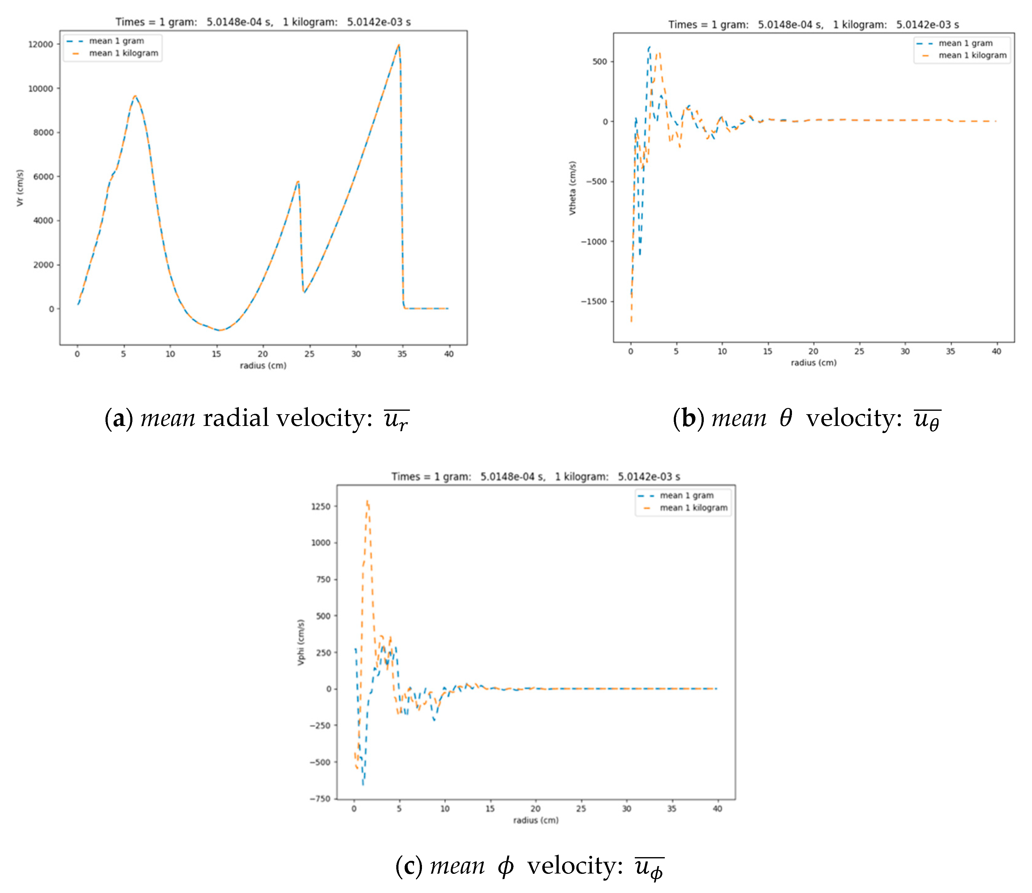
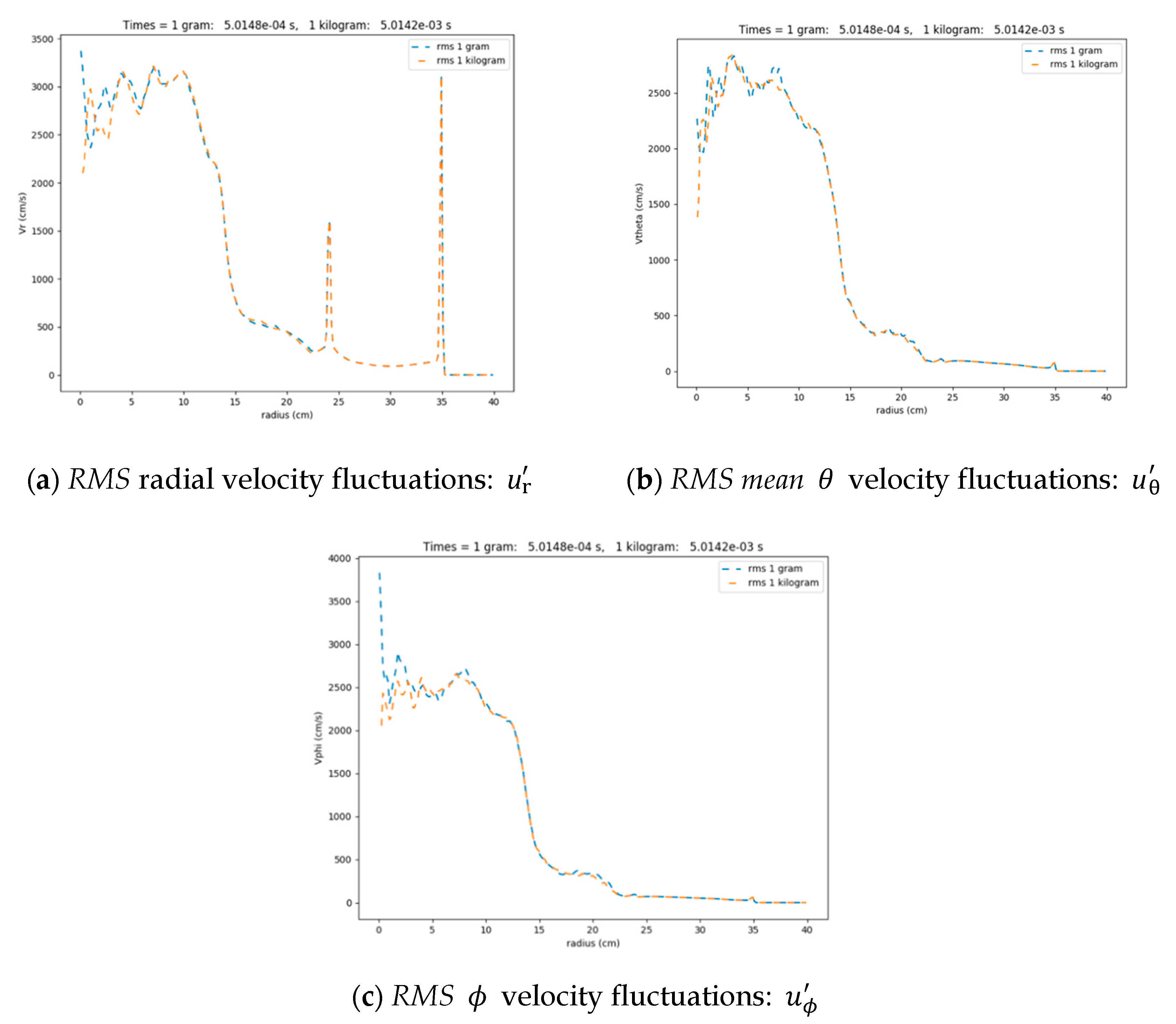
Figure 11 and Figure 12 depict azimuthally averaged velocity profiles () from a 1 g charge at (blue curves) compared with flow fields from the 1 kg charge at the same scaled time, (orange curves). The mean and RMS profiles from the two scales overlayed. Profiles of mean values for were essentially zero.
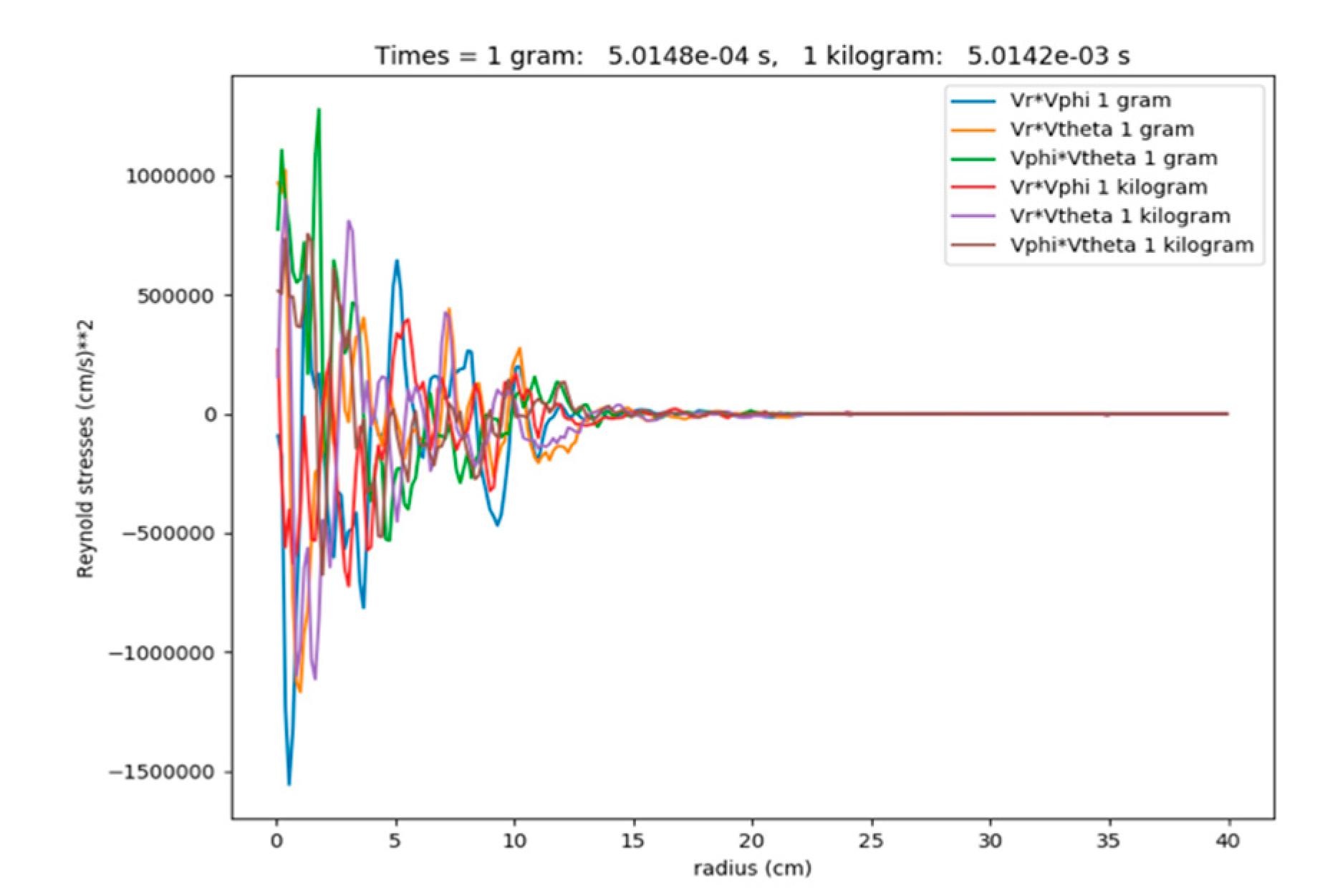
Figure 13 shows azimuthally averaged off-diagonal turbulent Reynolds stresses () from a 1 g charge at compared with flow fields from the 1 kg charge at the same scaled time, . The profiles were essentially zero, with random fluctuations due to the small ensemble size at small radii.
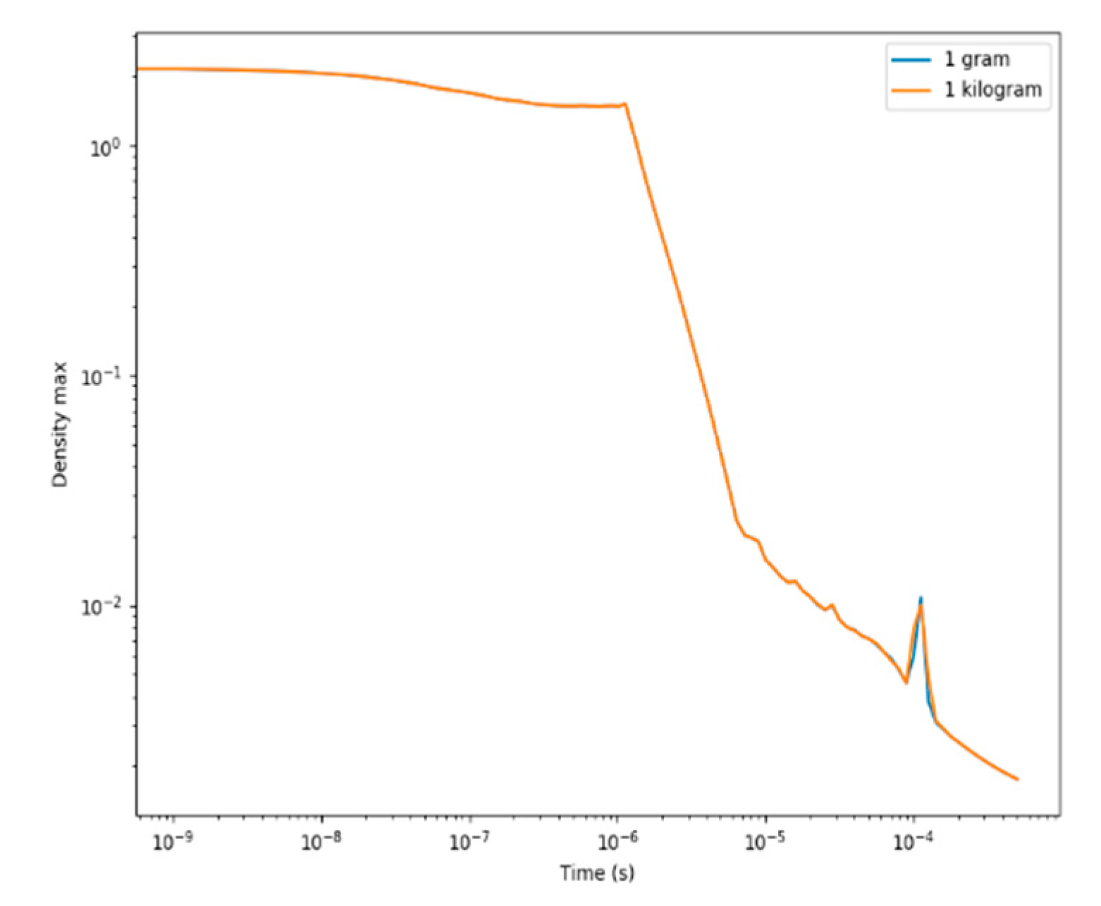
Figure 14 shows the maximum density histories for a 1 g charge (blue curve) and a 1 kg charge (orange curve); the curves overlayed. Maximum densities decayed because of the adiabatic expansion of the detonation products, with a spike at due to the imploding shock [20].
Figure 15 presents the combustion histories for 1 g and (blue curve) and scaled 1 kg charge (orange curve); the curves overlayed. About 50% of the fuel mass was consumed by combustion at this time.
Let us azimuthally average the fireball temperature field in to find the evolution of the mean temperature field with time:
Let us define the fireball radius as the radius where (starting from outside the fireball and working inward). Then, the evolution of the fireball radius becomes
Dividing by the initial nondimensional charge radius , one finds
From experiments and numerical simulations, when the spherical fireball has expanded to one atmosphere, one obtains
The largest characteristic scale in the turbulent fireball is the fireball radius, and thus turbules in the fireball scale with .
4.3. Summary
We confirmed the similarity of turbulent combustion fields of fireballs from HE explosions. Figure 16 presents turbulent fireball structures from our gadynamic simulations (Figure 16a,c), which are compared with a photograph of a fireball (Figure 16b). They show similar turbulent structures that scaled with the explosion length scale, .
As expected, all gasdynamic profiles (e.g., thermodynamic profiles, combustion profiles, velocity profiles, and Reynolds stresses), both their mean and RMS values, scaled with the explosion scale . The fireball radius scaled according to . To sum up, all aspects of gaseous turbulent combustion in HE explosions scaled with the explosion radius .
5. Three-Phase Pyrotechnic Explosions
Next, we considered pyrotechnic explosions. Figure 17 presents a cross-section of the three-phase temperature field of a pyrotechnic explosion from our paper in the 16th International Detonation Symposium [21]. It shows the turbulent mixing and combustion of the gas phase, which reached a temperature of 2500 (yellow regions) corresponding to the adiabatic flame temperature of the HE–air system. It also shows discrete Lagrange particles (black dots) that shed micro-mist wakes (red curves). This three-phase nature of such pyrotechnic explosions is what we explore in this section. Models are described next.
5.1. Gas Phase
The conservation laws of gas dynamics are used to model the expansion of the detonation products, mixing, and turbulent combustion of the detonation products with air. The gas phase is coupled to the particles and wakes phases with drag and heat transfer terms. The conservation laws of mass, momentum, total energy, and detonation products (DP) mass fraction are
where are the gas density, velocity, pressure, temperature, and mass-fraction of DP, respectively. Here, is the total energy and is the internal energy. The equation of state is specified by tables based upon the Cheetah code [11]. Drag and heat transfer effects with the particles and wakes are included in the source terms on the right-hand side of Equations (34) and (35).
5.2. Particle Phase
The dynamics of the particle phase is modeled by discrete Lagrange particles (DLPs) and their interactions with air, namely, mass, momentum, and energy [22]:
where denote the position, velocity, mass, and internal energy of particle i, and denotes gravity. Mass loss, drag, and heat transfer interactions with air are specified by the following relations:
where k represents thermal conductivity [k] = joules/(sec-m-K). The surface recession rate, , is based on measurements [23] and empirical modeling [24,25] of Al–air combustion systems. The following drag and Nusselt correlations [26] (Appendix C) are assumed:
5.3. Wake Phase
The wake phase is modeled by the heterogeneous continuum (HC) model of Nigmatulin [27] and Collins et al. [28]:
Drag and heat transfer interactions between wakes and gas are modeled by
The same drag and Nusselt correlations of Equations (44) and (45) are used.
5.4. Scaling of Pyrotechnic Explosions
The scaling laws for the gas phase were discussed in Section 2. For pyrotechnic explosions, we must deal with all three phases. One can say that the conservation laws for phases 2 and 3 describe inertial flow, since there are no pressure gradient forces. However, there are source/sink terms on the right-hand side of the equations, expressing mass transfer, drag, and heat transfer with the gas phase. They are functions of the Reynolds and Prandtl numbers. How these scale with change in problem scale is discussed below.
The initial conditions for a pyrotechnic charge are illustrated in Figure 2. It shows the detonation wave structure for the gas phase (as before) and the linear velocity profile for the droplet phase. This corresponds to similarity solution of inertial flow expansion into a vacuum, as published by Stanyukovich [15] in 1960. The ball radius of the droplet phase extends to 10% of the charge radius (i.e.,). These initial conditions scale with the explosion scale, , in other words . Thus, we consider two pyrotechnic explosion scales:
- •
- A full-scale charge (the dynamics of this pyrotechnic charge system was published in the 16th Detonation Symposium [21]) where with a mass of 7175 kg;
- •
- 1/3 scale charge where with a mass of 265.7 kg.
As mentioned above [21], the pyrotechnic charge contains a liquid ball of radius , and thus a full-scale charge would have a ball radius of , while a 1/3-scale charge would have a ball radius of . The ball is made up of droplets; we estimated the droplet diameter as , which will be the same for both scales. (We assumed the liquid sphere was put under strong radial strain, creating droplets. According to Tolman (1949) [29], the droplet size is controlled by surface tension, which is a material property. Thus, the droplet size will be the same for full scale and subscale.) The number of droplets scaled as , which was equal to 296,296 droplets at full scale and 10,974 at 1/3 scale. The droplet wake diameter scaled as , and thus was in both cases. The wake equilibration length scaled as , and thus the wake equilibration length was 30 cm in both cases. The droplet Reynolds number scaled as . Assuming a characteristic velocity of 1 km/s, one finds the droplet Reynolds number of , and the wake Reynolds number of . These have drag coefficients of and Nusselt numbers of (see Appendix C for more Nusselt number correlations versus data). These results are summarized in Table 1. We note that here the particle sizes introduced an additional length scale, and thus we did not expect to maintain self-similarity.
5.5. Gas Phase Results
We investigated the scaling behavior by comparing simulations at two different scales. Pyrotechnic fireball temperature cross-sections at 1/3 scale and full scale are presented in Figure 18. The azimuthally averaged pyrotechnic fireball temperature profiles are presented in Figure 19. Curves of the mean and RMS profiles are shown; profiles at 1/3 scale (blue curves) and full scale (orange curves) overlayed, i.e., they scaled with . It is interesting to note that the maximum mean fireball temperature in the pyrotechnic explosion was , which was lower than the HE fireball case of (see Figure 7a) because of heat losses to the DLPs.
5.6. DLP Phase Velocity Results
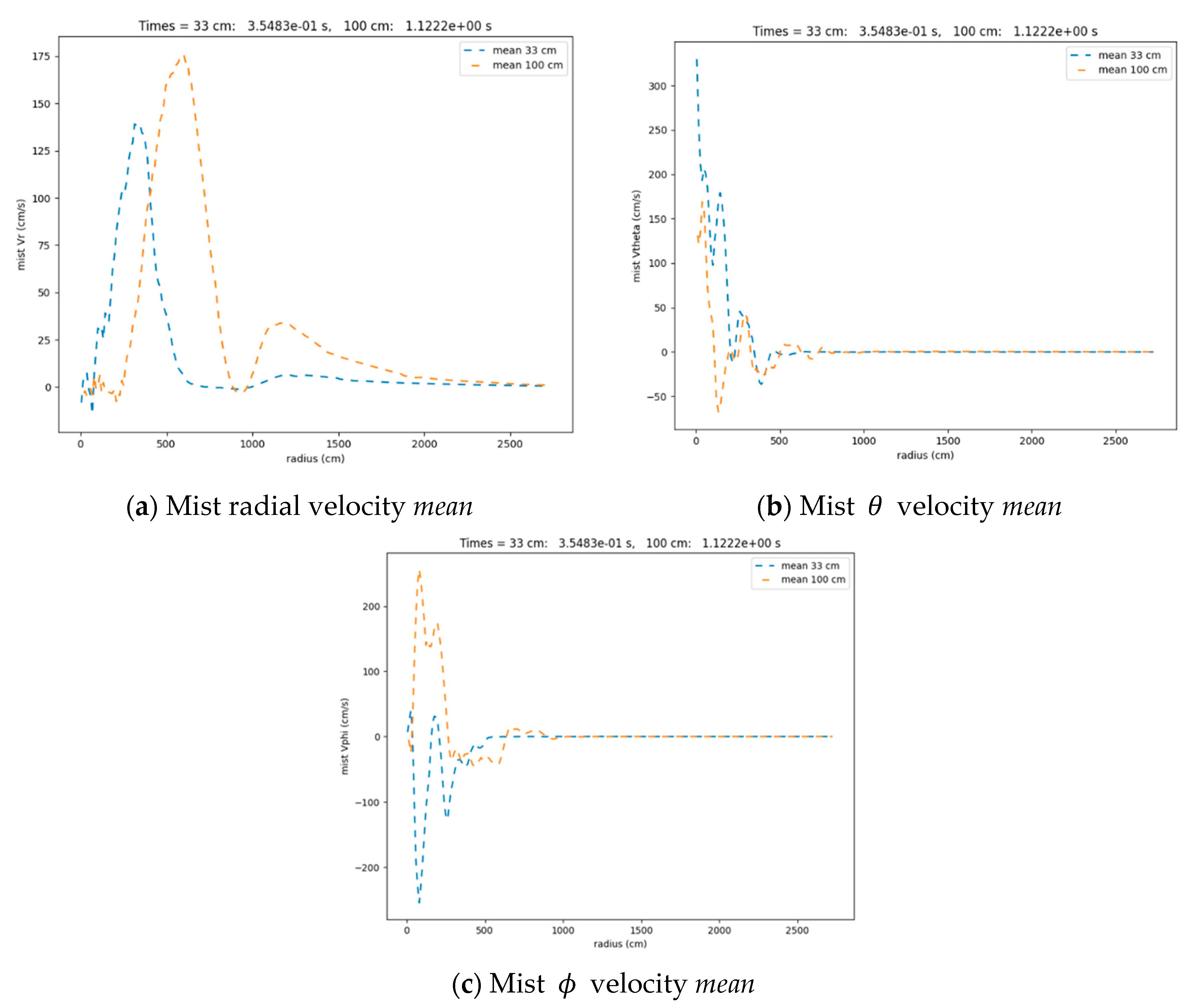
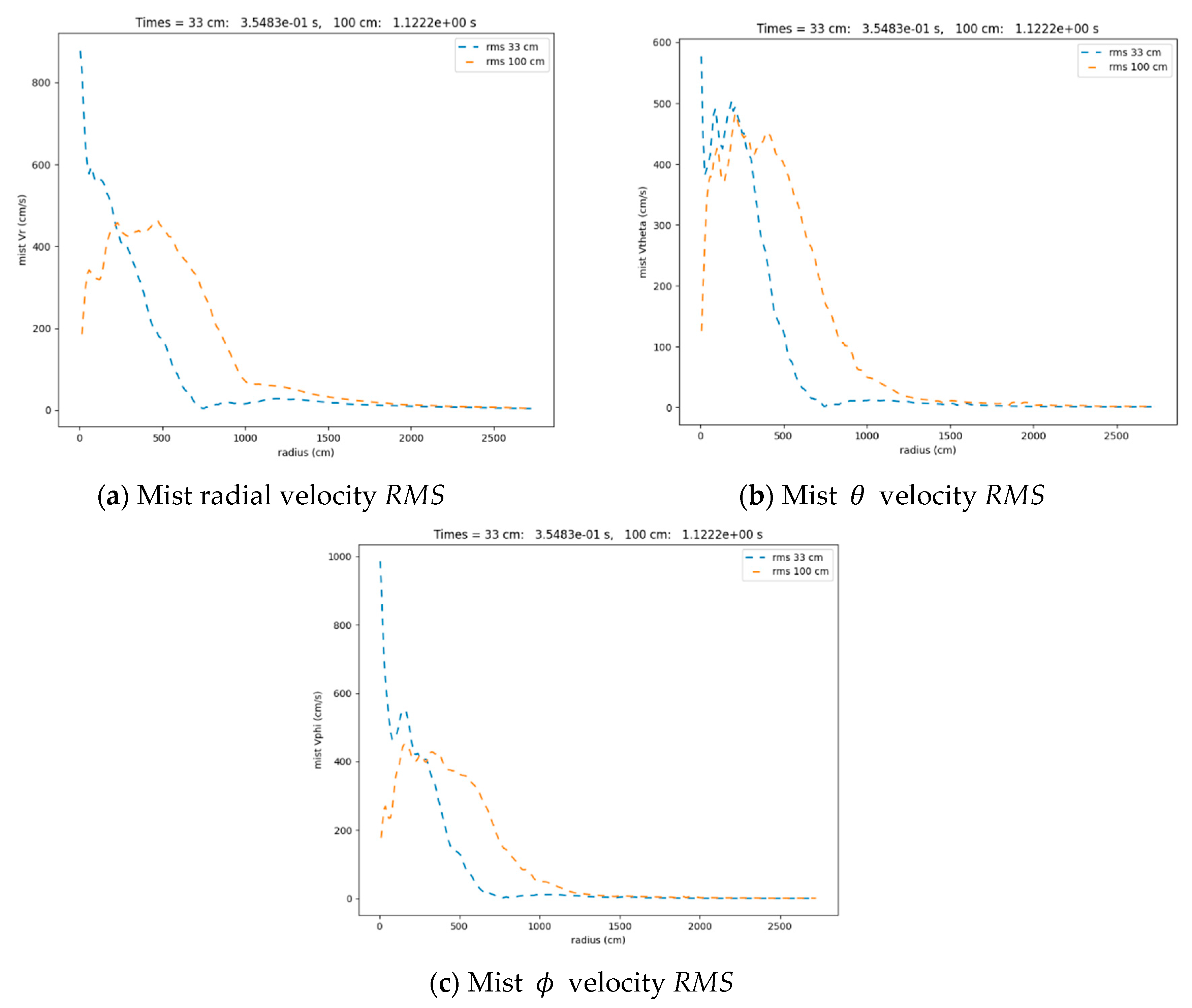
5.7. Mist Phase Results
Pyrotechnic fireball mist temperature cross-sections are presented in Figure 26. Their azimuthally averaged mean and RMS mist temperature profiles are shown in Figure 27. Results for 1/3 scale (blue curves) and full scale (orange curves) did not overlay, i.e., their profiles did not scale with .
5.8. Summary
A summary of the scaling laws for pyrotechnic explosions is given in Table 2. When implemented in the three-phase model (Equations (33)–(51)), one finds that
- •
- Turbulent combustion in the gas phase fireball does scale with ;
- •
- The DLP flow field does not scale with ;
The mist flow field does not scale with .
5.9. Conclusions
The gas phase of pyrotechnic explosions scaled with , indicating that the multi-phase effects did not disrupt the scaling behavior. The DLP particle phase behaved ballistically, being only subject to drag and heat transfer without pressure (blast wave) effects, and thus did not satisfy similarity conditions. The mist phase started with zero mass and was only created by a mass sink in the DLP equations. It also was inertial (i.e., devoid of pressure effects) and only subject to drag and heat transfer effects, and thus it also did not satisfy the similitude conditions.
6. Discussion
6.1. Initial HE Density Perturbations
When initializing the HE density profile shown in Figure 2, we introduced spatial sinusoidal variations with 1% maximum amplitude to break nonphysical numerical symmetries. This helped trigger the instabilities on the HE–air interface in order to make it less dependent on grid effects. To check whether these spatial perturbations might have any effect on scaling, we changed the sinusoidal base, and re-ran the HE fireball case shown in Figure 4, Figure 5, Figure 6, Figure 7, Figure 8, Figure 9, Figure 10, Figure 11, Figure 12, Figure 13, Figure 14 and Figure 15. The result was that the profiles of the two cases overlayed, and thus scaled with
6.2. Grid Refinement
We also explored the effect of grid refinement on scaling. We doubled the resolution and re-ran the HE fireball case shown in Figure 3, Figure 4, Figure 5, Figure 6, Figure 7, Figure 8, Figure 9, Figure 10, Figure 11, Figure 12, Figure 13, Figure 14 and Figure 15. Table 3 summarizes the profile comparisons of 1× versus 2× zoning. We found that a factor of 2 increase in grid resolution had no effect on the mean and RMS profiles of thermodynamic variables, , and mean velocity-related profiles of . The RMS profiles also scaled with , but had about 30% variation due to grid resolution.
7. Conclusions
We investigated scaling behavior for turbulent combustion fields in explosions. Sedov has derived a similarity theory for explosions, stating that the flow fields scale as and , where and . This theory was derived for the blast wave (dilatational) velocity field. However, according to the Helmholtz decomposition theorem [30,31,32], the velocity vector field can be divided into its dilatational and rotational components (see Appendix B). The dilatational component corresponds to the blast wave solution of Sedov. The rotational component corresponds to the turbulent velocity field found in the fireball of explosions. Our algorithm numerically satisfies the same scaling behavior discretely, and thus we expect the numerical solution for inviscid gaseous explosions to show the same scaling relation. The two solutions were identical when displayed in scaled variables (i.e., the flow field profiles only differed by machine roundoff).
Numerical simulations of pyrotechnic fireballs performed at two different scales confirmed this observation; their azimuthally averaged scaled profiles overlayed, proving that they scaled with . However, the DLP flow fields and the wake flow fields of pyrotechnic explosions did not scale with because particle sizes introduced another length scale that broke similarity. For example, scaled mist temperature, density, and velocity profiles can differ by a factor of 10 in certain regions. Thus, calculations and numerical simulations of pyrotechnic explosions must be performed at each scale of interest. This has not been recognized in the past.
Author Contributions
A.K. was responsible for the gas-dynamic formulation of the three-phase models used in this research; D.G. performed the numerical simulations reported here; J.B. led the development of the high-order Godunov algorithms and Adaptive Mesh Refinement methods used in the simulations reported here. All authors have read and agreed to the published version of the manuscript.
Funding
Lawrence Livermore National Laboratory is operated by Lawrence Livermore National Security, LLC, for the U.S. Department of Energy, National Nuclear Security Administration under Contract DE-AC52-07NA27344. This work was funded by the Office of Defense Nuclear Nonproliferation Research and Development.
Conflicts of Interest
The authors declare no conflict of interest.
Nomenclature
| Symbol | Definition |
| gas density | |
| gas velocity vector | |
| gas pressure | |
| gas total energy: | |
| gas internal energy | |
| mass fraction detonation products DP | |
| mass fraction of air | |
| mass fraction of fuel (detonation products) | |
| mass fraction of oxidizer (air) | |
| mass fraction of combustion products | |
| combustion rate | |
| stoichiometric air/fuel ratio | |
| vorticity vector | |
| baroclinic vorticity production: | |
| nondimensional radius: | |
| nondimensional time: | |
| explosion length scale: | |
| explosion time scale: | |
| mass of the high explosives charge | |
| heat of detonation | |
| geometry index j = 0, 1 or 2 for planar, cylindrical, or spherically symmetric flow | |
| R | nondimensional density function: |
| nondimensional velocity function: | |
| nondimensional internal energy function: | |
| nondimensional pressure function: | |
| nondimensional temperature function: | |
| nondimensional dilatational velocity: | |
| nondimensional rotational velocity: | |
| nondimensional Cartesian coordinates: , , | |
| fireball radius | |
| high explosives charge radius | |
| liquid ball radius | |
| high explosives charge mass | |
| number of i droplets: | |
| number of droplets i per unit volume: | |
| droplet i equilibration length | |
| mean | azimuthally averaged mean value |
| RMS | azimuthally averaged root mean squared value |
| dilatational velocity | |
| rotational velocity | |
| drag force | |
| heat transfer | |
| number of particles per unit volume | |
| position of particle i | |
| velocity of particle i | |
| mass of particle i | |
| surface recession rate of particle i | |
| specific internal energy of particle i | |
| diameter of particle i | |
| drag coefficient | |
| Nusselt coefficient | |
| Reynolds number | |
| Prandtl number | |
| thermal conductivity | |
| density of the wake phase | |
| velocity of the wake phase | |
| energy of the wake phase | |
| number of wake particles per unit volume: | |
| mass of the wake phase in cell: | |
| mass of air in cell | |
| mass of fuel in cell | |
| Subscripts | |
| 0 | characteristic scale |
| a | ambient conditions |
| FB | fireball |
| c | charge |
| i | particle i |
| D | drag |
| w | wake |
| B | ball |
| r | radial velocity |
| theta velocity | |
| phi velocity | |
| Chapman–Jouguet state | |
Appendix A. Azimuthal Averaging
We took advantage of the spherical symmetry of the problem and azimuthally averaged the flow fields. We transformed Cartesian coordinates to spherical coordinates: . Consider a spherical shell volume at radius :
Let us say that the shell thickness is equal to the cell size, . Points within a shell are denoted by , while flow field variables within a shell are denoted by . Then, one can define a mean flow field variable by
Given the mean , one can then define the fluctuation by
Then the root mean squared (rms) fluctuation becomes
The accuracy of the azimuthally averaged variables depends on the ensemble size, N. The number of points in the ensemble is shown in Table A1.

Table A1.
Ensemble size, N.
| 1 | 2000 |
| 5 | 0.5 × 10⁵ |
| 10 | 2 × 10⁵ |
| 15 | 4.6 × 10⁵ |
| 20 | 8 × 10⁵ |
for .
For radii outside of 5 cm, one has 105 samples, which gives a good average. For radii inside 5 cm, there may not be enough points to give an accurate average.
Appendix B. Helmholtz Velocity Decomposition
The complete velocity field is computed by the second order Godunov scheme [16,17]. According to Equation (25), both the dilatational and rotational velocity components scale according to
In particular, the above points out that the rotational velocity component —i.e., the turbulent velocity field—also scales with the explosion length scale, .
Under suitable asymptotic behavior at infinity, an arbitrary velocity vector field can be decomposed into two parts: a dilatational component , which is irrotational, plus a rotational component, , which is solenoidal:
where
with and denoting scalar and vector potentials, respectively. They satisfy the following Poisson equations:
and
Appendix C. Nusselt Number Correlation for Turbulent Flow
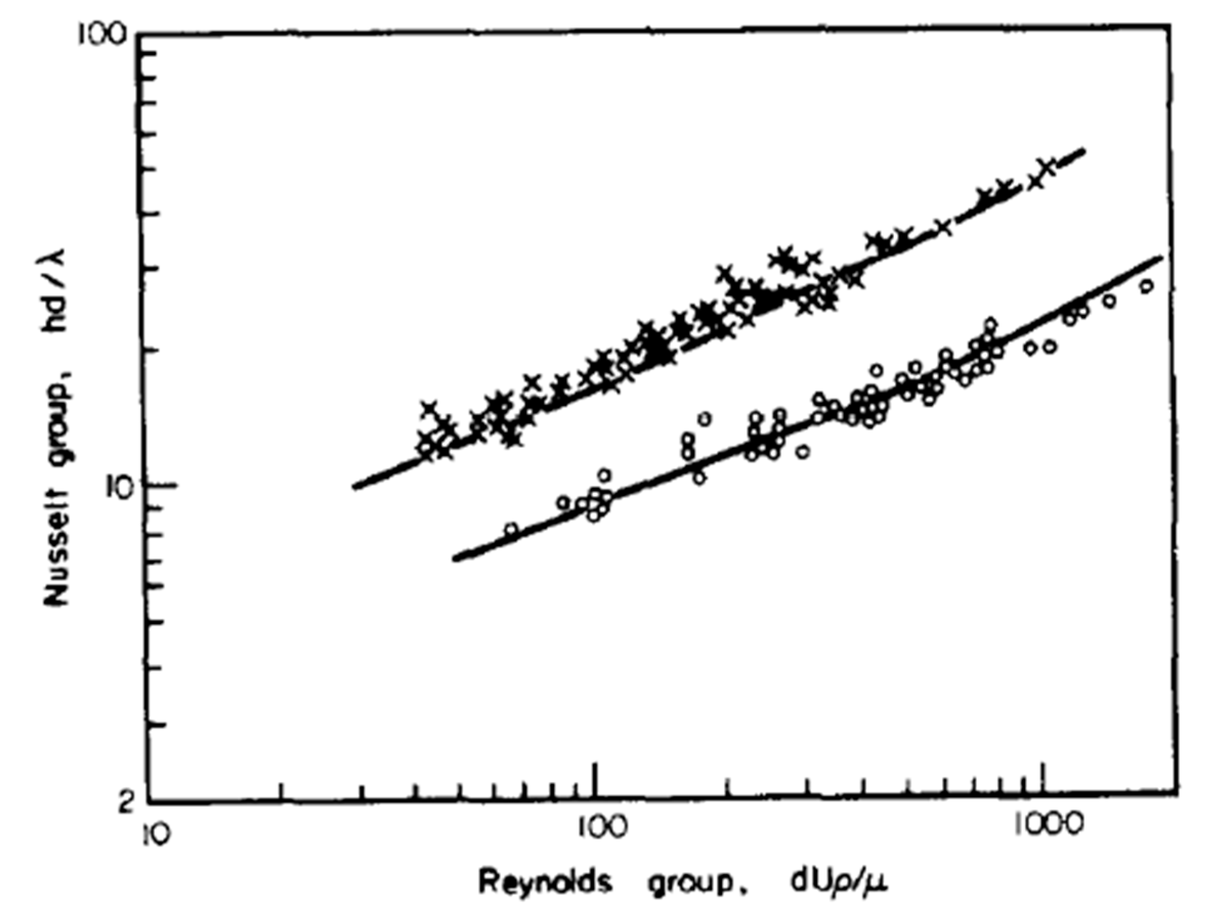
Gunn [22] has correlated the nondimensional heat transfer coefficient of a sphere, the Nusselt number, with experimental data for water and air. Results are shown in Figure A1. The data are correlated with the following function:
where e denotes the bed voidage, Re represents the Reynolds number, and Pr is the Prandtl number. For a voidage of 1, this reduces to the following:
Figure A1.
Experimental results of Rowe, Claxton, and Lewis for heat transfer to a single sphere comparted with full lines calculated from equation (C1); X water, O air.
Figure A1.
Experimental results of Rowe, Claxton, and Lewis for heat transfer to a single sphere comparted with full lines calculated from equation (C1); X water, O air.

References
- Bridgman, P.W. Dimensional Analysis; Yale University Press: New Haven, CT, USA, 1922; p. 40. [Google Scholar]
- Buckingham, E. On physically similar systems; illustrations of the use of dimensional equations. Phys. Rev. 1914, 4, 345. [Google Scholar] [CrossRef]
- Sedov, L.I. Similarity and Dimensional Methods in Mechanics; Academic Press: New York, NY, USA, 1959. [Google Scholar]
- Taylor, G.I. The formation of a blast wave by a very intense explosion. Br. Rep. RC-210 1941, 201, 175–186, later published in Proc. R. Soc. A 1950, 201, 175–186. [Google Scholar]
- Sedov, L.I. Propagation of strong blast waves. Prikl. Mat. Mech. 1946, 10, 241–250. [Google Scholar]
- Oppenheim, A.K.; Kuhl, A.L.; Lundstrom, E.A.; Kamel, M.M. A parametric study of self-similar blast waves. J. Fluid Mech. 1972, 52, 657–682. [Google Scholar] [CrossRef]
- Oppenheim, A.K.; Kuhl, A.L.; Kamel, M.M. On self-similar blast waves headed by the Chapman-Jouguet detonation. J. Fluid Mech. 1972, 55, 257–270. [Google Scholar] [CrossRef]
- Barenblatt, G.I.; Guirguis, R.H.; Kamel, M.M.; Kuhl, A.L.; Oppenheim, A.K.; Zel’dovich, Y.B. Self-similar explosion waves of variable energy at the front. J. Fluid Mech. 1980, 99, 841–858. [Google Scholar] [CrossRef]
- Barenblatt, G.I. Scaling, Self-Similarity, and Intermediate Asymptotics; Cambridge University Press: Cambridge, UK, 1996; p. 190. [Google Scholar]
- Glumac, N.; Kuhl, A.L. Optical emissions from spherical charges. In Proceedings of the 21st Biennial Conference APS Topical Group on Shock Compression of Condensed Matter (SHOCK19), Portland, OR, USA, 16–21 June 2019. [Google Scholar]
- Fried, L.E. CHEETAH 1.22 User’s Manual, UCRL-MA-117541; Lawrence Livermore National Laboratory: Livermore, CA, USA, 1995. [Google Scholar]
- Bastea, S.; Fried, L.E. Chemical Equilibrium Detonation. In Shock Wave Science and Technology Reference Library; Zhang, F., Ed.; Springer: Berlin/Heidelberg, Germany, 2012; Volume 6, p. 1. [Google Scholar]
- Boris, J.P. On large eddy simulation using sub-grid turbulence models-Comment 1, Wither turbulence? In Turbulence at the Crossroads; Lecture Notes in Physics; Lumley, J.L., Ed.; Springer: Berlin/Heidelberg, Germany, 1989; Volume 257, pp. 344–353. [Google Scholar]
- Kuhl, A.L. On the structure of self-similar detonation waves in TNT charges. Combust. Explos. Shock. Waves 2015, 51, 72–79. [Google Scholar] [CrossRef]
- Stanyukovich, K.P. Unsteady Motion of Continuous Media; Pergamon Press: London, UK, 1960; 749p, (see especially § 63. Expansion of Gaseous Sphere in a Vacuum, pp. 498–501 & Equation 63:13). [Google Scholar]
- Colella, P.; Woodward, P. The Piecewise Parabolic Method (PPM) for gas-dynamical simulations. J. Comp. Phys. 1984, 54, 174–201. [Google Scholar] [CrossRef] [Green Version]
- Miller, G.H.; Colella, P. A Conservative Three-Dimensional Eulerian Method for Coupled Solid-Fluid Shock Capturing. J. Comp. Phys. 2002, 183, 26–82. [Google Scholar] [CrossRef] [Green Version]
- Berger, M.J.; Colella, P. Local adaptive mesh refinement for shock hydrodynamics. J. Comp. Phys. 1989, 82, 64–84. [Google Scholar] [CrossRef] [Green Version]
- Bell, J.B.; Berger, M.; Saltzman, A.; Welcome, M. Three-dimensional Adaptive Mesh Refinement (AMR) for hyperbolic conservation laws. SIAM J. Sci. Stat. Comput. 1994, 15, 127–138. [Google Scholar] [CrossRef]
- Brode, H.L. Blast wave from a spherical charge. Phys. Fluids 1959, 2, 217–229. [Google Scholar] [CrossRef]
- Kuhl, A.L.; Grote, D.; Almgren, A.; Bell, J.B. Hydrodynamics of pyrotechnic explosions. In Sixteenth International Detonation Symposium; 22217-5660, ORNL-43-5762-19; Office of Naval Research: Arlington, VA, USA, 2018; pp. 1203–1212. [Google Scholar]
- Kuhl, A.K.; Grote, D. Modeling Expansion of Particle Clouds. LLNL-TR-718339. 2017. Available online: http://www.icders.org/ICDERS2017/abstracts/ICDERS2017-0986.pdf (accessed on 26 November 2020).
- Ingignoli, W. Étude de la Formation et de la Propagation des Détonations dans des Suspensions de particules D’aluminium en Atmosphère Oxydante ou Réactive. Ph.D Thesis, d’Université de Poitiers, Poitiers, France, 1999; 495p. [Google Scholar]
- Khasainov, B.; Kuhl, A.L.; Victorov, S.; Neuwald, P. Model of non-premixed combustion of Al–air mixtures. AIP Conf. Proc. 2005, 845, 449–452. [Google Scholar]
- Kuhl, A.L.; Bell, J.B.; Beckner, V.E. Heterogeneous continuum model of Aluminum particle combustion in explosions. Combust. Explos. Shock. Waves 2010, 46, 433–448. [Google Scholar] [CrossRef]
- Gunn, D.J. Transfer of heat or mass to particles in fixed and fluidized beds. Int. J. Heat Mass Transf. 1978, 21, 467–476, {see Equation (4.1) for e = 1: }. [Google Scholar] [CrossRef]
- Nigmatulin, R.I. Dynamics of Multi-Phase Flows; Nauka: Moscow, Russia, 1987; Volume 1. [Google Scholar]
- Collins, J.P.; Ferguson, R.E.; Chien, K.-Y.; Kuhl, A.L.; Krispin, J.; Glaz, H. Simulation of shock-induced dusty gas flows using various models. In Proceedings of the AIAA Fluid Dynamics Conference 94-2309, Colorado Springs, CO, USA, 20–23 June 1994. [Google Scholar]
- Tolman, R. The effect of droplet size on surface tension. J. Chem. Phys. 1949, 17, 333–337. [Google Scholar] [CrossRef] [Green Version]
- Batchelor, G.K. An Introduction to Fluid Dynamics; Cambridge University Press: Cambridge, UK, 1967; pp. 84–87. [Google Scholar]
- Morino, I. Helmholtz decomposition revisited: Vorticity generation and trailing edge condition. Comput. Mech. 1986, 1, 65–90, {vid. esp. Equation (2.12)}. [Google Scholar] [CrossRef]
- Hodge, W.V.D. The Theory and Applications of Harmonic Integrals; Cambridge Press: Cambridge, UK, 1941. [Google Scholar]
Figure 1.
Fireball image from a 15-kg COMP B spherical charge at 4 m height of burst.

Figure 2.
Initial conditions based on the similarity solutions for a Chapman–Jouguet (CJ) detonation wave in the gas phase by Kuhl [14], and the linear velocity profile of an inertial flow expansion into a vacuum by Stanyukovich [15] for the droplet phase.

Figure 3.
Exothermic flame sheet in the TNT–air combustion field at .

Figure 4.
Comparison of the cross-section of the density fields.

Figure 5.
Comparison of the cross-section of the vorticity fields.

Figure 6.
Maximum density difference between the 1 g case and the 1 kg case as a function of time. Differences stayed at roundoff errors until , when they grew exponentially at late times.
Figure 6.
Maximum density difference between the 1 g case and the 1 kg case as a function of time. Differences stayed at roundoff errors until , when they grew exponentially at late times.

Figure 7.
Comparison of the mean thermodynamic profiles at (1 g charge) and (1 kg charge).


Figure 8.
Comparison of the RMS thermodynamic profiles at (1 g charge) and (1 kg charge).

Figure 9.
Comparison of the mean combustion component profiles at (1 g charge) and (1 kg charge).

Figure 10.
Comparison of the RMS combustion component profiles at (1 g charge) and (1 kg charge).


Figure 11.
Comparison of the mean velocity profiles at (1 g charge) and (1 kg charge).

Figure 12.
Comparison of the RMS velocity profiles at (1 g charge) and (1 kg charge).

Figure 13.
Off-diagonal turbulent Reynolds stresses were essentially zero.

Figure 14.
Maximum density histories for 1 g and 1 kg charges.

Figure 15.
Combustion histories of fuel and products for 1 g and 1 kg charges.

Figure 16.
Turbulent fireball structures from simulations (a,c) are compared with an experimental photograph in frame (b) from Glumac and Kuhl [10].
Figure 16.
Turbulent fireball structures from simulations (a,c) are compared with an experimental photograph in frame (b) from Glumac and Kuhl [10].

Figure 17.
Cross-section of a pyrotechnic explosion predicted by our three-phase code [21].
Figure 17.
Cross-section of a pyrotechnic explosion predicted by our three-phase code [21].

Figure 18.
Pyrotechnic fireball temperature cross-section at early times.

Figure 19.
Azimuthally averaged pyrotechnic fireball temperature profiles.

Figure 20.
Pyrotechnic fireball vorticity cross-sections.

Figure 21.
Azimuthally averaged fireball vorticity profiles for pyrotechnic explosion.

Figure 22.
Azimuthally averaged mean combustion profiles for pyrotechnic explosions.

Figure 23.
Azimuthally averaged RMS combustion fluctuation profiles for pyrotechnic explosions.

Figure 24.
Azimuthally averaged mean discrete Lagrange particle (DLP) velocity profiles for pyrotechnic explosions.
Figure 24.
Azimuthally averaged mean discrete Lagrange particle (DLP) velocity profiles for pyrotechnic explosions.


Figure 25.
Azimuthally averaged RMS DLP velocity profiles for pyrotechnic explosions.

Figure 26.
Fireball mist temperature cross-sections for pyrotechnic explosions.

Figure 27.
Azimuthally averaged mist temperature profiles for pyrotechnic explosions.

Figure 28.
Fireball mist density cross-sections for pyrotechnic explosions.

Figure 29.
Azimuthally averaged mist density profiles for pyrotechnic explosions.

Figure 30.
Azimuthally averaged mean mist velocity profiles for pyrotechnic explosions.

Figure 31.
Azimuthally averaged RMS mist velocity fluctuation profiles for pyrotechnic explosions.

Table 1.
Comparison of radii, drag, and heat transfer for pyrotechnic droplet explosions (di = 3 mm).
Table 1.
Comparison of radii, drag, and heat transfer for pyrotechnic droplet explosions (di = 3 mm).
| Variable | Scaling | Scale = 1 | Scale = 1/3 |
|---|---|---|---|
| ———Initial Conditions——— | |||
| HE charge radius | 100 cm | 100/3 cm | |
| HE charge mass (Comp B) | kg | kg | |
| Liquid ball radius; diameter | 10 cm; 20 cm | 10/3; 20/3 cm | |
| Droplet diameter | 3 mm | 3 mm | |
| Number of droplets | |||
| Droplets per unit volume | 37/cc | 37/cc | |
| Droplet equilibration length, | 30 m | m | |
| Droplet wake diameter, | |||
| Wake equilibration length, | |||
| ——— Drag & Heat Transfer Effects ——— | |||
| Droplet Reynolds number * | |||
| Droplet drag coefficient | 0.481 | 0.481 | |
| Droplet Nusselt number [23] | 40 | 40 | |
| Wake Reynolds number | |||
| Wake drag coefficient | 0.48 | 0.48 | |
| Wake Nusselt number [23] | 40 | 40 | |
* characteristic velocity u = 1 km/s is assumed.
Table 2.
Scaling summary.
| Variable | Scaled |
|---|---|
| HE charge radius, | |
| Ball radius, | |
| Droplet diameter, * | |
| Wake mist diameter, | |
| Number droplets, | |
| Droplets per unit volume, | |
| Droplet Reynolds number, | |
| Wake Reynolds number, |
* is controlled by surface tension; this value is estimated from experiments.
Table 3.
Summary of grid resolution on mean and RMS profiles.
| Variable | mean | RMS |
|---|---|---|
| OK * | OK | |
| OK | OK | |
| OK | -- | |
| ~ OK ) | ~ OK ( | |
| OK | OK | |
| OK | OK | |
| OK | ~ OK ( | |
| OK | ~ OK ( |
* OK scales with , .
Publisher’s Note: MDPI stays neutral with regard to jurisdictional claims in published maps and institutional affiliations. |
© 2020 by the authors. Licensee MDPI, Basel, Switzerland. This article is an open access article distributed under the terms and conditions of the Creative Commons Attribution (CC BY) license (http://creativecommons.org/licenses/by/4.0/).
Share and Cite
MDPI and ACS Style
Kuhl, A.; Grote, D.; Bell, J. Scaling Turbulent Combustion Fields in Explosions. Appl. Sci. 2020, 10, 8577. https://doi.org/10.3390/app10238577
AMA Style
Kuhl A, Grote D, Bell J. Scaling Turbulent Combustion Fields in Explosions. Applied Sciences. 2020; 10(23):8577. https://doi.org/10.3390/app10238577
Chicago/Turabian StyleKuhl, Allen, David Grote, and John Bell. 2020. "Scaling Turbulent Combustion Fields in Explosions" Applied Sciences 10, no. 23: 8577. https://doi.org/10.3390/app10238577
Note that from the first issue of 2016, this journal uses article numbers instead of page numbers. See further details here.