
Determination of Hygroscopic Aerosol Growth Based on the OPC-N3 Counter

Institute of Geophysics, Faculty of Physics, University of Warsaw, 00-927 Warsaw, Poland
*
Author to whom correspondence should be addressed.
Atmosphere 2024, 15(1), 61; https://doi.org/10.3390/atmos15010061
Submission received: 14 November 2023
/
Revised: 12 December 2023
/
Accepted: 23 December 2023
/
Published: 31 December 2023
(This article belongs to the Special Issue Aerosol Pollution in Central Europe)
Abstract
:We present the first estimations of single hygroscopic parameter for Polish urban area. The results were obtained using an inexpensive OPC-N3 optical particulate matter counter and the ASC 1000 Acoem Aerosol Conditioning System. Our studies were carried out during the winter and spring seasons, between 2020 and 2022 in Warsaw, Poland. We study the difference of between these two seasons, as the aerosol has different origins. The mean value of the hygroscopicity parameter for spring (April–June) was and for winter (December-March) it was (obtained using PM). The mean value of the growth factor for spring (April–June) was and for winter (December–March) it was (obtained using PM). The values for winter period suggest that during the cold season the aerosol mixture in the atmosphere is dominated by non-hygroscopic particles. However events of higher > 0.5 where occurring (mostly for big aerosol particles 1–10 m in size), when the air mass was coming from North Atlantic carrying sea salt particles. Furthermore, based on we propose a method to remove the dependence of PM values on relative humidity on the OPC-N3 optical particulate counter.
1. Introduction
Aerosol particles directly and indirectly affect the Earth’s climate. The Intergovernmental Panel on Climate Change (IPCC) [1] assigned a great uncertainty to this influence. Aerosols scatters and absorb radiation, some act as the onset of cloud condensation nuclei furthermore they interacts with cloud droplets. The hygroscopicity is a key factor which influences those processes.
Particulate matter is one of the wildly monitored atmospheric compounds in the world. The high mass concentration of PM in the atmosphere can be associated with health problems [2,3]. For this reason several countries introduced limits of concentration for PM diameter lower than 2.5 m (PM) and 10 m (PM) [4,5]. The amount of PM changes rapidly in time and space. Polish cities are often exposed to values above the norm [6]. The concentration of PM can be different in distinct parts of the city (the reason for this may be the amount of traffic, the way of heating houses, and land use). For this reason, more dense measurement networks are created. To lower the cost of such systems, the low-cost apparatus is needed. The low-cost optical particle counters, like OPC-N3, can elevate the PM values in high RH. This can cause alerts of poor air conditions despite the fact that the actual level of PM is normal. For such reasons PM counters should operate with dehumidifiers or should be corrected on the RH of surrounding air. The OPC-N3 measures PM, PM and PM. The measured PM values significantly relay on the air’s relative humidity.
When relative humidity (RH) is high, aerosols in the air have reservoir of water, therefore can grow larger and scatter more light. Parameters such as refractive index, angular scattering, size, or shape are sensitive to dousing aerosol particles with water. Typically, to remove the effects induced by hygroscopic growth the optical properties of the aerosol such as the scattering coefficient are obtained in low relative humidity (RH < 40%) [7]. The hygroscopicity of an aerosol can be characterized in several different ways, e.g., by the change of radius between wet and dry particles, by the mass ratio of wet and dry particles, or by the change of the light scattering coefficient between wet and dry particles. To assess the size of the hygroscopic effect one can calculate an enhancement factor, where the scattering coefficient in a given RH is divided by the scattering coefficient in dry conditions. Most scattering coefficient measurements are carried out in low RH conditions; however, for the proper operation of climate models, it is necessary to know the changes occurring when water begins to condense on aerosols. In fact, in the Arctic the enhancement effects is pronounced due to the presence of more sea salt in the air. Zieger et al. [8] demonstrate that the mean scattering enhancement factor in this region is 3.2.
Assuming incorrect values of growth factors in models can lead to biasing of the results. Zieger et al. [9] shows that the hygroscopicity of sea salt is different from the hygroscopicity of sodium chloride (many works assumed the hygroscopicity is the same). Furthermore correcting the parameter which describe the hygroscopicity in a global climate model provide differences in aerosol optical depth (AOD) in some areas by almost [9].
The Köhler theory describes how the particle will grow exposed to a certain RH level. To calculate the activity of cloud condensation nuclei (CCN) based on this theory, one needs to know the solute mass, dissociable ions, and other physicochemical properties. Petters and Kreidenweis [10] proposed a single dimensionless parameter to describe the hygroscopicity. Introduction of this parameter allowed to assign one parameter to a mixture of different aerosols or assigning a single value to molecules consisting of insoluble core immersed in aqueous solution.
Petters and Kreidenweis [10] calculated the values of for atmospheric aerosols. For typical aerosols found in the atmosphere values lie between . The = 0 denotes substances non-hygroscopic, while a highly higroscopic aerosol is often found in the marine atmosphere (sodium chloride reaches the value = ). The article by Petters and Kreidenweis [10] neglected soot, which can be found in polluted urban areas. The values of for soot range between 0 and [11]. The calculation of is possible by fitting nonlinear curve with one parameter to the relation between growth factor and air RH.
Aerosol present in the atmosphere is a mixture of particles with different chemical composition. In this case, one parameter is used to describe the resulting hygroscopicity of the mixture of different particles. The chemical compound of the aerosol is also crucial to describe its behavior under various RH conditions. Under the influence of high RH, some particles may be covered with water (adsorption) or dissolve in water (absorption), causing further changes in their properties [12].
Aerosols display various behaviors on the basis of their interaction with environmental conditions. Some aerosols remain insoluble in water and maintain a relatively stable size even when exposed to higher RH levels, such as soot. Others, such as sulfuric acid (HSO), are soluble and undergo diameter changes when exposed to varying levels of RH. There are also aerosols that expand as humidity increases, yet they have specific markers in a humidogram known as the deliquescence point (DRH) and efflorescence point (ERH).
DRH and ERH represent critical junctures in the humidogram where the solid core of the aerosol dissolves or crystallizes, triggering sudden alterations in particle size [13]. It’s important to note that DRH and ERH are distinct points, emphasizing the significance of an aerosol’s history in determining its growth factor at a given RH [14].
The hygroscopic growth of the aerosol may have a significant impact on its undesirable effects on the human respiratory tract. Inhaling aerosols can deeply penetrate the respiratory system, impacting lung function and potentially aggravating respiratory conditions. Notably, in Poland, comprehensive studies regarding the hygroscopic properties of aerosols have not been conducted, creating a gap in understanding their behavior in the atmosphere. Aerosols’ hygroscopic nature significantly influences their behavior, altering their size, composition, and ability to act as cloud condensation nuclei. Moreover, the optical properties of aerosols undergo considerable modifications when exposed to varying RH levels. These changes in optical properties play a vital role in visibility, atmospheric radiative budget, and climate dynamics. Therefore, investigating aerosol hygroscopicity becomes critical for assessing health risks and understanding the broader atmospheric and climatic implications. Addressing this research gap within the context of Poland is crucial for accurately modeling climate changes induced by aerosol-humidity interactions.
The article has the following structure in Section 2 are presented instruments and in Section 3 digital tools used in data acquisition and analysis. Section 4 focus was on utilizing OPC-N3 alongside ACS 1000 (Aerosol Conditioning System) to gauge the hygroscopic nature of urban aerosols. The data were gathered from the and GF measurements taken at the Radiation Transfer Laboratory (RTL) site between 2020 and 2022. Given the absence of prior studies on aerosol hygroscopicity in Poland, our aim was to identify typical values. Additionally, in Section 4.3 we sought to uncover instances of heightened hygroscopicity and their underlying causes, which led us to present two case analyses. The Section 5 introduces a method for adjusting OPC-N3 PM values based on the surrounding RH. The latter part (Section 6) summarised the obtained results. Finally, Section 7 comprises the conclusions drawn from the results.
2. Instruments
2.1. OPC-N3
The OPC-N3 is a small (105 g) low-cost optical particle counter developed by Alphasense Ltd. It is composed of a diode laser of 658 nm wavelength and an elliptical mirror that reflects light to a photodiode detector. The flow is perpendicular to the laser beam and a fan is used to maintain a continuous flow. The device can measure the particle number concentration (PNC) in 24 bins, ranging from 0.35 to 40 m diameter. The PNC is then converted to PM, PM and PM. As shown by Nurowska et al. [15], OPC-N3 is capable of registering water droplets, in addition to registering aerosols.
As stated in [16], previous studies report that Alphasense OPCs demonstrate strong correlations (R2 = 0.93–0.99) with PM10 in controlled laboratory investigations [17,18,19,20]. However, field-based studies have indicated relatively lower correlations (R2: 0.53–0.8) [21,22,23], primarily due to the variability in ambient meteorological conditions and fluctuations in PM compositions. More information on Alphasense OPC-N3 can be found in [24].
2.2. ACS 1000
Acoem (previously known as Ecotech) Aerosol Conditioning System ACS 1000 (Aerosol Conditioning System) is an indoor instrument capable of measuring the hygroscopic properties of aerosol particles. The ariflow is from the top to the bottom of the aparatus; at the top, air enters a tube where it is dehumidified (RH ) and then divided into two separate flows. At the end of two tubes, in which the air can be subjected to various conditions, there are outlets for connecting an external apparatus to carry out air measurements. One flow passes through a humidifier tube in which RH can be changed in a range from RH above ambient relative humidity (minimum RH ) up to (we refer to this tube as wet channel). The second flow, without any additional conditions, is directed to the connected measuring instruments. The flow rate can be adjusted in the range from 1 to 10 L·min. The ACS 1000 can change RH constantly or pass through some points in cycles. One cycle is set as a continuous change in relative humidity from the minimum level RH to the maximum level RH, then returns to the minimum relative humidity level RH. To perform faster cycles the return from maximum to minimum RH was abrupt, therefore the data collected only during the changing of RH from low to high were used for later analysis.
2.3. LAS
The Laser Aerosol Spectrometer (LAS) model 3340, manufactured by TSI, is a device that is used to measure the size distribution of atmospheric aerosol particles in the range from 90 to 7500 nm. It is capable of measuring 100 particle size classes. The measurements were conducted in a 5-min time resolution. This instrument is connected to the air intake system in the Radiation Transfer Laboratory (22 m a.g.l.).
2.4. GIOŚ
Polish Chief Inspectorate of Environmental Protection (GIOŚ) has air quality measurement station at Ave. Niepodległości, Warsaw (52.22 N 21.00 E) located 1.74 km from RTL. The air inlet of the station is approximately 5 m a.g.l. This is an automatic station measuring: benzene, carbon monoxide, nitrogen monoxide, nitrogen dioxide, nitrogen oxides, PM, PM with time resolution one hour (data is available to download [25]).
2.5. MERRA-2
The Modern-Era Retrospective analysis for Research and Applications, Version 2 (MERRA-2) [26] is a long-term global reanalysis from NASA Global Modelling and Assimilation Office, which assimilates space-based observations of aerosols. It has a resolution of 0.5° lat × 0.625° lon × 72 pressure levels. In this paper, we used the 3D aer_NV collection. The data were interpolated for the point of location of the measurements. We extracted the data about the aerosol mass mixing ratios from the lowest model layer (72: The vertical layers of MERRA-2 are arranged top-down). Concentrations of PM and PM have been calculated using Equations (1) and (2) [27]:
2.6. HYSPLIT
HYSPLIT (Hybrid Single-Particle Lagrangian Integrated Trajectory) is a model developed in 1998 by the National Oceanic and Atmospheric Administration (NOAA) and the Australian Bureau of Meteorology Research Centere. HYSPLIT is capable of computation of air parcel trajectories. In this article it was used to calculate the back trajectories of air parcels that flowed over Warsaw. We calculated the origin of air parcels 24 and 48 h before arriving at the Radiation Transfer Laboratory, Warsaw. The calculations were done for 00:00UTC and 12:00UTC for altitude 500 m using meteo data GDAS.
3. Methods
3.1. Data Acquisition
The experiment was carried out at the Institute of Geophysics of the University of Warsaw. The building is located in an urban area, location 52°12′40.7″ N 20°58′58.8″ E. The RTL is situated on the roof of the Faculty of Physics, where measurements of the optical and microphysical characteristics of atmospheric aerosols and clouds are constantly taken (e.g., with LAS 3340), as well as components of radiation fluxes and sensible and latent heat fluxes at the Earth’s surface. The basic atmospheric parameters are collected by the Vaisala WXT 520 weather station. The platform is located 20 m above the ground.
The inlet for the sampled air was located on the roof of the building (22 m a.g.l) and connected to the ACS 1000. At the inlet, air was drained (RH ) and then divided into two routes. In the wet pipe, the RH was changed in cycles (the RH was changed from around 55 to 90% and back to 55%—we refer to such a run as one cycle). In the other tube, the airflow was not modified (dry channel). At the outlets of the wet and dry channels, two identical devices were connected-OPC-N3.
The data analyzed come from the period between 2020 and 2022. The data were not assembled continuously (during autumn measurements at another location were performed). Data were collected in months between December and June; Table 2 presents the respective measurement times.
3.2. Data Calibration
By manual ACS 1000 should be able to operate in the range of RH between RH ( above ambient RH) up to . During winter, it was possible to obtain an average minimum RH below and for spring (The obtained minimum RH for each cycle was with standard deviation ± 4%). We were always trying to reach the minimum possible RH in the cycle.
The OPC-N3s were calibrated to each other seven times (listed in Table 2), approximately every new month of measurements. The calibration of both OPC-N3 was performed for RH below the threshold listed in Table 2.
Data from OPC-N3 were reported every 10 s and ACS 1000 every 6 s. In the first step, the PM, PM and PM from OPC-N3 were interpolated with the data from ACS 1000. Second, both OPC-N3 sensors were calibrated to each other by the least squares fit, the fitting coefficients are listed in Table A1. To denoise the data, a running average of 12 points was used.
3.3. -Köhler Theory
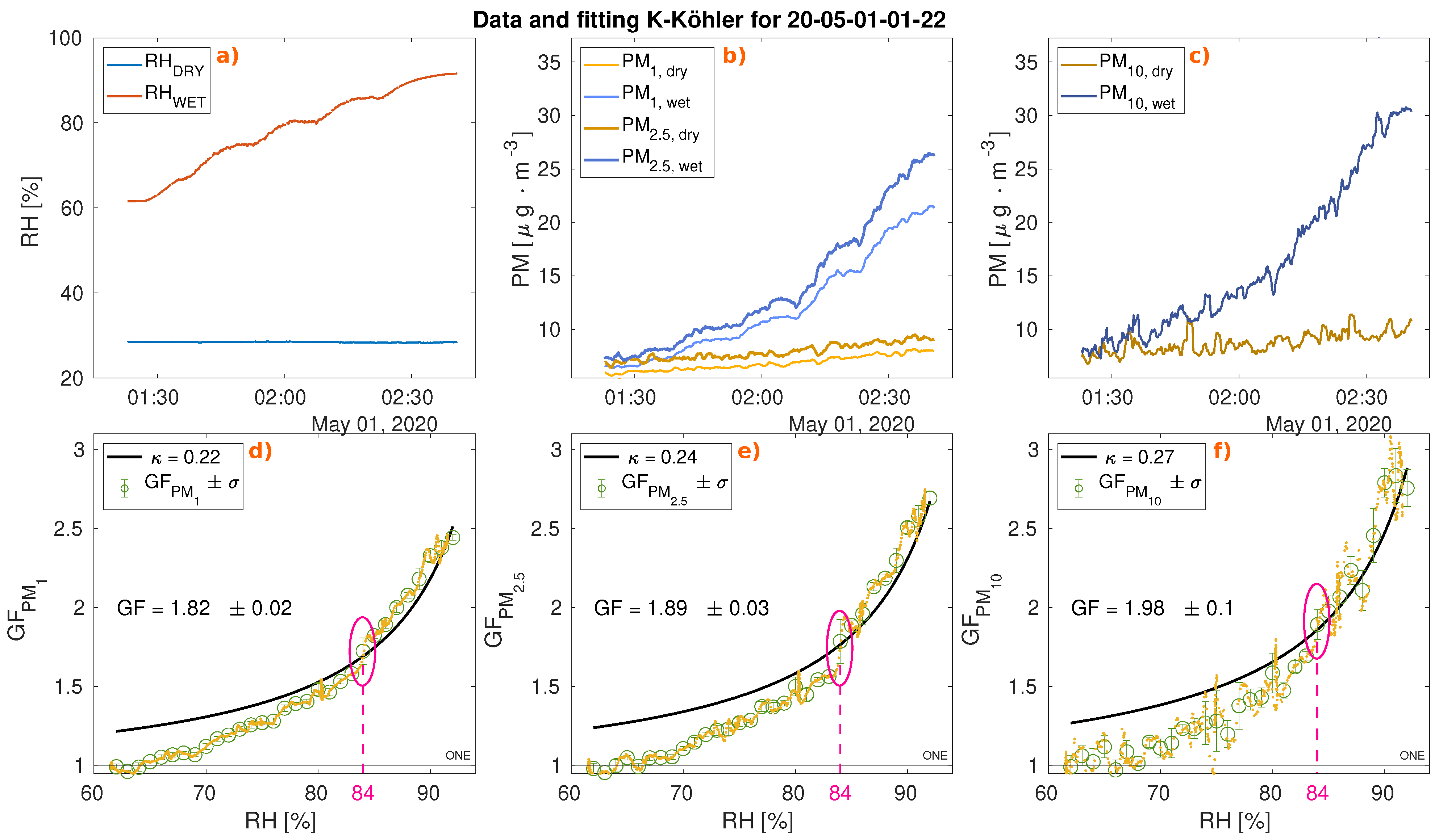
To obtain information about hygroscopicity of atmosphere aerosol the parameter proposed by Crilley et al. [21] was calculated. This parameter was obtained for each cycle performed by ACS100. As stated above (Section 2) the data collected during changing of RH from low to high were used for analysis. Figure 1d show one cycle of ACS100 with the RH from dry/wet brunch, Figure 1e,f show the PM, PM and PM respectively from both brunches.
The growth factor (GF) is defined by the equation:
where PM denotes particulate matter and denotes conditions in which RH is high and indicates some reference level in which RH is low (RH ).
Crilley et al. [21] proposed a formula to determine the dimensionless hygroscopicity coefficient .
where GF is an aerosol growth factor, RH denotes relative humidity, —water density 1.0 [g·cm] and —internal aerosol density parameter set in OPC-N3 sensors at 1.65 [g·cm]. The developed curve for describe the relation of hygroscopic growth of particle and RH above the deliquescent point. Extending the fit to lower RH values overestimates the hygroscopic growth of the aerosol (see Figure 1), the same effect was observed by Crilley et al. [21]. In Figure 1a,b, the deliquescence point (DRH) is visible, when the core of the aerosol particle dissolves in the water that pours over the body of the particle.
The was calculated for each cycle. Figure 1a–c shows obtained for one cycle from PM, PM and PM data respectively. The non-linear fit of Formula (4) was performed on the GF data as a function of RH. The Levenberg-Marquardt non-linear least squares algorithm was used [29]. Sometimes the fitted was below 0. For cases that was between −0.05 and 0, the value of was changed to 0 (This refers to a case when particles were not hygroscopic and did not grow in high RH). If fitted was lower than such cases were excluded from further analysis.
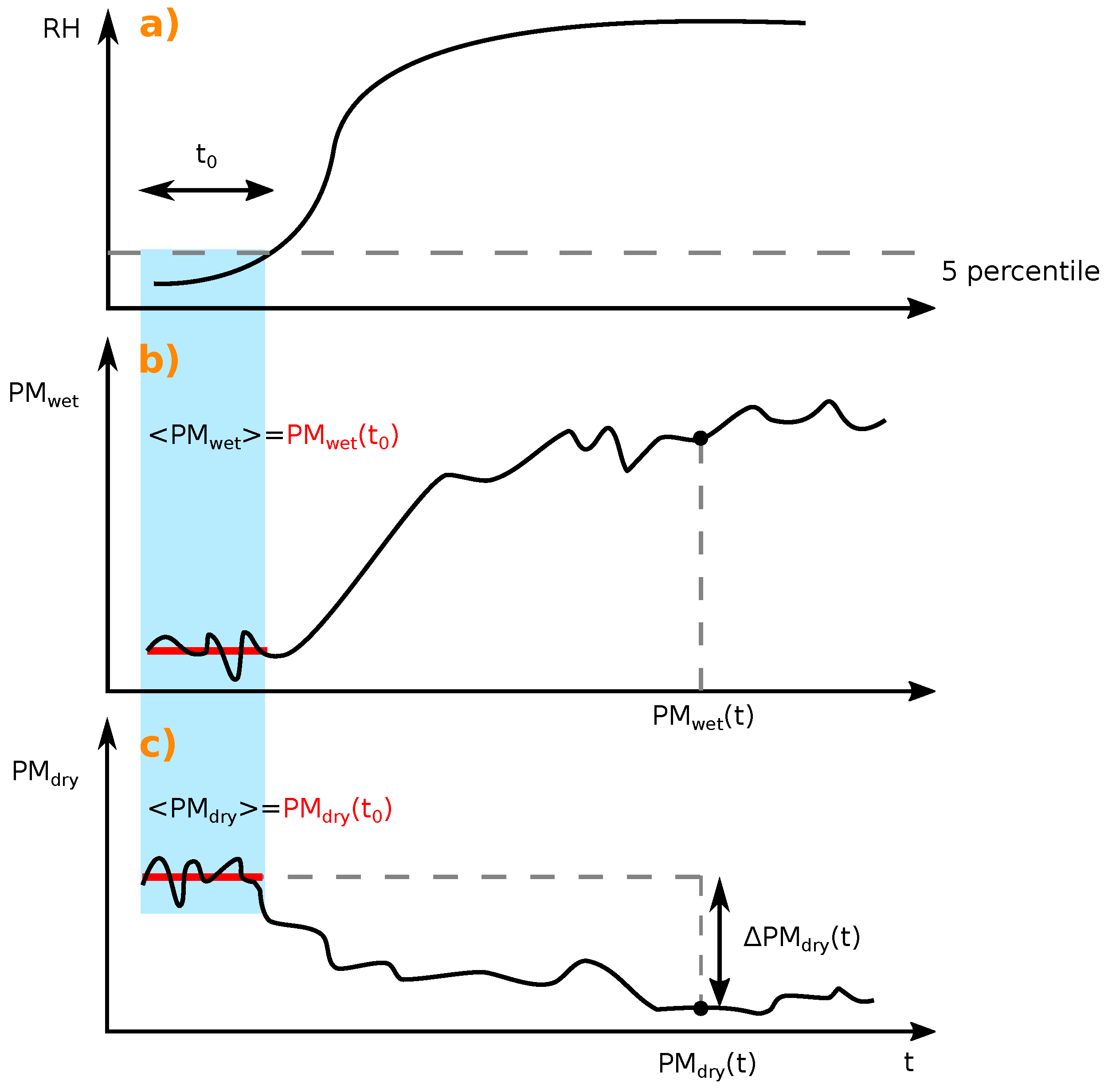
To calculate the GF, the following method was used for each cycle (graphically illustrated in Figure 2). The data from the wet brunch were used to calculate the GF. For each cycle, the average value of PM was calculated at time (), defined as a moment when the RH in the wet chamber was up to 5 percentiles.
As during the cycle, the external conditions could change, data from dry brunch were used to correct data at the wet brunch. It was determined what is the change in PM between a given moment and . The difference thus determined was added to the PM at a given time point. The data in the next step was divided by the mean PM value at the time .
4. Results
4.1. Half Year Variability
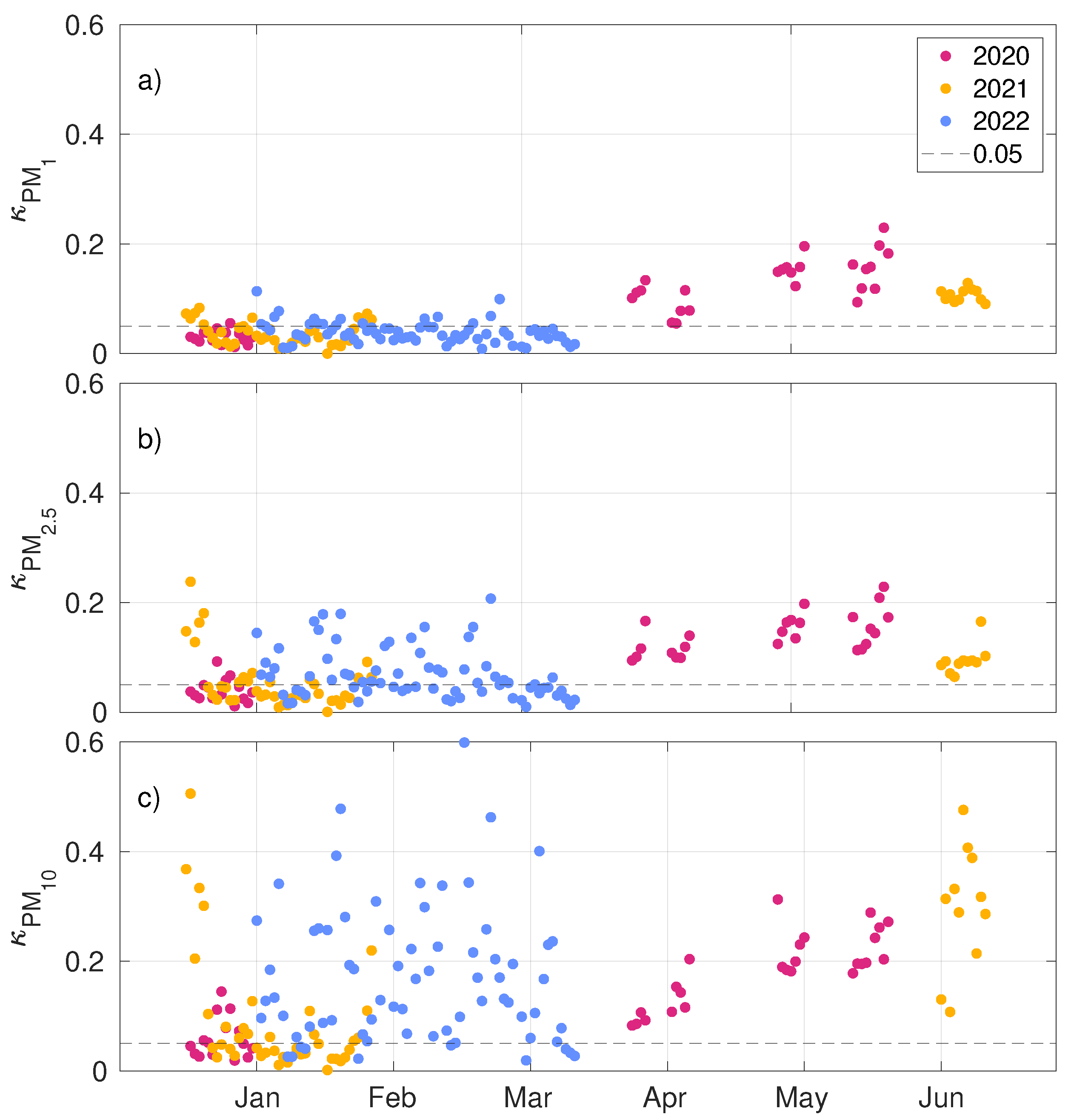
During one day several cycles were performed, therefore to show half year variability the data were averaged for each day. The Figure 3 show the calculation of parameter for three consecutive years (2020–2022) for months December–June, each panel corresponds to calculation of from a different particle matter size: panel (a) PM, panel (b) PM, panel (c) PM.
In the figure it is possible to observe that during the months December-March (later refereed as winter) ( obtained from PM data) is mostly below 0.05. However, more variation is visible for , ( obtained, respectively, from PM, PM data). For winter period only mixture of large particles (above 1 m) is subject to hygroscopic growth, and mixture of particles which diameter is smaller than 1 m is consisting mostly of non hygroscopic aerosols ( below 0.1).
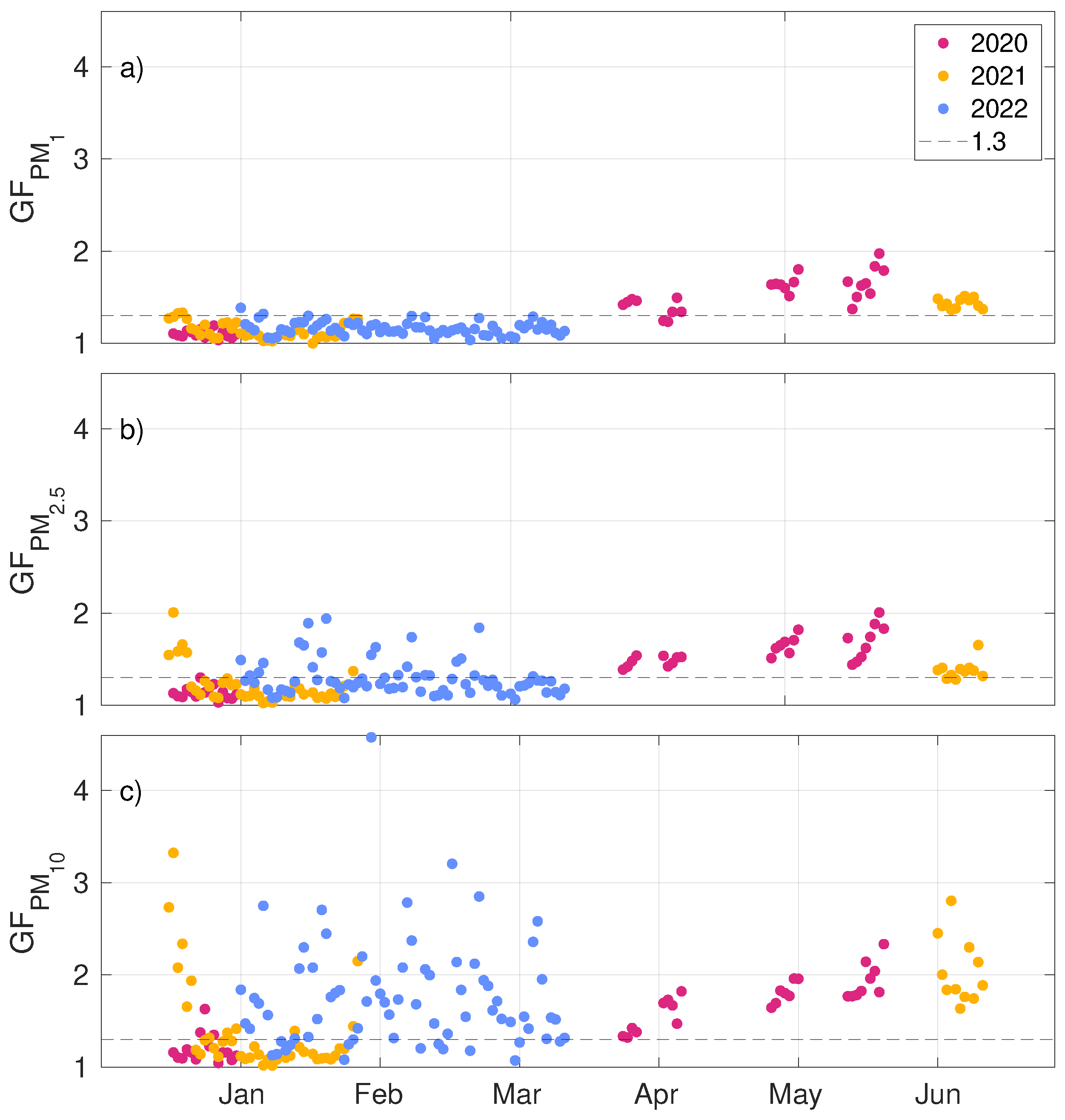
The same behavior can be seen if instead of parameter is calculated GF (see Figure 4). There is a very high Pearson correlation coefficient between GF and calculated from the same PM sizes. The correlation coefficient between vs. GF is 0.98, vs. GF is 0.97 and vs. GF is 0.89. All possible correlation coefficients between GF and kappa for different particle sizes are presented in Table 3. There is a high correlation coefficient between GF vs. GF (0.78) and vs. (0.77) and medium correlation coefficient between GF vs. GF (0.63), vs. (0.62). Correlations of GF and obtained from PM shows a weak correlation with respect to GF and obtained from PM. Due to the low concentration of particles of several micrometers in size, the PM data show significant Poisson noise. The lower correlation may also be due to the different chemical composition of small and large particles, which is why they are subject to different hygroscopic growth processes.
During winter varied from 0 to 0.11 (mean value ), 0 to 0.24 () and 0 to 0.60 (mean value ). During the spring varied from 0.05 to 0.23 (mean value ), 0.06 to 0.23 (mean value ) and 0.11 to 0.48 (mean value ). During the winter GF varied from 1 to 1.48 (mean value ), GF 1.02 to 2.00 () and GF 1.02 to 4.58 (mean value ). During the spring GF varied from 1.24 to 1.97 (mean value ), GF 1.28 to 2.00 (mean value ) and GF 1.32 to 2.80 (mean value ). The /GF and /GF for winter were mostly below 0.05/1.3 and for spring mostly above 0.05/1.3.
4.2. Diurnal Variation
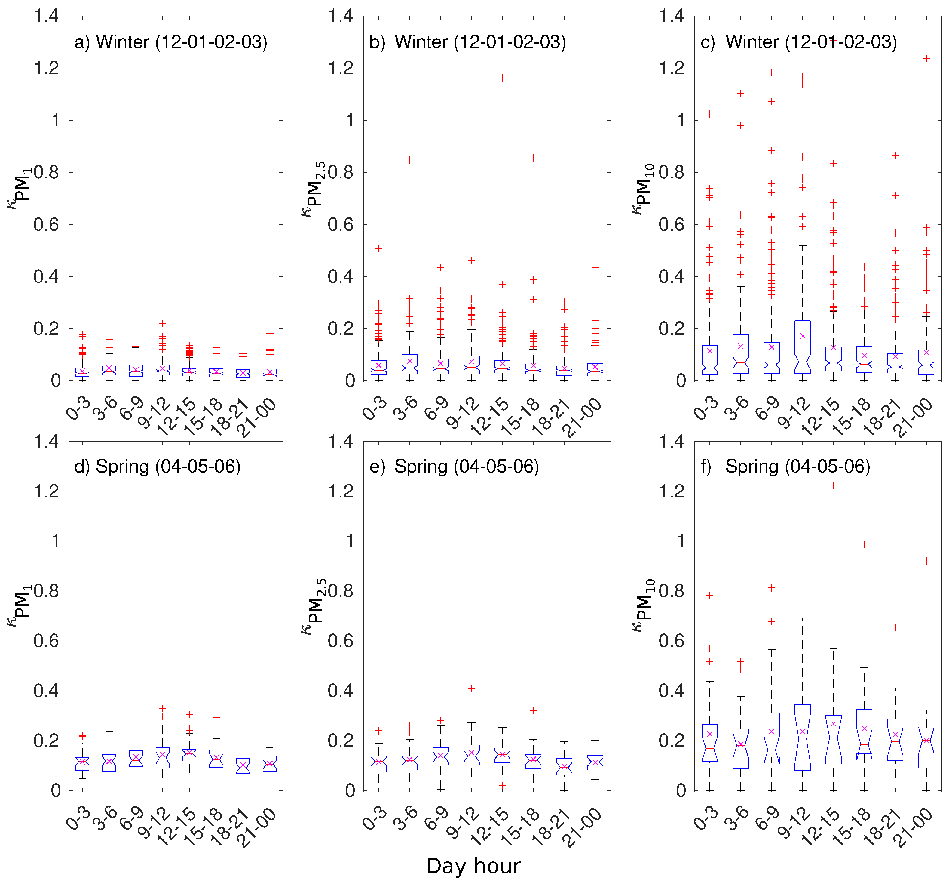
We were curious if the higroscopicity depends on diurnal variation. The Figure 5 presents the diurnal variation of parameter. Periods of winter and spring were depicted separately as the air aerosol composition differ between those seasons. For winter we found out (using one-way analysis of variance ANOVA) a statistically-significant difference in , and according to time of day (F(statistical F-test)(7) = 5.1, F(7) = 3.15, F(7) = 3.02, p < 0.05). A Tukey’s honestly significant difference criterion (TukeyHSD) revealed significant pairwise differences during winter season Table 4:
- for between time slot 18–21 and 3–6, 6–9, 9–12, with a difference of above 0.01 (p < 0.05),
- for between time slot 3–6 and 15–18, 18–21, 21–00, 00–03, with a difference of above 0.01 (p < 0.05),
- for between time slot 18–21 and 3–6, 9–12, with an average difference of 0.03 (p < 0.05),
- for between time slot 9–12 and 15–18, 18–21, with an average difference of 0.07 (p < 0.05).
For spring we found out a statistically-significant difference in , according to time of day (F(7) = 3.51, F(7) = 2.91, p < 0.05). A TukeyHSD revealed significant pairwise differences:
- for between time slot 12–15 and 18–21, 21–00, with an average difference of 0.05 (p < 0.05),
- for between time slot 18–21 and 9–12, 12–15 with an average difference of 0.05 (p < 0.05),
For during spring period no statistically-significant difference was found.
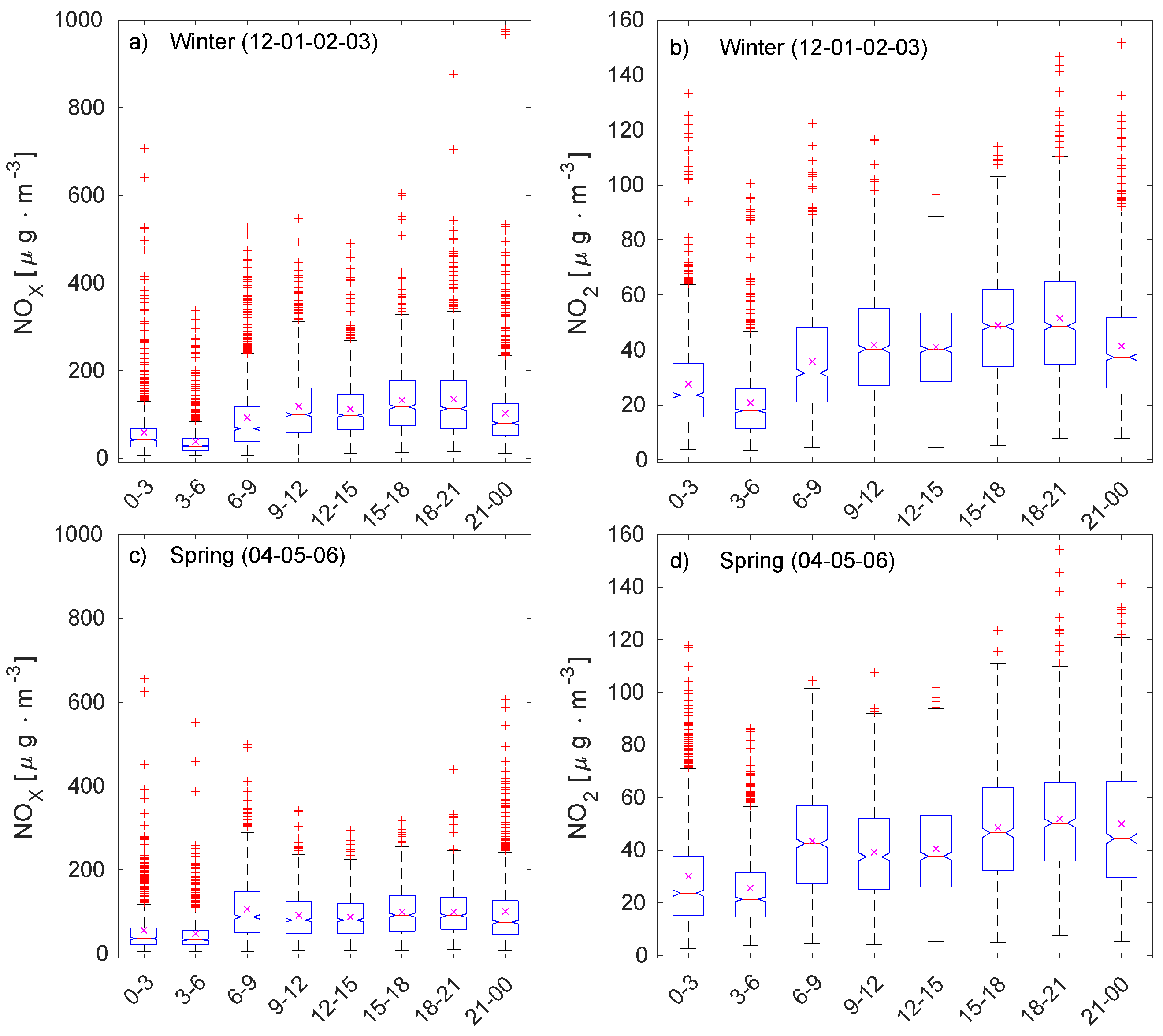
For winter, there is a significant difference in mean between the 9–12 and 18–21 time slot; and during spring, between the 12–15 and 18–00 time slots. Elevated values of during sun operating hours may be related to the production of photocemical particulate matter. As shown for the Los Angeles area by Dale A. Lundgren [30], during dense photochemically produced smog, particulate matter was mainly a water-soluble nitrate compound, which was very hygroscopic. In the Figure A1 we present the diurnal variation of NO and NO with regard to time of a day. The correlation between mean daily concentration of NO/NO and is not statistically significant, although it is slightly positive for spring and negative for winter. Based on this, it’s difficult to determine a direct link between aerosol hygroscopicity and public transportation emission.
4.3. Case Study
4.3.1. Winter 2021/2022 (15 December 2021–31 January 2022)
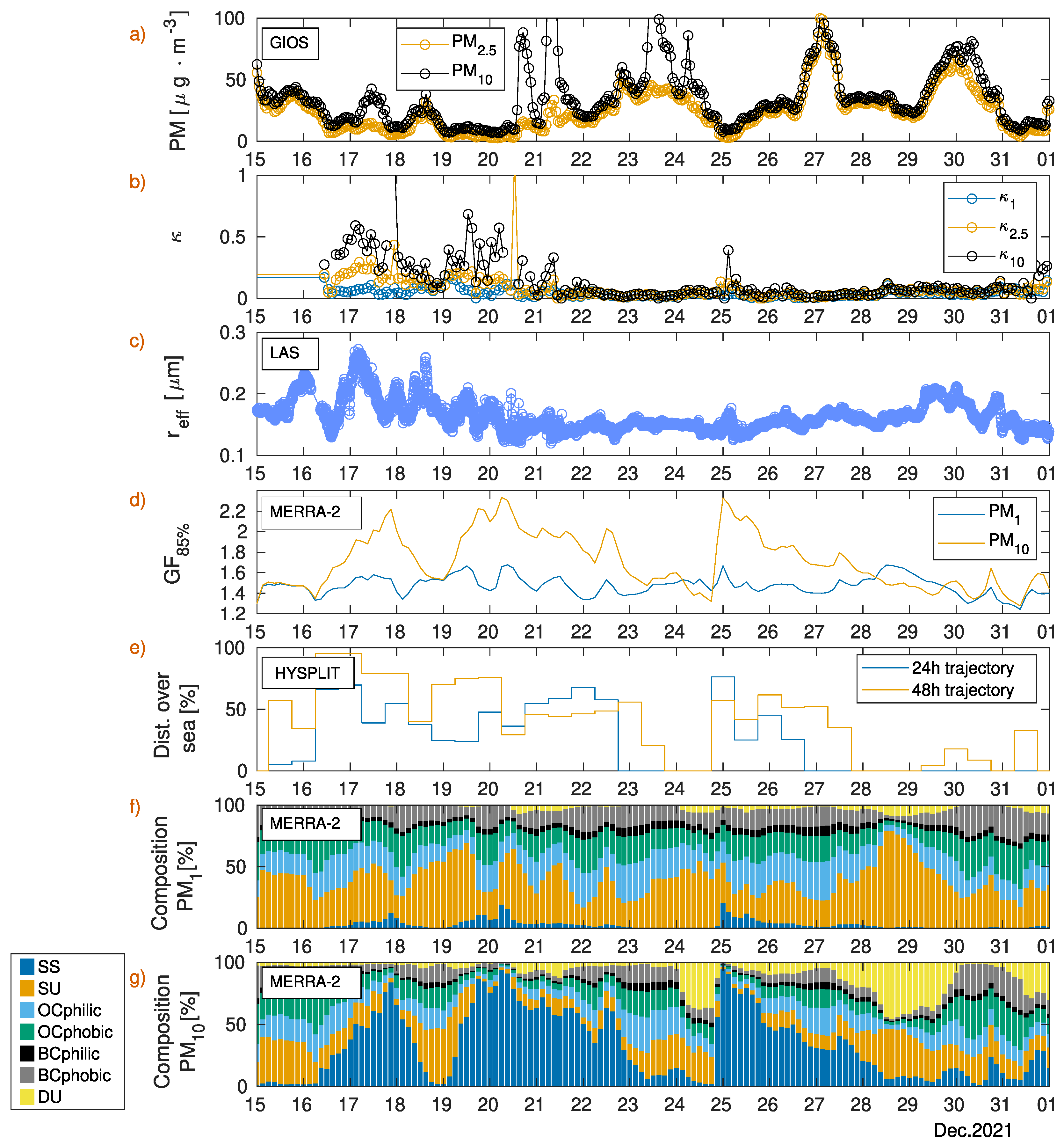
To show the picture of winter period regarding hygroscopicity of aerosol we have chosen a period from 16 December 2021 till 31 January 2022. During winter time values of obtained in this study are low, close to zero. However, events occur where these values arise. As illustrated in Figure 6 and Figure 7 during episodes the values of are slightly increasing, more, and the biggest change is in . The additional figures presenting meteorological variables are shown in Appendix C Figure A2 and Figure A3.
First event of higher occurred between 16 December and 21 December. During 16–20 December the air pollution does not exceed norms except PM on December 17 (24-h average norm for PM concentration recommended by the World Health Organization (WHO) is 50 g·m and for PM 25 g·m [5]). Between 16–19 December 2021, the weather over Poland was shaped by a large high located over the British Isles (pressure in the high center 1040 hPa). Together with the wide low initially located over northern Finland and moving over western Russia, they caused an increase in the pressure gradient, and thus an increase in wind speed and gusts bringing moist polar sea air over Poland. The wind was blowing from the north-west direction. On the night of 19–20 December, a cold front passed through Poland from north to south, which caused the exchange of air masses from polar moderately warm, stable air to polar, colder, thermodynamically unstable, contributing to convective phenomena. The cold front cleaned the air values of PM and PM were below 15 g·m till midday of 20 December, when PM values increased to almost 100 g·m and next day till 200 g·m. From 21 December, the expanding high pressure from Great Britain began to move towards the east, over the North Sea and western Germany, and later over Poland, Romania. Polar Sea air was replaced by the influx of arctic air–much colder air masses [31,32] (The synoptic overview was made on the basis of synoptic maps created by Polish Institute of Meteorology and Water Management–National Research Institute [32] and commentary of the forecaster of the numerical weather forecast model created by the Interdisciplinary Center for Mathematical and Computational Modeling of the University of Warsaw [31]).
During 16–20 December, the registered values of for PM ranged mostly from 0.1 to 0.6. Using HYSPLIT model was calculated where the air coming to RTL was 48 h prior. For 16–20 December it was over the region of Northern Sea and Norwegian Sea. HYSPLIT back trajectories show that mostly time the air trajectories passed over the sea (Figure 6d) (To calculate the path over the sea the coastline map of 10 m resolution was used [33]). For the winter period the Pearson correlation coefficient between or GF was calculated and the percentage of the distance traveled over the sea 24/48 h earlier (for it is 0.32/0.39 and for GF 0.34/0/39 respectively). The correlation is better for PM than for PM or PM probably due to the different composition of the particulate. The Pearson correlation coefficient for and GF and the percentage of sea salt in the mixture of particles up to 10 m id 0.41 and 0.39 respectively. All Pearson correlation coefficients for /GF and effective radius, GF from MERRA-2 meteorogical variables are listed in Table A2.
During elevated values of the does not show a similar behavior. We retrieved from MERRA-2 the reanalysis of the composition of PM and calculated the GF for RH = (Figure 6d). The chemical composition of MERRA-2 for PM and PM is also different. During elevated values of in the reanalysis is visible a greater contribution to PM mass of sea salt (Figure 6g) and the contribution of sea salt to PM mass is small (Figure 6f). The calculated GFs from MERRA-2 show elevated values of GF and no elevated values of GF, which is in line with our observations.
We were expecting to see some variability of in time. However the range of variability of is relatively small.
From 21 December around 10 a.m., the values of dropped to values close to zero (0.02). After days with temperatures above zero, the arctic air brought negative temperatures. The arrival of a high-pressure over Poland resulted in weak baric gradient, slower flow of air masses and slower wind gusts. With the strengthening of the high pressure over Poland on 22 December, the influx of air from the north weakened. From 22 December the PM and PM values till 25th exceeded the standards set by WHO, PM reached maximum of 140 g·m on 11 a.m. 23 December. The advance of the low pressure over Finland from the north of Norway caused a reversal of the wind direction from NW to west on 22 to 23 December, and then to the south-west (24 December). On 24 December, warm air flowed over Poland, causing snow, sleet, rain and freezing rain. During those days the value for PM, PM and PM was mostly around 0.02.
On 25 December, over northern Finland, a low tide developed with a gulf stretching over Belarus. It brought frosty Arctic sea air over northern Poland. This caused another short event of above 0.2, while the air was clear, the values of PM, PM dropped below 25 g·m.
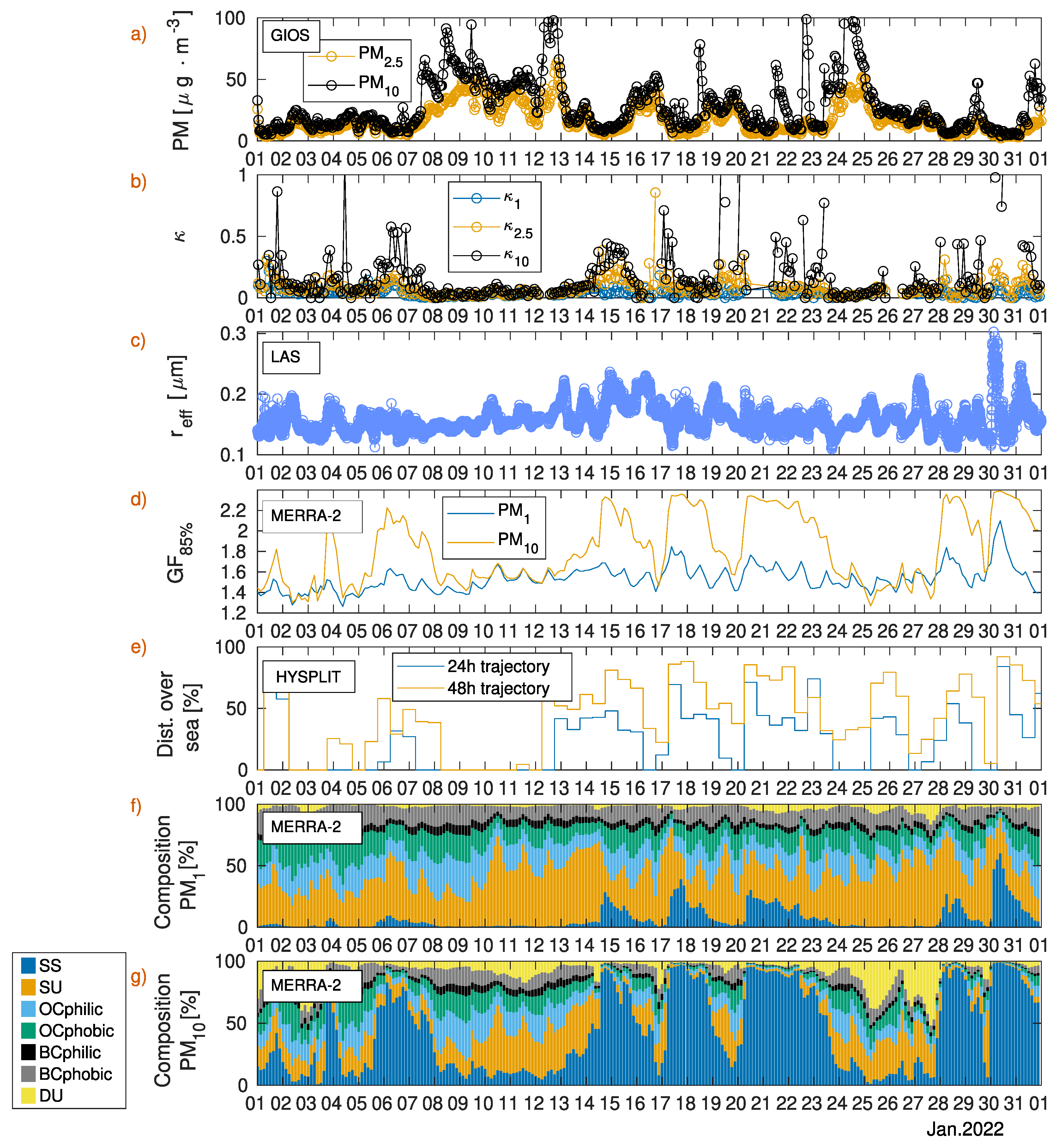
From 26 December, there was a high over Poland, providing sunny and windless weather on 27 December. On 28 December, the high was displaced by the Atlantic low approaching from Great Britain. Together with the Mediterranean low, they caused an increase in wind speed on 28 December, incoming air from south-eastern directions [31,32]. The weather from 28 December (till 6 January) was mainly controlled by the appearance of successive Atlantic lows that favored the influx of warm air, mainly from the south-west and west directions. These lows moved along the northern side of the quasi-stationary high of the Azores. From 30 December, the temperatures were above zero degrees. When the coming air to Poland was from south-west directions the values where increasing from 0 at 27 December to 0.13 on 31 December. During days 26 and 31 December the air pollution was high, the norms of PM, PM where exceeded.
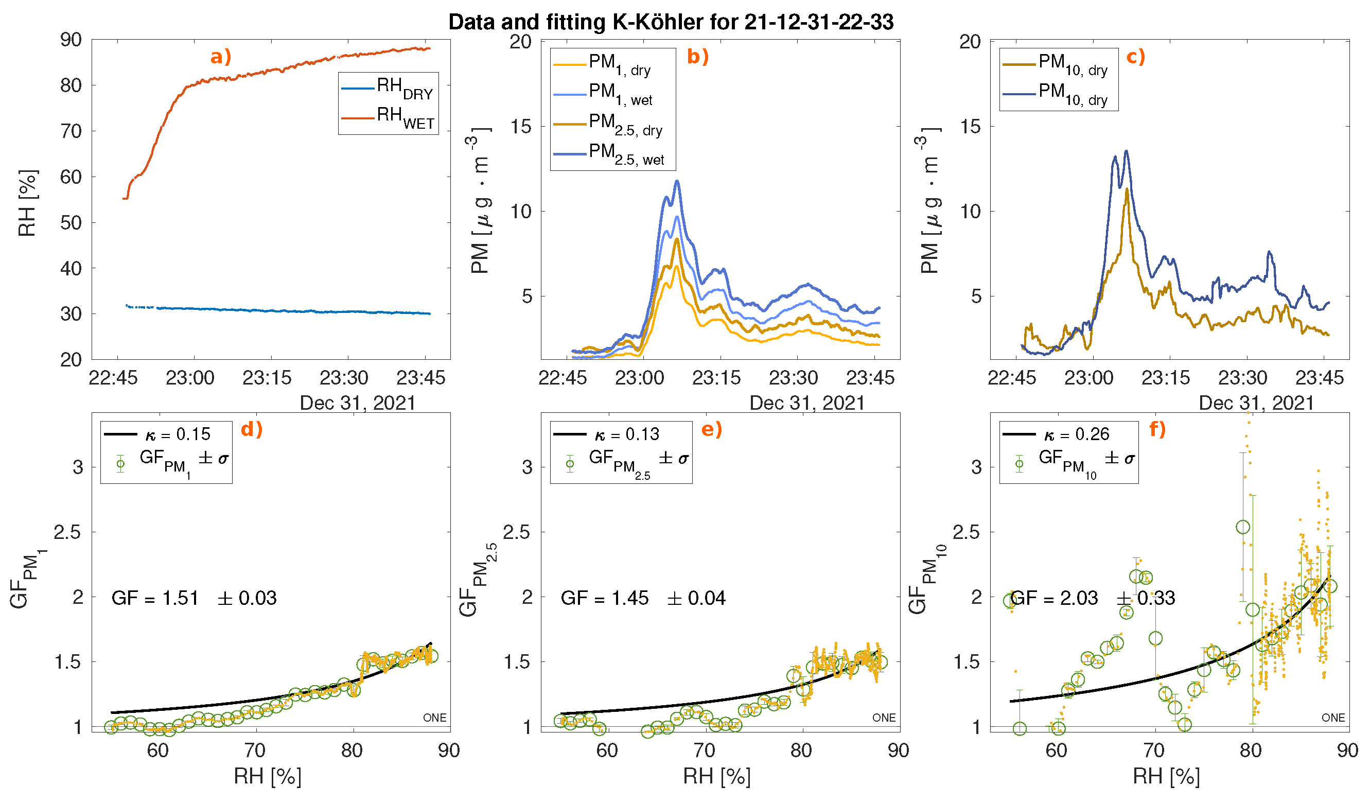
The last performed cycle in 2021 was during the New Year celebration. Before New Years firework shoot the , , where respectively 0.05, 0.08, 0.09. For the last cycle of , and were slightly elevated (0.09, 0.12 and 0.14 respectively). After midnight, the values returned to values similar to before midnight (0.06, 0.07 and 0.09 , , respectively). The Figure A4 show the humidograms for growth factor of PM, PM and PM as well as registered values of PM and RH in ACS 1000. The atmosphere before New Year was clear (PM around 1.5 and PM 2 [g·m]), we observed a jump of PM to 6.5 and PM to 8 [g·m] 6 min after midnight. At that time, the RH in ACS 1000 was 81.5%.
The particulate matter emitted did not show an abnormal change in GF for this cycle. This is in contrast to previously reported works in which fireworks were identified to consist of ion salts, mostly sulfate, potassium and chloride, sodium, and magnesium, which show high hygroscopicity [34,35].
In the subsequent month, January 2022, similar behavior was observed. Whenever the MERRA-2 reanalysis shows more than 50% of sea salt contribution into PM mass the increases from around 0.05 to values greater than 1.0 and the GF for PM from MERRA-2 also increases to values greater than 2.2. When periods such as 8–13 January appear, when the air masses did not pass over sea (the sea salt contribution is low), then the values of are below 0.05. During this period, the concentration of PM were above 25 g·m and PM above 50 g·m.
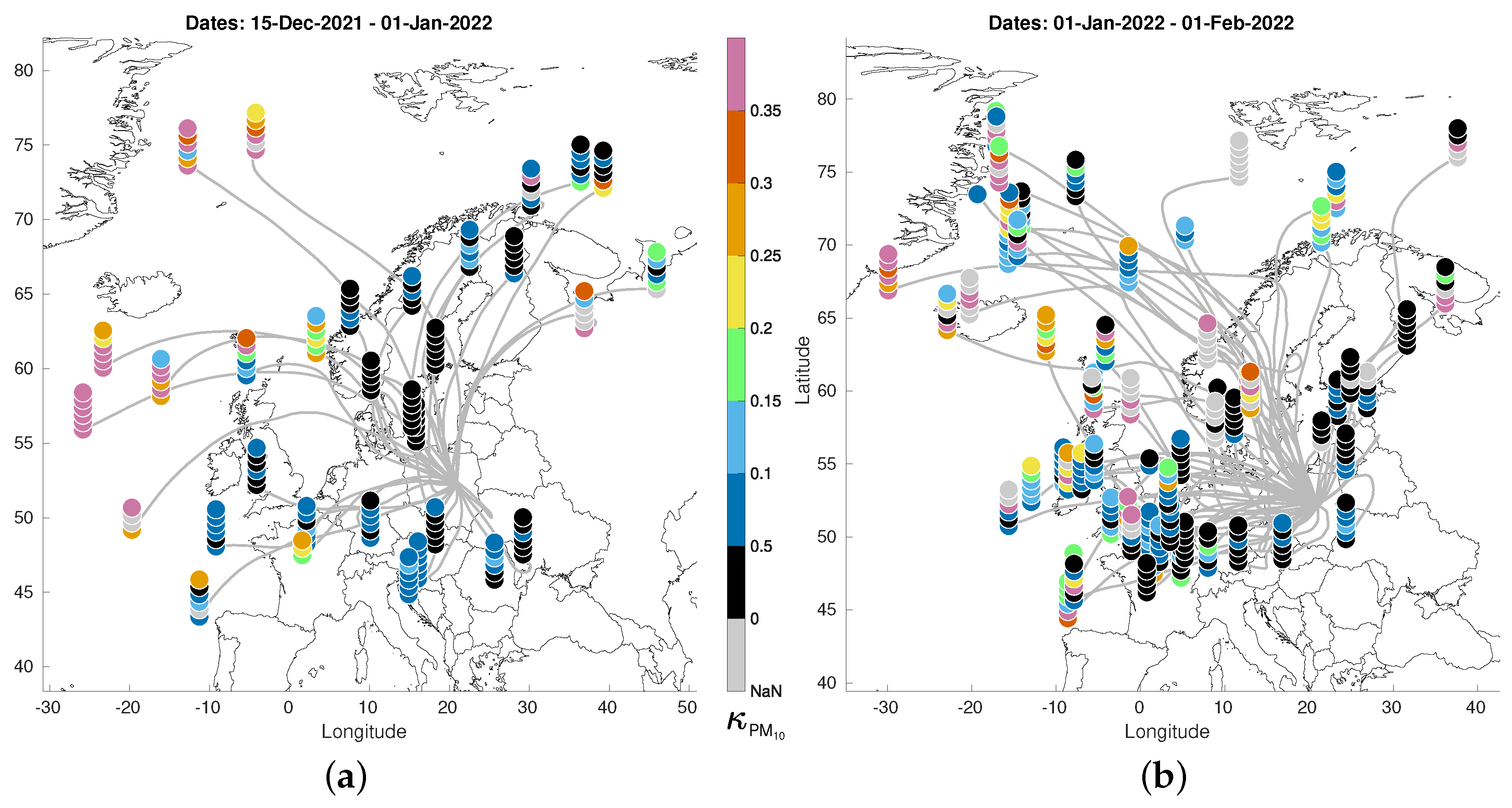
Figure 8 presents the air flow path with the assigned value (denoted by colored circle). The grater the length of the path is the quicker the air parcel was moving towards RTL at Warsaw. Values of above 0.2 are mostly associated with the fast flow of air from the North Atlantic, Northern Sea, Norwegian Sea, or Barents Sea.
4.3.2. Spring 2020 (28 April–5 May, 16 May–24 May)
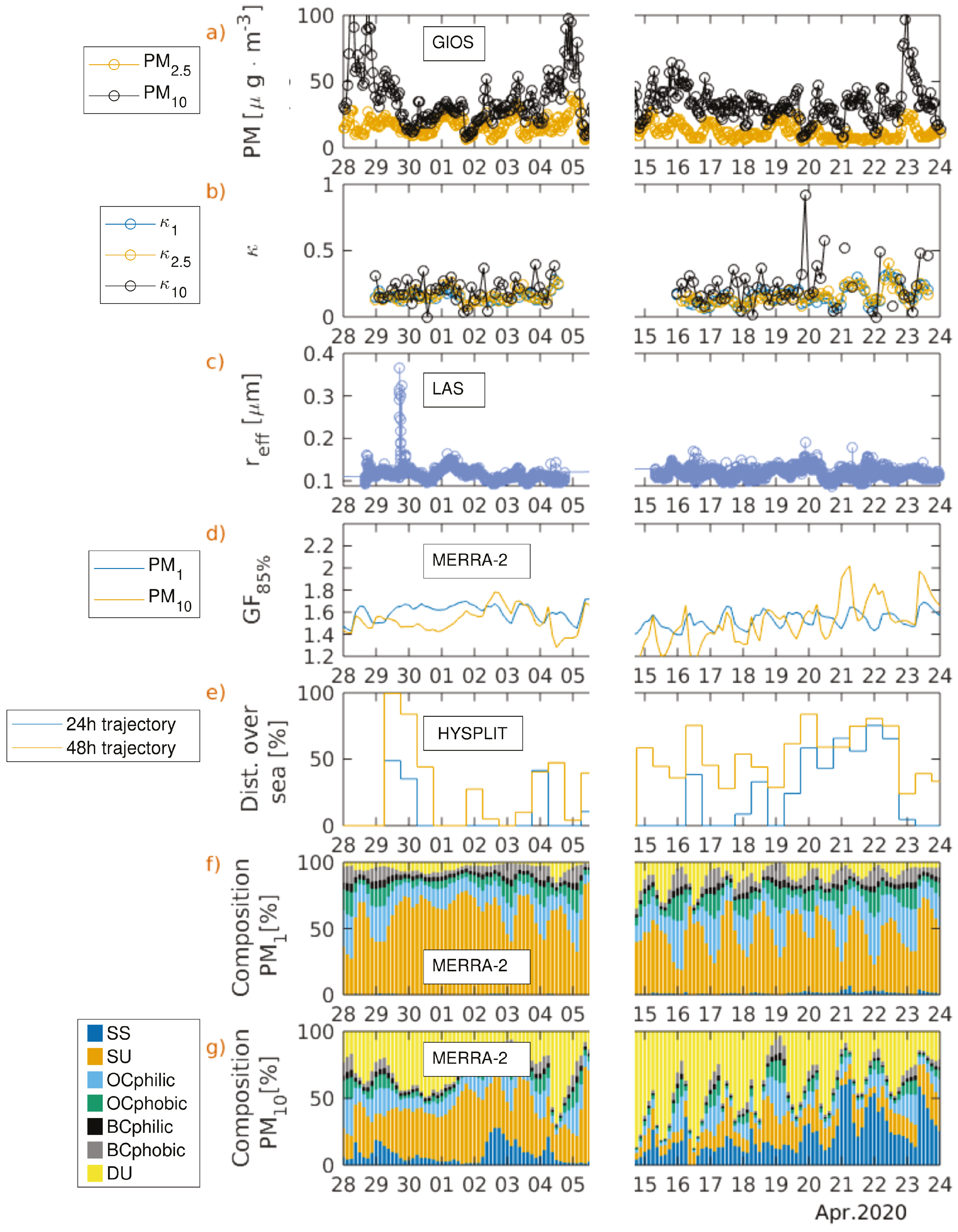
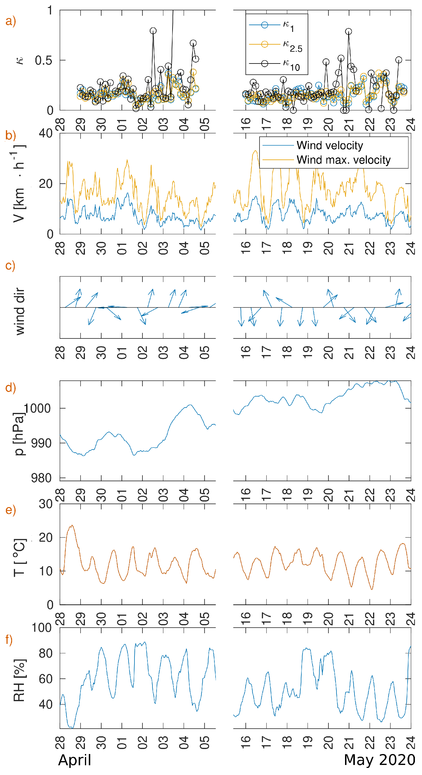
To show the picture of the spring measurements regarding the aerosol hygroscopicity a period was chosen from 28 April to 24 May 2020 (with a break between 5 and 16 May). Figure 9 presents the values for spring 2020 and Figure A5 the meteorological conditions at the RTL station during that time. Obtained values of were oscillating near value 0.2. Most of the time , where having similar values. The events when was greater than 0.4 where occurring only for this was for days 20–24 May.
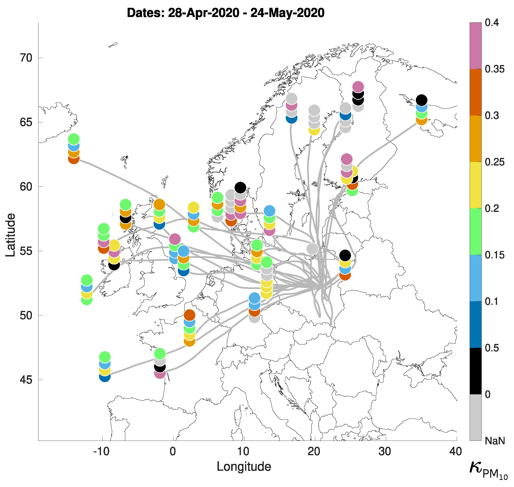
The 24-h mean of the concentrations of PM and PM from the GIOś station did not exceed WHO limits. In the winter case (apart from smog events), the concentrations of PM and PM were similar; in the spring case the lines in Figure 9a are separated, suggesting that there are more large particles (above 2.5 m) in the air aerosol compared to the winter period. The composition of the PM mass is different than in winter. For PM contribution of sulphates is more than , with visible diurnal cycle, black carbon provide less to the total mass than in winter season. However, dust gives a higher contribution to total mas of PM than in winter. Nevertheless MERRA-2 reanalysis show events of sea salt particles in the air there is no visible correlation of it with . Using the HYSPLIT model, the percentage of incoming air over the sea was calculated; the correlation between kappa and distance over the sea is also low. Figure 10 presents what was the path of incoming air to RTL in previous 48 h. There is no specific region for which would be seen that the is grater.
5. Calibrating OPC
As we have shown, the PM values are biased by high RH. To calibrate the OPC we transformed Equation (4) to obtain PM as it would be registered if RH was zero (refereed as PM). The OPC-N3 built-in hygrometer shows lower RH values than those registered by ASC1000. Our guess is that the OPC-N3 hygrometer is near to the control board, which causes heating, leading to underestimation of RH. Therefore first we calibrated the RH from OPC-N3 versus ACS 1000 and then calculated the PM.
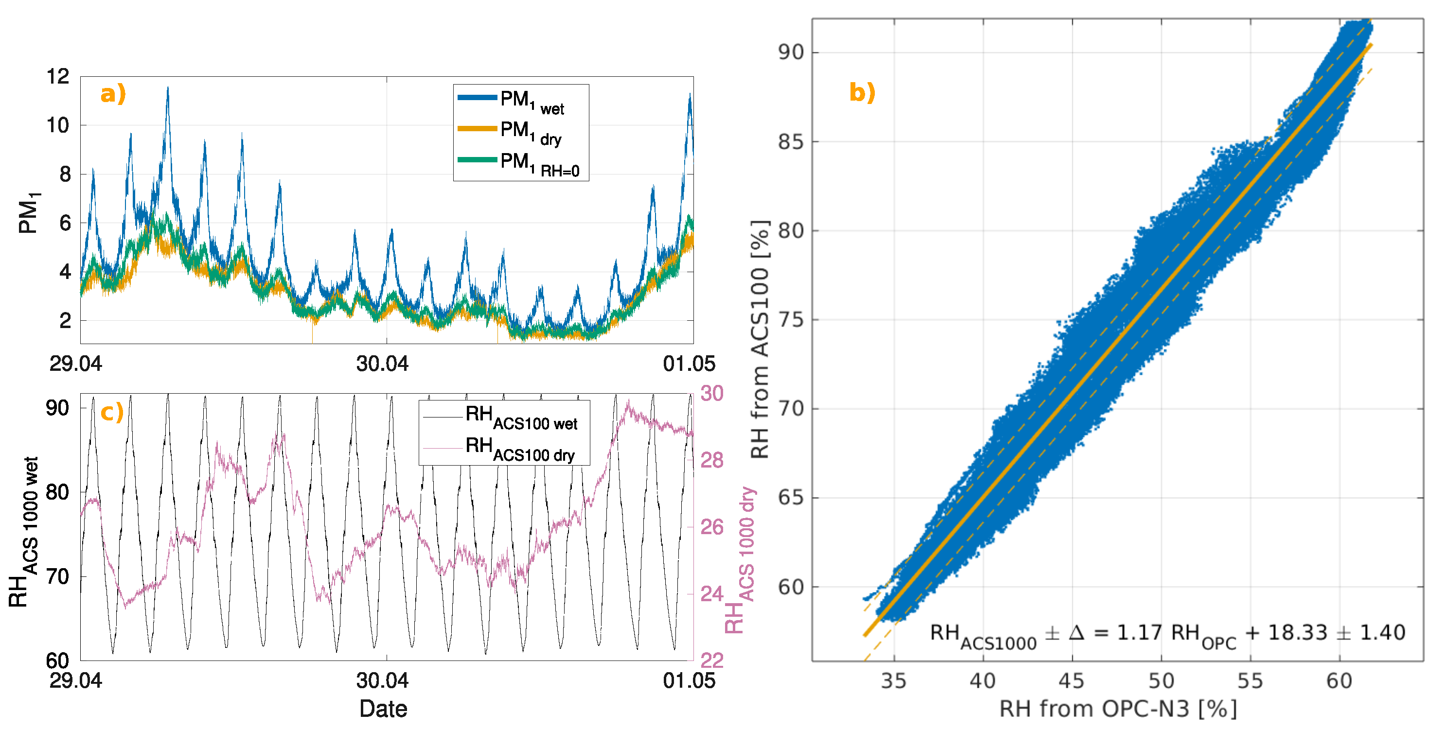
Figure 11b presents relative humidity registered by OPC-N3 versus RH form ACS 1000. For Period nr 1 (Spring 2020), we fit a line to the RH data from OPC-N3 versus ACS 1000 (orange line Figure 11b). We obtained the following fitting:
By transforming Equation (4), we get the formula for PM:
where PM is the PM measured by OPC-N3, RH is the relative humidity from OPC-N3, a and b are the estimated parameters from Equation (7). For calibration we used the mean value for the period 29–30 April 2020 ().
Figure 11 shows the comparison of PM and PM over a period of two days. The upper panel shows the data from OPC-N3 PM (blue color) compared to the PM data from OPC-N3 PM (orange color) and the calibrated PM (green color). Lower panel presents the cycles of RH in ACS100: in pink the RH from dry brunch and in black from the wet brunch.
Figure 11 displays the PM data obtained from both the wet brunch (blue line in panel a) and the dry channel (orange line in panel a). In Figure 11c, the graph illustrates the temporal changes in relative humidity within the wet brunch (depicted by the black line), while the pink line represents the RH in the dry channel.
Analysis of Figure 11 indicates that the PM values measured at high RH, following the proposed correction (green line in Figure 11a), closely resemble the PM levels measured at RH below 30% (orange line in Figure 11a). In particular, on 29 April, PM appeared more hygroscopic compared to 30 April, suggesting that applying the same correction factor () for both days works better for the latter day.
Despite the presence of residual variations with respect to RH after the correction, these fluctuations are considerably smaller.
In our study, the hygroscopicity of the atmospheric aerosol mixture obtained from PM varied from almost 0 to = 0.2. We wanted to know how much differ the values of PM obtained at high ambient RH (where RH denotes = ) with the PM obtained in RH below . We chose three different days 27 December 2020, 29 March 2020 and 4 May 2020 where was respectively 0.01, 0.13 and 0.20. Table A3 shows for those days the PM registered at and at RH = , apart from values in [g· m] the PM is presented as a percentage of value PM. For a day when was 0.01 even for the RH of the error made is within 10%, however, if was 0.13 the error is greater. For = 0.13 the error is bigger than 20% for RH exceeding , in case of RH = 90% the error is 61.33%. For = 0.20 the the error bigger than 20% is already for RH exceeding . When the RH = 90% the obtained values of PM are more than twice bigger than registered in dry conditions.
In addition to checking the error generated by recording PM values without prior drying the air, we wanted to check how correcting the values of PM registered in high RH using helps to improve the results. For each day 27 December 2020, 29 March 2020 and 4 May 2020 we corrected the PM using , the results are shown in the same Table A3. For each day when using closest to the estimated value, the percentage error between the corrected value and the measured PM value was below . In the case of estimated = 0.01 using for correction larger values of caused an underestimation of PM by up to 20%. The biggest errors occur when selecting the wrong kappa for correction when the actual kappa value is large.
6. Summary of the Results
In this work we show that a set of two OPC-N3 and an ACS 1000 can be used to study the hygroscopicity of an aerosol. During three years, we measured (a dimensionless parameter specifying the hygroscopicity of the aerosol [21]) during the months December–June. This were the first measurements of outdoor aerosol hygroscopicity conducted in Poland. Overall registered values of in the spring season (April–July) were higher—, , (, , respectively) than in winter (January–March)—, , (, , respectively). There is a high correlation between and GF calculated from the same PM size: 0.98, 0.97 and 0.89 (PM, PM, PM respectively). Using the GF parameter has better variability, so the error values are not the same magnitude as the given value. For spring, the GF was for PM, PM, PM , , respectively; and for winter it was , , , respectively. We have shown that
- the hygroscopicity parameter () for PM during winter (December–March) is below 0.05. These periods were when pollution was high (PM and PM WHO norms were exceeded). This is likely that the air pollution consists mostly of soot, from home heating systems, which is non-hygroscopic.
- During winter there are events when the hygroscopicity of PM is low and the hygroscopicity of PM is high up to 1. These events are probably associated with fast flow of air masses from the North Atlantic Ocean during low pressure circumstances. The PM mass in more than consists of sea salt particles.
- There is a dependence of on the time of day. During the sun’s operating hours, the values of are statistically higher than in the evening/night.
- During the New Year’s Eve midnight (when the fireworks are shoot) the parameter for PM, PM and PM raised from values 0.05, 0.08, 0.09 to 0.09, 0.12 and 0.14 respectively. We did not observe higher values of during fireworks shooting.
Apart from hygroscopicity measurements we have tested how to correct low-cost particulate matter counters such as OPC-N3 for RH. Our recommendations for performing air quality measurements with the OPC-N3 device without using a dehumidifier:
- The data can be corrected using , however appointing the appropriate kappa for corrections is difficult.
- If one suspect that the aerosol may be hygroscopic, it is worth taking into account the kappa correction, because PM values registered at high RH with respect to those measured in RH may differ more than twice.
- The RH for correction should be taken from a device different from OPC-N3. The RH values from OPC-N3 are significantly lower than ambient and cannot be easily corrected, as the black OPC-N3 body absorbs sun light, changing the amount of bias.
- For cases when is small (for example for winter) registering PM at ambient RH causes a small error up to 10%.
- We do not recommend using PM values from OPC-N3 for ambient RH above without any correction.
7. Conclusions
This study underscores the feasibility of employing OPC-N3 devices alongside an ACS 1000 to evaluate aerosol hygroscopicity, especially in different seasons. Our findings highlight distinct seasonal variations in values, with elevated hygroscopicity observed during spring compared to winter, indicative of varying aerosol compositions and sources.
Crucially, our observations regarding the values of during high pollution periods in winter suggest a prevalence of hydrophobic particles (such as soot), possibly from domestic heating systems. Additionally, meteorological events, such as rapid air mass movements from the North Atlantic Ocean, significantly influenced aerosol hygroscopicity.
The temporal dependency of values throughout the day and the impact of specific events, further emphasize the dynamic nature of aerosol hygroscopicity.
Furthermore, our study provided practical recommendations for correcting low-cost particulate matter counters like OPC-N3 for RH, emphasizing the significance of considering values in correcting aerosol measurements, especially in conditions of varying RH.
In conclusion, this research contributes valuable insights into the understanding of aerosol hygroscopicity patterns in the Polish urban area, emphasizing the importance of seasonal variations, meteorological influences, and the potential for improved correction methods for RH-dependent aerosol measurements.
Author Contributions
Conceptualization K.M.M. and K.N.; methodology, K.N.; formal analysis, K.N.; investigation, K.N.; writing—original draft preparation, K.N.; writing—review and editing, K.N.; supervision, K.M.M. All authors have read and agreed to the published version of the manuscript.
Funding
This research is part of the OPUS project Impact of aerosol on the microphysical, optical and radiation properties of fog, which was funded by the National Science Center grant number UMO-2017/27/B/ST10/00549.
Institutional Review Board Statement
Not applicable.
Informed Consent Statement
Not applicable.
Data Availability Statement
The data presented in this study are available on request from the corresponding author. The data are not publicly available due to ongoing transformation within our Faculty to consolidate information into a single database.
Conflicts of Interest
The authors declare no conflict of interest.
Abbreviations
The following abbreviations are used in this manuscript:
| ACS 1000 | Acoem Aerosol Conditioning System |
| AOD | aerosol optical depth |
| BC | Black carbon |
| DRH | Deliquescent point |
| DU | Dust |
| ERH | Efflorescence point |
| F | F-test (statistics) |
| GF | Growth factor |
| HYSPLIT | Hybrid Single-Particle Lagrangian Integrated Trajectory model |
| Dimensionless parameter proposed by Crilley et al. [21] | |
| IPCC | Intergovernmental Panel on Climate Change |
| LAS | Laser Aerosol Spectrometer |
| MERRA-2 | Modern-Era Retrospective analysis for Research and Applications, Version 2 |
| OC | Organic carbon |
| OPC-N3 | Low-cost optical particle counter developed by Alphasense Ltd. |
| p | p-value (statistics) or pressure [hPa] |
| PM, PM, PM | Particulate matter of diameter less than or equal to |
| 1 m, 2.5 m and 10 m, respectively | |
| PNC | particle number concentration |
| Effective radius | |
| RH | Relative humidity [%] |
| RH | Minimum relative humidity possible to achive with ACS 1000 system |
| RH | Maximum relative humidity possible to achive with ACS 1000 system |
| water density 1.0 [g ·cm] | |
| internal aerosol density parameter set in OPC-N3 sensors at 1.65 [g ·cm] | |
| RTL | Radiative Transfer Labolatory, Geophysic Insitute, Faculty of Physics, |
| University of Warsaw | |
| SE | Standard error |
| SU | Sulfate aerosol |
| SS | Sea salt |
| T | Temperature [°C] |
| UAV | Unmanned aerial vehicle |
| V | Wind [km·h] |
Appendix A. GIOŚ Station Ave. Niepodległości, Warsaw, NOx
Figure A1.
Boxplot of diurnal variation of NO (panel a,c) and of NO (panel b,d) obtained for GIOŚ station Ave. Niepodległości, Warsaw based on data from 2020–2022. Upper panels presents data collected for winter (December–March) lower panels presents data for spring (April–June).
Figure A1.
Boxplot of diurnal variation of NO (panel a,c) and of NO (panel b,d) obtained for GIOŚ station Ave. Niepodległości, Warsaw based on data from 2020–2022. Upper panels presents data collected for winter (December–March) lower panels presents data for spring (April–June).

Appendix B. OPC-N3 Calibration

Table A1.
Linear fit factors y = ax + b used to calibrate OPC-N3 data for PM, PM, PM. Only values of SE needs to be multiplied by .
Table A1.
Linear fit factors y = ax + b used to calibrate OPC-N3 data for PM, PM, PM. Only values of SE needs to be multiplied by .
| Period | Calibration | a ± SE ∗ 10−2 | b ± SE ∗ 10−2 |
|---|---|---|---|
| nr | for | ||
| 1 | PM | 0.64 ± 0.11 | −0.12 ± 1.03 |
| PM | 0.67 ± 0.17 | 0.03 ± 2.00 | |
| PM | 0.57 ± 0.44 | 0.89 ± 6.88 | |
| 2 | PM | 0.85 ± 0.10 | 0.20 ± 0.50 |
| PM | 0.82 ± 0.13 | 0.29 ± 0.81 | |
| PM | 0.79 ± 0.27 | 0.47 ± 1.80 | |
| 3 | PM | 0.88 ± 0.05 | 0.4 ± 0.57 |
| PM | 0.86 ± 0.06 | 0.6 ± 0.79 | |
| PM | 0.84 ± 0.10 | 0.82 ± 1.39 | |
| 4 | PM | 0.40 ± 0.12 | 0.03 ± 0.18 |
| PM | 0.43 ± 0.31 | 0.18 ± 0.78 | |
| PM | 0.24 ± 0.71 | 1.52 ± 3.31 | |
| 5 | PM | 1.22 ± 0.08 | 0.09 ± 0.36 |
| PM | 1.09 ± 0.09 | 0.17 ± 0.51 | |
| PM | 1.00 ± 0.15 | 0.45 ± 0.89 | |
| 6 | PM | 1.24 ± 0.05 | −0.06 ± 0.12 |
| PM | 1.11 ± 0.09 | −0.09 ± 0.27 | |
| PM | 0.81 ± 0.19 | 0.61 ± 0.74 | |
| 7 | PM | 1.23 ± 0.12 | 0.01 ± 0.39 |
| PM | 1.13 ± 0.16 | −0.01 ± 0.63 | |
| PM | 0.75 ± 0.42 | 1.18 ± 2.12 |
Appendix C. Winter 2021–2022
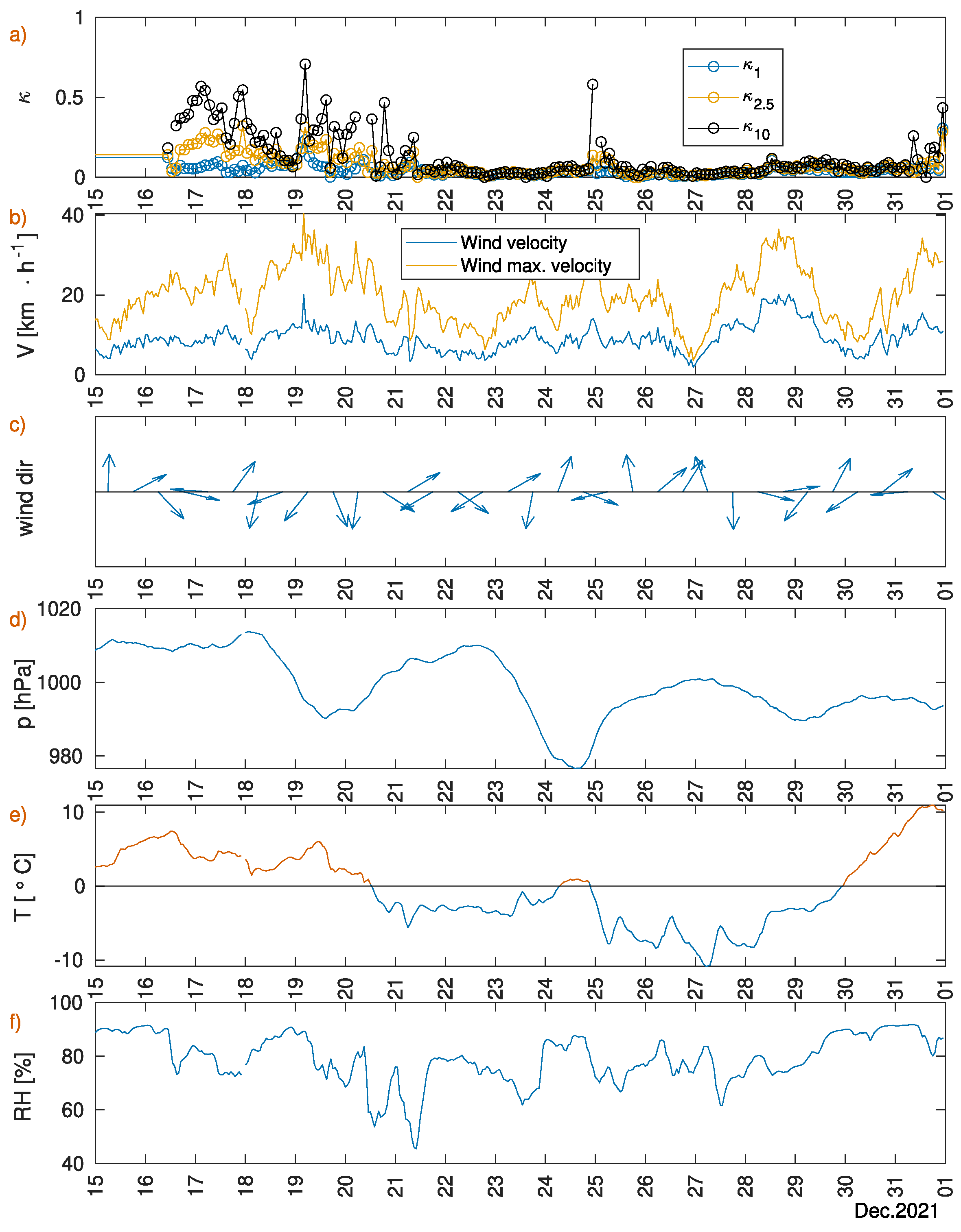
Figure A2.
December 2021: Panels represents changes of variables during winter 2021/2022 case. (a) Kappa obtained from data from ACS 1000 and OPC-N3 in RTL for each cycle. Blue line PM, orange line PM, black line PM. (b) wind velocity (blue line) and wind gusts (orange line), (c) wind direction, (d) pressure, (e) temperature, (f) relative humidity. Panels (b,d–f) presents one hour average from Vaisala WXT 520 instrument, Panels (c) presents 12 h average from Vaisala WXT 520 instrument.

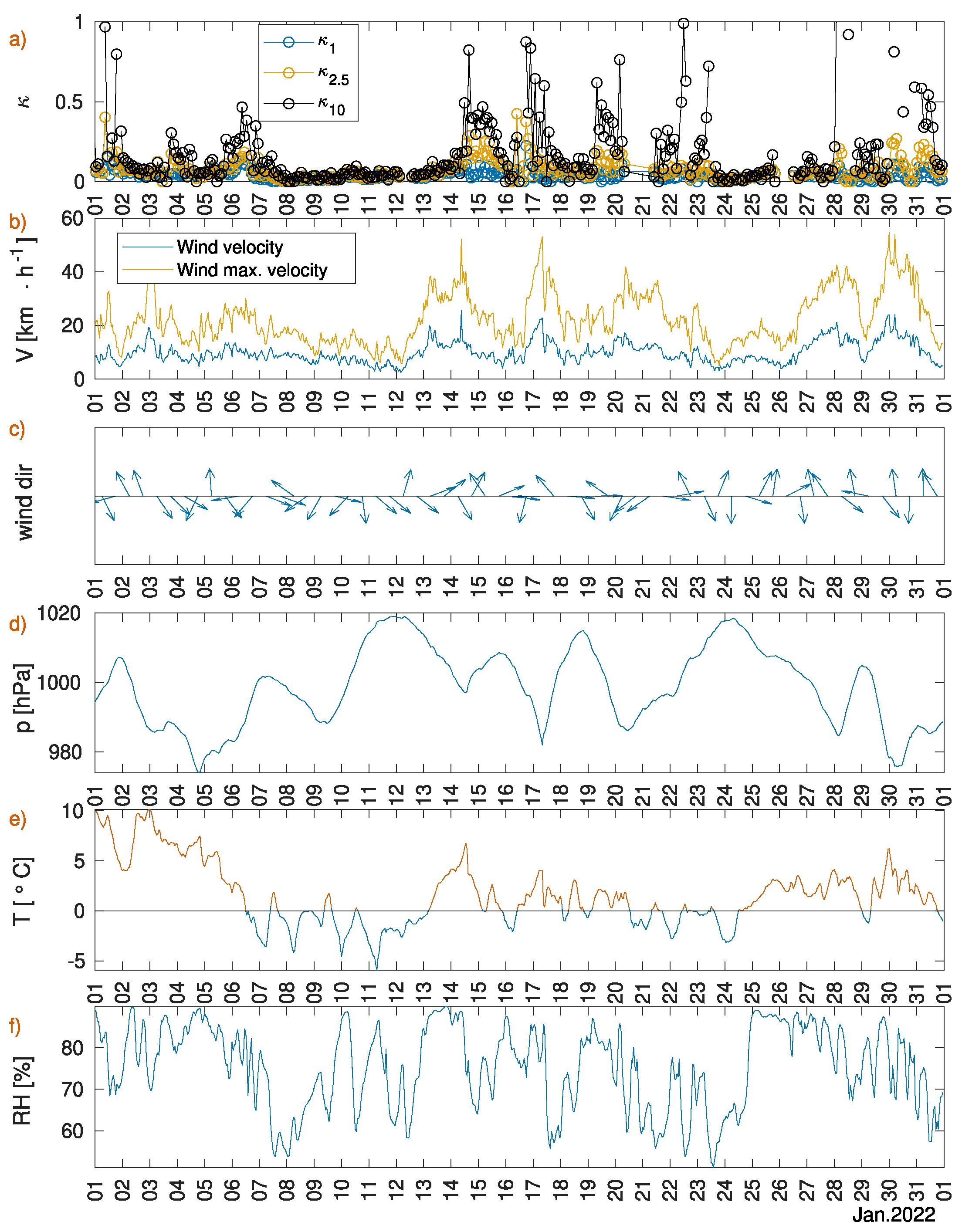
Figure A3.
January 2022: Panels represents changes of variables during winter 2021/2022 case. (a) Kappa obtained from data from ACS 1000 and OPC-N3 in RTL for each cycle. Blue line PM, orange line PM, black line PM. (b) wind velocity (blue line) and wind gusts (orange line), (c) wind direction, (d) pressure, (e) temperature, (f) relative humidity. Panels (b,d–f) presents one hour average from Vaisala WXT 520 instrument, Panels (c) presents 12 h average from Vaisala WXT 520 instrument.

Figure A4.
Figure shows last cycle of the ACS 1000 and registered PM by OPC-N3 in 2021. The change of RH in the ACS 1000 is shown on panel (a), the registered PM, PM are shown in panel (b) and in panel (c) PM (after calibration and applying running average of 12 points). Plots (d–f) presents GF versus RH for one cycle obtained from PM, PM, PM respectively, the black line shows fitted curve defined by Equation (4). Time is in UTC, 23:00 UTC is 00:00 at Warsaw.

Table A2.
Pearson correlation coefficient between variables listed in first column and , GF. Colors divide values by strength of correlation.
Table A2.
Pearson correlation coefficient between variables listed in first column and , GF. Colors divide values by strength of correlation.
| 0.19 | 0.31 | 0.25 | 0.25 | 0.40 | 0.28 | |
| GF MERRA-2 | 0.14 | 0.23 | 0.34 | 0.16 | 0.24 | 0.28 |
| GF MERRA-2 | −0.01 | 0.27 | 0.42 | 0.05 | 0.30 | 0.40 |
| dist sea 24 h | 0.18 | 0.24 | 0.32 | 0.18 | 0.24 | 0.34 |
| dist sea 48 h | 0.15 | 0.28 | 0.39 | 0.16 | 0.31 | 0.39 |
| % SS | −0.01 | 0.26 | 0.41 | 0.04 | 0.29 | 0.39 |
| T | 0.56 | 0.35 | 0.49 | 0.48 | 0.39 | 0.34 |
| p | 0.06 | 0.16 | 0.25 | 0.04 | 0.21 | 0.33 |
| RH | 0.27 | −0.06 | −0.01 | 0.18 | −0.03 | −0.14 |
| V | 0.35 | 0.16 | 0.09 | 0.34 | 0.15 | −0.03 |
| 0.53 | 0.33 | 0.36 | 0.51 | 0.35 | 0.17 | |
| GF | GF | GF | ||||
| statistically insignificant | ||||||
| 0.0 ≤ |r| ≤ 0.2—no correlation | ||||||
| 0.2 < |r| ≤ 0.4—weak correlation | ||||||
| 0.4 < |r| ≤ 0.7—medium correclation | ||||||
| 0.7 < |r| ≤ 0.9—high correlation | ||||||
| 0.9 < |r| ≤ 1.0—very high correlation | ||||||
Appendix D. Spring 2020
Figure A5.
April–May 2020: Panels represents changes of variables during spring 2020 case. (a) Kappa obtained from data from ACS 1000 and OPC-N3 in RTL for each cycle. Blue line PM, orange line PM, black line PM. (b) wind velocity (blue line) and wind gusts (orange line), (c) wind direction, (d) pressure, (e) temperature, (f) relative humidity. Panels (b,d–f) presents one hour average from Vaisala WXT 520 instrument, Panels (c) presents 12 h average from Vaisala WXT 520 instrument.

Appendix E. OPC-N3 Correction
Table A3.
In the Table are presented values of PM registered during specific date by ACS 1000 and OPC-N3. PM refers to data from dry brunch of ACS 1000 where RH was not exceeding and PM refers to PM measured at specific RH listed in each row. Values are given in [g·m] or as a percentage of PM. Columns from 5 to 9 were obtained by applying Equation (8) to data PM with assumption of one of the . At the top of each subtable is presented for which day was created and what was the value of obtained for that day.
| Particulate Matter | = 0.01 | Day: 27 December 2020 | ||||||
|---|---|---|---|---|---|---|---|---|
| RH | PM | PM | ESTIMATED Value Using | |||||
| Measured Value | Measured Value | 0.05 | 0.10 | 0.15 | 0.20 | 0.25 | ||
| 60 % | [g·m] | 4.20 | 4.11 | 4.07 | 3.96 | 3.85 | 3.75 | 3.65 |
| [%] | 2 | −1 | −4 | −6 | −9 | −11 | ||
| 65 % | [g·m] | 4.29 | 4.11 | 4.15 | 4.01 | 3.89 | 3.77 | 3.66 |
| [%] | 4 | 1 | −2 | −6 | −8 | −11 | ||
| 70 % | [g·m] | 4.41 | 4.17 | 4.23 | 4.07 | 3.91 | 3.77 | 3.64 |
| [%] | 6 | 2 | −2 | −6 | −9 | −13 | ||
| 75 % | [g·m] | 4.44 | 4.13 | 4.22 | 4.02 | 3.84 | 3.67 | 3.52 |
| [%] | 8 | 2 | −3 | −7 | −11 | −15 | ||
| 80 % | [g·m] | 4.51 | 4.24 | 4.27 | 4.06 | 3.87 | 3.69 | 3.53 |
| [%] | 6 | 1 | −4 | −9 | −13 | −17 | ||
| 85 % | [g·m] | 4.53 | 4.24 | 4.28 | 4.05 | 3.84 | 3.65 | 3.48 |
| [%] | 7 | 1 | −5 | −9 | −14 | −18 | ||
| 90 % | [g·m] | - | - | - | - | - | - | - |
| [%] | - | - | - | - | - | - | - | |
| Particulate Matter | = 0.13 | Day: 29 March 2020 | ||||||
| RH | PM | PM | ESTIMATED value using | |||||
| Measured value | Measured value | 0.05 | 0.10 | 0.15 | 0.20 | 0.25 | ||
| 60 % | [g·m] | 15.60 | 14.88 | 14.91 | 14.27 | 13.69 | 13.15 | 12.65 |
| [%] | 5 | 0 | −4 | −8 | −12 | −15 | ||
| 65 % | [g·m] | 16.00 | 14.96 | 15.12 | 14.34 | 13.63 | 12.99 | 12.41 |
| [%] | 7 | 1 | −4 | −9 | −13 | −17 | ||
| 70 % | [g·m] | 13.96 | 12.57 | 13.02 | 12.20 | 11.48 | 10.83 | 10.26 |
| [%] | 11 | 4 | −3 | −9 | −14 | −18 | ||
| 75 % | [g·m] | 15.22 | 12.76 | 13.90 | 12.79 | 11.84 | 11.03 | 10.32 |
| [%] | 19 | 9 | 0 | −7 | −14 | −19 | ||
| 80 % | [g·m] | 16.48 | 13.18 | 14.72 | 13.31 | 12.14 | 11.17 | 10.34 |
| [%] | 25 | 12 | 1 | −8 | −15 | −22 | ||
| 85 % | [g·m] | 19.01 | 13.06 | 16.03 | 13.86 | 12.21 | 10.91 | 9.86 |
| [%] | 46 | 23 | 6 | −7 | −16 | −25 | ||
| 90 % | [g·m] | 22.62 | 14.02 | 18.31 | 15.37 | 13.25 | 11.64 | 10.38 |
| [%] | 61 | 31 | 10 | −6 | −17 | −26 | ||
| Particulate Matter | = 0.20 | Day: 4 May 2020 | ||||||
| RH | PM | PM | ESTIMATED value using | |||||
| Measured value | Measured value | 0.05 | 0.10 | 0.15 | 0.20 | 0.25 | ||
| 60 % | [g·m] | 2.05 | 1.90 | 1.96 | 1.87 | 1.79 | 1.72 | 1.66 |
| [%] | 8 | 3 | −2 | −6 | −9 | −13 | ||
| 65 % | [g·m] | 2.87 | 2.53 | 2.72 | 2.59 | 2.46 | 2.35 | 2.25 |
| [%] | 14 | 8 | 2 | −3 | −7 | −11 | ||
| 70 % | [g·m] | 2.87 | 2.32 | 2.68 | 2.52 | 2.37 | 2.24 | 2.13 |
| [%] | 24 | 16 | 9 | 2 | −3 | −8 | ||
| 75 % | [g·m] | 3.81 | 2.83 | 3.48 | 3.20 | 2.96 | 2.76 | 2.58 |
| [%] | 35 | 23 | 13 | 5 | −2 | −9 | ||
| 80 % | [g·m] | 4.15 | 2.76 | 3.69 | 3.31 | 3.01 | 2.76 | 2.54 |
| [%] | 51 | 34 | 20 | 9 | 0 | −8 | ||
| 85 % | [g·m] | 4.92 | 2.60 | 4.13 | 3.56 | 3.13 | 2.79 | 2.52 |
| [%] | 89 | 59 | 37 | 20 | 7 | −3 | ||
| 90 % | [g·m] | 5.73 | 2.62 | 4.59 | 3.83 | 3.28 | 2.88 | 2.56 |
| [%] | 119 | 75 | 46 | 25 | 10 | −2 | ||
References
- IPCC. Summary for Policymakers. In Climate Change 2013: The Physical Science Basis. Contribution of Working Group I to the Fifth Assessment Report of the Intergovernmental Panel on Climate Change; Stocker, T., Qin, D., Plattner, G.K., Tignor, M., Allen, S., Boschung, J., Nauels, A., Xia, Y., Bex, V., Midgley, P., Eds.; Cambridge University Press: Cambridge, UK; New York, NY, USA, 2013; Book Section SPM; pp. 1–30. [Google Scholar] [CrossRef]
- Laden, F.; Neas, L.; Dockery, D.; Schwartz, J. Association of Fine Particulate Matter from Different Sources with Daily Mortality in Six U.S. Cities. Environ. Health Perspect. 2000, 108, 941–947. [Google Scholar] [CrossRef] [PubMed]
- Maciejewska, K. Short-term impact of PM2.5, PM10, and PMc on mortality and morbidity in the agglomeration of Warsaw, Poland. Air Qual. Atmos. Health 2020, 13, 659–672. [Google Scholar] [CrossRef]
- European Union. Directive 2008/50/EC of the European Parliament and of the Council of 21 May 2008 on ambient air quality and cleaner air for Europe. Off. J. Eur. Union 2008, L152, 1–44. [Google Scholar]
- World Health Organization. WHO Air Quality Guidelines for Particulate Matter, Ozone, Nitrogen Dioxide and Sulfur Dioxide. 2006. Available online: https://apps.who.int/iris/handle/10665/69477 (accessed on 13 November 2023).
- European Environment Agency. Air Quality in Europe — 2020 Report No 9/2020; Technical Report; European Environment Agency: Copenhagen, Denmark, 2020. [Google Scholar]
- WMO/GAW. Aerosol Measurement Procedures Guidelines and Recommendations; World Meteorological Organization: Geneva, Switzerland, 2003. [Google Scholar]
- Zieger, P.; Fierz-Schmidhauser, R.; Gysel, M.; Ström, J.; Henne, S.; Yttri, K.E.; Baltensperger, U.; Weingartner, E. Effects of relative humidity on aerosol light scattering in the Arctic. Atmos. Chem. Phys. 2010, 10, 3875–3890. [Google Scholar] [CrossRef]
- Zieger, P.; Väisänen, O.; Corbin, J.; Partridge, D.; Bastelberger, S.; Mousavi-Fard, M.; Rosati, B.; Gysel, M.; Krieger, U.; Leck, C.; et al. Revising the hygroscopicity of inorganic sea salt particles. Nat. Commun. 2017, 8, 15883. [Google Scholar] [CrossRef] [PubMed]
- Petters, M.D.; Kreidenweis, S.M. A single parameter representation of hygroscopic growth and cloud condensation nucleus activity. Atmos. Chem. Phys. 2007, 7, 1961–1971. [Google Scholar] [CrossRef]
- Moore, R.H.; Ziemba, L.D.; Dutcher, D.; Beyersdorf, A.J.; Chan, K.; Crumeyrolle, S.; Raymond, T.M.; Thornhill, K.L.; Winstead, E.L.; Anderson, B.E. Mapping the Operation of the Miniature Combustion Aerosol Standard (Mini-CAST) Soot Generator. Aerosol Sci. Technol. 2014, 48, 467–479. [Google Scholar] [CrossRef]
- Titos, G.; Cazorla, A.; Zieger, P.; Andrews, E.; Lyamani, H.; Granados-Muñoz, M.i.; Olmo, F.; Arboledas, L. Effect of hygroscopic growth on the aerosol light-scattering coefficient: A review of measurements, techniques and error sources. Atmos. Environ. 2016, 141, 494–507. [Google Scholar] [CrossRef]
- Vlasenko, S.S.; Su, H.; Pöschl, U.; Andreae, M.O.; Mikhailov, E.F. Tandem configuration of differential mobility and centrifugal particle mass analysers for investigating aerosol hygroscopic properties. Atmos. Meas. Tech. 2017, 10, 1269–1280. [Google Scholar] [CrossRef]
- Wise, M.E.; Martin, S.T.; Russell, L.M.; Buseck, P.R. Water Uptake by NaCl Particles Prior to Deliquescence and the Phase Rule. Aerosol Sci. Technol. 2008, 42, 281–294. [Google Scholar] [CrossRef]
- Nurowska, K.; Mohammadi, M.; Malinowski, S.; Markowicz, K. Applicability of the low-cost OPC-N3 optical particle counter for microphysical measurements of fog. Atmos. Meas. Tech. 2023, 16, 2415–2430. [Google Scholar] [CrossRef]
- Kaur, K.; Kelly, K.E. Performance evaluation of the Alphasense OPC-N3 and Plantower PMS5003 sensor in measuring dust events in the Salt Lake Valley, Utah. Atmos. Meas. Tech. 2023, 16, 2455–2470. [Google Scholar] [CrossRef]
- Sousan, S.; Koehler, K.; Hallett, L.; Peters, T.M. Evaluation of the Alphasense optical particle counter (OPC-N2) and the Grimm portable aerosol spectrometer (PAS-1.108). Aerosol Sci. Technol. 2016, 50, 1352–1365. [Google Scholar] [CrossRef] [PubMed]
- Samad, A.; Melchor Mimiaga, F.E.; Laquai, B.; Vogt, U. Investigating a Low-Cost Dryer Designed for Low-Cost PM Sensors Measuring Ambient Air Quality. Sensors 2021, 21, 804. [Google Scholar] [CrossRef]
- Sousan, S.; Regmi, S.; Park, Y.M. Laboratory Evaluation of Low-Cost Optical Particle Counters for Environmental and Occupational Exposures. Sensors 2021, 21, 4146. [Google Scholar] [CrossRef]
- Dubey, R.; Patra, A.K.; Joshi, J.; Blankenberg, D.; Kolluru, S.S.R.; Madhu, B.; Raval, S. Evaluation of low-cost particulate matter sensors OPC N2 and PM Nova for aerosol monitoring. Atmos. Pollut. Res. 2022, 13, 101335. [Google Scholar] [CrossRef]
- Crilley, L.R.; Shaw, M.; Pound, R.; Kramer, L.J.; Price, R.; Young, S.; Lewis, A.C.; Pope, F.D. Evaluation of a low-cost optical particle counter (Alphasense OPC-N2) for ambient air monitoring. Atmos. Meas. Tech. 2018, 11, 709–720. [Google Scholar] [CrossRef]
- Bílek, J.; Bílek, O.; Maršolek, P.; Buček, P. Ambient Air Quality Measurement with Low-Cost Optical and Electrochemical Sensors: An Evaluation of Continuous Year-Long Operation. Environments 2021, 8, 114. [Google Scholar] [CrossRef]
- Dubey, R.; Patra, A.K.; Joshi, J.; Blankenberg, D.; Nazneen. Evaluation of vertical and horizontal distribution of particulate matter near an urban roadway using an unmanned aerial vehicle. Sci. Total Environ. 2022, 836, 155600. [Google Scholar] [CrossRef]
- Hagan, D.H.; Kroll, J.H. Assessing the accuracy of low-cost optical particle sensors using a physics-based approach. Atmos. Meas. Tech. 2020, 13, 6343–6355. [Google Scholar] [CrossRef]
- Air Quality Portal of the Chief Inspectorate of Environmental Protection— Measurement Data Archives. Available online: https://powietrze.gios.gov.pl/pjp/current/station_details/archive/530?lang=en (accessed on 5 September 2023).
- Global Modeling and Assimilation Office. MERRA2 tavg1_2d_aer_Nx: 2d,1-Hourly, Time-Averaged, Single-Level, Assimilation, Aerosol Diagnostics, Version 5.12.4. 2015. Available online: https://disc.gsfc.nasa.gov/datasets/M2T1NXAER_5.12.4/summary (accessed on 31 August 2023).
- MERRA-2 Frequently Asked Questions. Available online: https://gmao.gsfc.nasa.gov/reanalysis/MERRA-2/FAQ/ (accessed on 5 September 2023).
- Chin, M.; Ginoux, P.; Kinne, S.; Torres, O.; Holben, B.N.; Duncan, B.N.; Martin, R.V.; Logan, J.A.; Higurashi, A.; Nakajima, T. Tropospheric Aerosol Optical Thickness from the GOCART Model and Comparisons with Satellite and Sun Photometer Measurements. J. Atmos. Sci. 2002, 59, 461–483. [Google Scholar] [CrossRef]
- Seber, G.; Wild, C. Nonlinear Regression; Wiley Series in Probability and Statistics; Wiley: Hoboken, NJ, USA, 2003. [Google Scholar]
- Lundgren, D.A. Atmospheric Aerosol Composition and Concentration as a Function of Particle Size and of Time. J. Air Pollut. Control. Assoc. 1970, 20, 603–608. [Google Scholar] [CrossRef] [PubMed]
- Klejnowski, R.; Olędzki, R.; Ostrowski, M. Weatherman Commentary. Available online: https://meteo.icm.edu.pl/komentarze (accessed on 5 September 2023).
- Weather Service of the Polish Institute of Meteorology and Water Management—National Research Institute. Available online: http://meteo.imgw.pl/ (accessed on 5 September 2023).
- Natural Earth-Free Vector and Raster Map Data. Available online: https://www.naturalearthdata.com/downloads/10m-physical-vectors/10m-ocean/ (accessed on 5 September 2023).
- ten Brink, H.; Henzing, B.; Otjes, R.; Weijers, E. Visibility in the Netherlands during New Year’s fireworks: The role of soot and salty aerosol products. Atmos. Environ. 2018, 173, 289–294. [Google Scholar] [CrossRef]
- Drewnick, F.; Hings, S.S.; Curtius, J.; Eerdekens, G.; Williams, J. Measurement of fine particulate and gas-phase species during the New Year’s fireworks 2005 in Mainz, Germany. Atmos. Environ. 2006, 40, 4316–4327. [Google Scholar] [CrossRef]
Figure 1.
Figure shows one cycle of the ACS 1000 and registered PM by OPC-N3 from which was calculated . The change of RH in the ACS 1000 is shown on panel (a), the registered PM, PM are shown in panel (b) and in panel (c) PM (after calibration and applying running average of 12 points). Plots (d–f) presents GF versus RH for one cycle obtained from PM, PM, PM respectively, the black line shows fitted curve defined by Equation (4). Pink oval presents a jump in GF indicating DRH point which occured at RH = 84%.

Figure 2.
Figure represents steps performed to calculate GF for each cycle. (a) First, the region where RH was up to 5 percentile was calculated (blue region). (b) The PM(t) was calculated. (c) The PM(t) was calculated as a difference between PM(t) and PM (t).
Figure 2.
Figure represents steps performed to calculate GF for each cycle. (a) First, the region where RH was up to 5 percentile was calculated (blue region). (b) The PM(t) was calculated. (c) The PM(t) was calculated as a difference between PM(t) and PM (t).

Figure 3.
Daily average obtained for months between December and June, for years 2020–2022. Panel (a) calculation done using PM, (b) PM and (c) PM. The dashed line presents level = 0.05.
Figure 3.
Daily average obtained for months between December and June, for years 2020–2022. Panel (a) calculation done using PM, (b) PM and (c) PM. The dashed line presents level = 0.05.

Figure 4.
Daily average GF obtained for months between December and June, for years 2020–2022. Panel (a) calculation done using PM, (b) PM and (c) PM. The dashed line presents the level of GF = .
Figure 4.
Daily average GF obtained for months between December and June, for years 2020–2022. Panel (a) calculation done using PM, (b) PM and (c) PM. The dashed line presents the level of GF = .

Figure 5.
Boxplot presenting 3 h averaged mean of obtained from PM (a,d), PM(b,e), PM (c,f) for winter months upper panels, for spring bottom panels. The central line indicates the median, the ‘x’ symbol indicates the mean.
Figure 5.
Boxplot presenting 3 h averaged mean of obtained from PM (a,d), PM(b,e), PM (c,f) for winter months upper panels, for spring bottom panels. The central line indicates the median, the ‘x’ symbol indicates the mean.

Figure 6.
December 2021: The panels represent changes of: (a) PM (orange line) and PM (black line) from GIOŚ station located 1.74 km from RTL; (b) obtained from ACS 1000 and OPC-N3 data in RTL for each cycle. Blue line PM, orange line PM, black line PM; (c) effective radius of particles measured by the LAS instrument; (d) GF for RH 85% obtained from MERRA-2; (e) percentage over the sea of air back trajectory obtained from HYSPLIT model, in the panel (f,g) is presented the mass contribution of DU—dust, SS—sea salt, OC—organic carbon, BC—black carbon, SO—sulfate aerosol to the PM and PM respectively obtained from MERRA-2.

Figure 7.
January 2022: The panels represent changes of: (a) PM (orange line) and PM (black line) from GIOŚ station located 1.74 km from RTL; (b) obtained from ACS 1000 and OPC-N3 data in RTL for each cycle. Blue line PM, orange line PM, black line PM; (c) effective radius of particles measured by the LAS instrument; (d) GF for RH 85% obtained from MERRA-2; (e) percentage over the sea of air back trajectory obtained from HYSPLIT model, in the panel (f,g) is presented the mass contribution of DU—dust, SS—sea salt, OC—organic carbon, BC—black carbon, SO—sulfate aerosol to the PM and PM respectively obtained from MERRA-2.

Figure 8.
Gray lines represents the back trajectories calculated, for 0000UTC and 1200UTC, using HYSPLIT ending at 500 m a.s.l. at RTL. The origin of air (48 h prior) observed over the RTL at Warsaw is marked by the lower dot in the stuck. Each stuck point represents the measurements for the period closest to the simulation of air flow from this region. Two plots represent, respectively, (a) December 2021 and (b) January 2022.

Figure 9.
April–May 2020: The panels represent changes of: (a) PM (orange line) and PM (black line) of the GIOŚ station located 1.74 km from RTL; (b) obtained from the ACS 1000 and OPC-N3 data in RTL for each cycle. Blue line PM, orange line PM, black line PM; (c) effective radius of particles measured by the LAS instrument; (d) GF for RH 85% obtained from MERRA-2; (e) percentage over the sea of air back trajectory obtained from HYSPLIT model, in the panel (f,g) is presented the mass contribution of DU—dust, SS—sea salt, OC—organic carbon, BC—black carbon, SO—sulfate aerosol to the PM and PM respectively obtained from MERRA-2.

Figure 10.
Gray lines represents the back trajectories calculated, for 0000UTC and 1200UTC, using HYSPLIT ending at 500 m a.s.l. at RTL. The origin of air (48 h prior) observed over the RTL at Warsaw is marked by the lower dot in the stuck. Each dot on the stuck represents the measurements for the period closest to the simulation of air flow from this region.

Figure 11.
(a) PM, PM and PM obtained from PM for 29 April–1 May 2020; (b) RH from OPC-N3 versus RH from ACS 1000 for Period nr 1 (spring 2020); (c) RH from ACS 1000 for 29 April–1 May 2020.
Figure 11.
(a) PM, PM and PM obtained from PM for 29 April–1 May 2020; (b) RH from OPC-N3 versus RH from ACS 1000 for Period nr 1 (spring 2020); (c) RH from ACS 1000 for 29 April–1 May 2020.

Table 1.
GF at different RH for OC, BC, SU, SS [28].
Table 1.
GF at different RH for OC, BC, SU, SS [28].
| RH [%] | 0 | 50 | 70 | 80 | 90 | 95 | 99 |
|---|---|---|---|---|---|---|---|
| GF | 1.0 | 1.4 | 1.5 | 1.6 | 1.8 | 1.9 | 2.2 |
| GF | 1.0 | 1.2 | 1.4 | 1.5 | 1.6 | 1.8 | 2.2 |
| GF | 1.0 | 1.0 | 1.0 | 1.2 | 1.3 | 1.5 | 1.8 |
| GF | 1.0 | 1.6 | 1.8 | 2.0 | 2.4 | 2.9 | 4.8 |
Table 2.
Periods in which the data about hygroscopicity were collected by ACS 1000 and OPC-N3. When the setting of ACS 1000 was changed, a new calibration of OPC-N3 was performed.
Table 2.
Periods in which the data about hygroscopicity were collected by ACS 1000 and OPC-N3. When the setting of ACS 1000 was changed, a new calibration of OPC-N3 was performed.
| Period | Calibration Performed | Begining | Ending |
|---|---|---|---|
| nr | for RH [%] Below: | [YYYY.MM.DD] | [YYYY.MM.DD] |
| 1 | 60 | 2020.03.26 | 2020.05.23 |
| 2 | 55 | 2020.12.17 | 2021.01.05 |
| 3 | 50 | 2021.01.06 | 2021.01.17 |
| 4 | 60 | 2021.06.04 | 2021.06.13 |
| 5 | 50 | 2021.12.16 | 2022.01.20 |
| 6 | 50 | 2022.01.20 | 2022.02.28 |
| 7 | 50 | 2022.03.01 | 2022.03.15 |
Table 3.
Pearson correlation coefficient between variables listed in first column and row (, GF calculated from PM, PM, PM). Colors divide values by strength of correlation. All correlations have a p-value lower than the assumed statistical significance .
Table 3.
Pearson correlation coefficient between variables listed in first column and row (, GF calculated from PM, PM, PM). Colors divide values by strength of correlation. All correlations have a p-value lower than the assumed statistical significance .
| 1.00 | ||||||
| 0.78 | 1.00 | |||||
| 0.38 | 0.63 | 1.00 | ||||
| 0.98 | 0.76 | 0.36 | 1.00 | |||
| 0.77 | 0.97 | 0.61 | 0.77 | 1.00 | ||
| 0.39 | 0.62 | 0.89 | 0.38 | 0.62 | 1.00 | |
| 0.9 < |r| ≤ 1.0—very high correlation | ||||||
| 0.7 < |r| ≤ 0.9—high correlation | ||||||
| 0.4 < |r| ≤ 0.7—medium correlation | ||||||
| 0.2 < |r| ≤ 0.4—weak correlation | ||||||
| 0.0 ≤ |r| ≤ 0.2—no correlation | ||||||
Table 4.
Mean values of GF and with their standard deviations calculated for PM, PM, PM for winter and spring season for years 2020–2022.
Table 4.
Mean values of GF and with their standard deviations calculated for PM, PM, PM for winter and spring season for years 2020–2022.
| Season | Year | |||
|---|---|---|---|---|
| winter (January–March) | 2020 | 0.04 ± 0.04 | 0.05 ± 0.05 | 0.06 ± 0.07 |
| 2021 | 0.04 ± 0.03 | 0.05 ± 0.07 | 0.08 ± 0.13 | |
| 2022 | 0.04 ± 0.05 | 0.07 ± 0.08 | 0.16 ± 0.20 | |
| Over all years | 0.04 ± 0.04 | 0.06 ± 0.07 | 0.12 ± 0.17 | |
| spring (April–July) | 2020 | 0.14 ± 0.15 | 0.15 ± 0.15 | 0.15 ± 0.15 |
| 2021 | 0.11 ± 0.09 | 0.09 ± 0.09 | 0.09 ± 0.09 | |
| 2022 | ||||
| Over all years | 0.13 ± 0.13 | 0.13 ± 0.13 | 0.13 ± 0.13 | |
| Season | Year | GF | GF | GF |
| winter (January–March) | 2020 | 1.16 ± 0.15 | 1.19 ± 0.16 | 1.22 ± 0.29 |
| 2021 | 1.14 ± 0.12 | 1.21 ± 0.26 | 1.35 ± 0.63 | |
| 2022 | 1.16 ± 0.13 | 1.30 ± 0.30 | 1.71 ± 0.87 | |
| Over all years | 1.16 ± 0.13 | 1.25 ± 0.27 | 1.51 ± 0.76 | |
| spring (April–July) | 2020 | 1.58 ± 0.26 | 1.63 ± 0.26 | 1.63 ± 0.26 |
| 2021 | 1.43 ± 0.14 | 1.38 ± 0.14 | 1.38 ± 0.14 | |
| 2022 | ||||
| Over all years | 1.52 ± 0.23 | 1.53 ± 0.23 | 1.53 ± 0.23 |
Disclaimer/Publisher’s Note: The statements, opinions and data contained in all publications are solely those of the individual author(s) and contributor(s) and not of MDPI and/or the editor(s). MDPI and/or the editor(s) disclaim responsibility for any injury to people or property resulting from any ideas, methods, instructions or products referred to in the content. |
© 2023 by the authors. Licensee MDPI, Basel, Switzerland. This article is an open access article distributed under the terms and conditions of the Creative Commons Attribution (CC BY) license (https://creativecommons.org/licenses/by/4.0/).
Share and Cite
MDPI and ACS Style
Nurowska, K.; Markowicz, K.M. Determination of Hygroscopic Aerosol Growth Based on the OPC-N3 Counter. Atmosphere 2024, 15, 61. https://doi.org/10.3390/atmos15010061
AMA Style
Nurowska K, Markowicz KM. Determination of Hygroscopic Aerosol Growth Based on the OPC-N3 Counter. Atmosphere. 2024; 15(1):61. https://doi.org/10.3390/atmos15010061
Chicago/Turabian StyleNurowska, Katarzyna, and Krzysztof M. Markowicz. 2024. "Determination of Hygroscopic Aerosol Growth Based on the OPC-N3 Counter" Atmosphere 15, no. 1: 61. https://doi.org/10.3390/atmos15010061
Note that from the first issue of 2016, this journal uses article numbers instead of page numbers. See further details here.