
Spectral Clustering of CRISM Datasets in Jezero Crater Using UMAP and k-Means
by
 , and
, and
Alexander Pletl
1,
Michael Fernandes
1,
Nicolas Thomas
2,
Angelo Pio Rossi
3 and
Benedikt Elser
1,* 1
Technologie Campus Grafenau, Technische Hochschule Deggendorf, 94481 Grafenau, Germany
2
Physikalisches Institut, University of Bern, 3012 Bern, Switzerland
3
Department of Physics and Earth Sciences, Constructor University, 28759 Bremen, Germany
*
Author to whom correspondence should be addressed.
Remote Sens. 2023, 15(4), 939; https://doi.org/10.3390/rs15040939
Submission received: 22 December 2022
/
Revised: 30 January 2023
/
Accepted: 2 February 2023
/
Published: 8 February 2023
Abstract
:In this paper, we expand upon our previous research on unsupervised learning algorithms to map the spectral parameters of the Martian surface. Previously, we focused on the VIS-NIR range of hyperspectral data from the CRISM imaging spectrometer instrument onboard NASA’s Mars Reconnaissance Orbiter to relate to other correspondent imager data sources. In this study, we generate spectral cluster maps on a selected CRISM datacube in a NIR range of 1050–2550 nm. This range is suitable for identifying most dominate mineralogy formed in ancient wet environment such as phyllosilicates, pyroxene and smectites. In the machine learning community, the UMAP method for dimensionality reduction has recently gained attention because of its computing efficiency and speed. We apply this algorithm in combination with k-Means to data from Jezero Crater. Such studies of Jezero Crater are of priority to support the planning of the current NASA’s Perseversance rover mission. We compare our results with other methodologies based on a suitable metric and can identify an optimal cluster size of six for the selected datacube. Our proposed approach outperforms comparable methods in efficiency and speed. To show the geological relevance of the different clusters, the so-called “summary products” derived from the hyperspectral data are used to correlate each cluster with its mineralogical properties. We show that clustered regions relate to different mineralogical compositions (e.g., carbonates and pyroxene). Finally the generated spectral cluster map shows a qualitatively strong resemblance with a given manually compositional expert map. As a conclusion, the presented method can be implemented for automated region-based analysis to extend our understanding of Martian geological history.
1. Introduction
A prominent instrument to acquire spectral data from orbit to determine mineralogical properties of specific areas is the CRISM [1] hyperspectral imaging spectrometer onboard NASA’s Mars Reconnaissance Orbiter (MRO). In particular, the area of Nili Fossea including Jezero Crater has been extensively covered. The data indicate mineralogical structures formed in ancient wet environments and therefore supports the 2020 Perserverance rover mission goals.
The planetary geologic mapping process itself relies on basic geometric and stratigraphic principles, historically limited by the availability of image and topographic data. Such process has been greatly aided in the last two decades by the availability of digital data [2] and geospatial qualitative and quantitative applications [3].
The availability of compositional data in the last decades allowed the inclusion of different kind of methods, varying from heuristical methods to statistical approaches [4,5,6,7]. Our work here relies on unsupervised classification, which is an important standard procedure in geospatial analysis [8]. Such unsupervised techniques are established methods in data analysis of hyperspectral data, particularly in planetary data analysis where there is insufficient calibration in-field data. Clusters of similar spectral signatures can be generated with these methods which in turn can be used to derive the composition of the surface. Such an approach has a direct impact on geologic mapping activities, such as the analysis of Oxia Planum by Fawdon et al. or Zambon et al. on Mercury [9,10]. On the other hand, many of these methods are learning procedures that are sensitive to initial conditions, data preprocessing, and other influences such as atmospheric effects. Also the results depend on the model, the choice of parameters and the number of clusters. Therefore, it is critical to develop a robust methodology. The combination of band information and spatial distributions is formed into a data structure, in this paper called Spectral Cluster Maps (SCMs). High-dimensional data are transferred to a low latent variable representation by directly applying advanced methods on the full spectrum itself and these clusters can be related to underlying geochemical composition [11].
It is essential to find suitable unsupervised dimensionality reduction techniques to produce accurate SCMs before applying various clustering algorithms on the feature space. The principal component analysis (PCA) [12] is the most commonly used technique applied to spectral data (e.g., [13,14]) and therefore we use this here to benchmark against more elaborate algorithms. In recent studies of Machine Learning Networks, approaches such as t-SNE [15] have achieved promising results. Distinct grouping has been obtained by focussing on more local structures and mapping the feature space into a low-dimensional representation. Further studies in this direction include, amongst others, [16,17].
In this category, the self-organizing maps technique, developed by Kohonen [18], has already been proposed for generating spectral databases. Specifically for Mars, a recently proposed algorithm for spectral application is the autoencoder technique which is mentioned by Gao et al. [11].
The application of the UMAP technique to spectral data is relatively rare at present. Groups tackling this issue include Picollo et al. [19] and Wander et al. [20]. Publications using UMAP are more abundant in the biology research field [21,22]. In a previous work Fernandes et al. [23] made a detailed comparison of these techniques on datasets of Capri Chasmata within the VISNIR range. They reached promising results by applying UMAP as the dimensionality reduction technique and showed superior performance of this technique. Taking into account their findings, this study intends to examine the properties of UMAP in the relevant NIR range. Due to its non-linear processing the use of UMAP in combination with unsupervised clustering can increase the ability to identify clusters in certain cases [24].
The rest of this paper is structured as follows: Section 2 describes the data and the data pipeline used. The examined UMAP reduction technique applied in this study is also presented. In Section 3, the obtained results are illustrated and discussed intensely. Section 4 proceeds with a new proposed method for quantitative geological mapping of the generated spectral cluster maps based on the summary browse products. The paper finishes with a brief discussion and conclusion (Section 6).
2. Materials and Methods
This section is devoted to the UMAP algorithm and data pipeline considered in this study. The data and their origin are also described.
2.1. Data and Location
CRISM is a high spectral resolution visible and infrared mapping spectrometer currently in orbit around Mars onboard NASA’s Mars Reconnaissance Orbiter (MRO) [1]. For this analysis we selected data as described in Appendix B. The CRISM MTRDR products are sophisticated empirical and statistically corrected sets to remove spikes, rectify for imaging geometry and gimbal motion, and remove atmospheric contamination to obtain approximate surface reflectance [11].
It provides 2D spatially resolved spectra over a wavelength range of 362 nm to 3920 nm at 6.55 nm/channel. The spatial resolution is typically around 18 m/px. Pelkey et al. [25] and Viviano et al. [26] generated a feature set of “image products” from CRISM spectra, which are strongly related to the geochemical composition of the Martian surface.
The area under investigation exhibits significant color diversity at visible wavelengths and is of major interest in studies of the history of liquid water on Mars. Jezero (e.g., [27,28,29]) is a 45 km wide crater in the vicinity of Nili Fossae, that experienced fluvio-lacustrine activity during the Noachian-Hesperian (e.g., [30,31,32]).
While not all channel systems are associated to clear fluvial deposits on Mars [33], the use of hyperspectral data can help identifying water-altered material both in well-characterised settings [34], as well as after eventual erosion and transport outside of the original basin and context.
The crater contains well-preserved and well-exposed delta deposits at its western edge, and the area displays a rich and varied surface mineralogy [35,36,37,38,39,40].
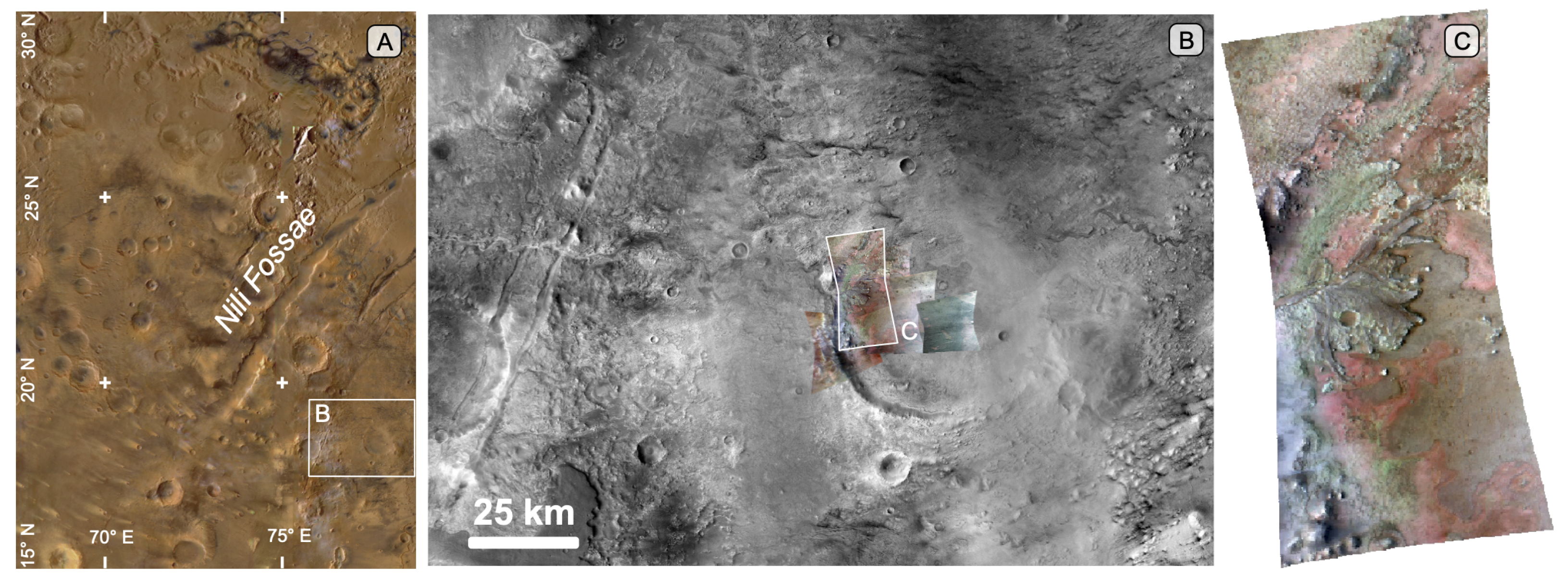
The entire Jezero area, especially the delta at its western border, has been well observed by several experiments, with a series of overlapping MRO CRISM cubes (Figure 1).
Recent detailed orbital geologic mapping of the landing site area is available [32,41], as well as geomorphologic algorithm-aided mapping [42]. Jezero Crater was selected as landing site for the Perserverance mission in 2020 [43].
Figure 1.
Location map of used cubes in the present work. (A) HRSC MC-13 quadrant color basemap [44]: of Nili Fossae and surrounding areas, including Jezero, in the highlighted subset. (B) Jezero Crater CTX mosaic [45,46] with indicated CRISM observation HRL000040FF, highlighed in white of overlapping CRISM MTRDR data covering its delta. (C) IR enhanced color composite (FAL) using as RGB R2529, R1506, R1080 [26] for CRISM observation HRL000040FF.

For reason of comparison we include datasets from the Capri Chasma area which were selected in our previous publication and summarize briefly the results in the Appendix A.
2.2. Dimensionality Reduction
In 2018, McInnes and Healy [47] presented the Uniform Manifold Approximation and Projection (UMAP) as a method for dimensionality reduction and data visualization. The idea and computation resembles the one for t-SNE [48] to a large extent. A concise overview of the algorithm is given by Allaoui et al. [49]. UMAP aims to represent the dataset X in a fuzzy topological structure. In order to build such a structure, the data points are represented in a high-dimensional weighted graph. Each edge weight depicts the probability that two points are connected and is defined by
where depicts the distance between the i-th and j-th data points, is the distance between i-th data points and its first nearest neighbor and is the scale parameter.
Subsequently, a lower-dimensional representation Y has to be determined which properly reproduces the relations of the data points in the high-dimensional graph. The projections, and , have to be mapped in the way that they correctly rebuild the similarities between the high-dimensional data points implying that the conditional probabilities and are equal. To model these low-dimensional similarities, UMAP uses a distribution similar to the Student t-distribution
In the default UMAP implementation and are used but setting and results in the Student t-distribution applied in t-SNE [47].
For optimization of the embedding Y, the low-dimensional representation UMAP uses binary cross-entropy as a cost function. It is also necessary to specify the number of nearest neighbors. As outlined by Vermeulen et al. [50], this parameter controls how UMAP handles local versus global structure in the data. A small value affects concentration on very local structure, while a larger value forces UMAP to search for larger neighborhoods.
The UMAP algorithm has achieved promising results by processing MTRDR CRISM datasets, as shown in Fernandes et al. [23]. They report superior performance of UMAP in comparison to other feature extraction techniques based on multiple scores. However, it is important to note that their work is limited to the visible and near-infrared wavelength range.
Nevertheless, we follow their parameter setup and reduce the original spectral dimension to two-dimensional data. Furthermore, we set the number of nearest neighbors to 100.
2.3. Data Pipeline
The intention of this paper is to establish a new method for spectral clustering of CRISM datasets. To include already published approaches in this research field and to exploit this existing knowledge we follow the approach of Gao et al. [11] and implement their data pipeline. This pipeline is an easy to understand procedure and consists of three main parts: preprocessing, feature extraction and clustering algorithm. Another reason for this choice is to create an equivalent basis of comparison for our new approach.
The preprocessing is an iterative process of several steps including removing nonphysical outliers and a ”per pixel” normalization. We select the same wavelength under investigation (1050 to 2550 nm) and apply also a mask to cut out the region of interest. The spectra are divided by the mean of spectra from a nearby bland area over many pixels in order to reduce systematic errors and minimize physical biases [1,51,52]. For a more detailed description, we refer to Gao et al. [11].
We extend the implementation by adding a new method for dimensionality reduction. As outlined in Section 2.2, we follow the approach of Fernandes et al. [23] and pick up the UMAP algorithm.
The autoencoder model by Gao et al. [11] is unchanged. The only modification is the insertion of the size of the latent feature space, determined by HySime [53], to a minimum value of 5.
For benchmarking the proposed techniques, we continue to use the standard statistical principal component analysis (PCA) and the t-distributed Stochastic Neighbor Embedding (t-SNE) in our data pipeline. The number of extracted principal components is also fixed at 5 as this number of components explains about 95% of the variance in the data and the increase of ratio of explained variance is very small by increasing components.
Finally, the clustering is performed by k-Means and GMM. Contrary to Gao et al. [11] we decide not to operate with a predefined number of clusters, but to explore a certain parameter space and then specify the most adequate number of clusters based on some appropriate metrics. Previous work, [11,23] suggests that a good a priori estimator is probably located between 5 and 20 clusters.
Overall, multiple different methods for generating SCMs were introduced and implemented, but we focus on the evaluation of the UMAP+k-Means approach.
2.4. Quantitative Metrics
To assess the clustering performance in a quantitative manner, we computed multiple unsupervised cluster-separation metrics for evaluation. To start with, the Calinski-Harabasz index (CH) [54] for a set of data E with pixels and split into k clusters is defined as the ratio of the dispersion between and within clusters.
where
with denoting the set of points in cluster q, the center of cluster q, the center of E and the number of points in cluster q. The measure indicates a higher score when clusters are dense and well separated.
The Davies-Bouldin index (DB) [55] is based on the average similarity between each cluster i and its most similar one j and is given by
where
is the cluster similarity measure. is the cluster diameter and is the distance between cluster centroids i and j. A lower score refers to a higher cluster validity.
As a final measure, the span of the Silhouette Coefficient (SC) is limited between −1 for incorrect clustering and +1 for highly dense clustering whereby scores around zero indicate overlapping clusters. Thus, a significant advantage of this metric is that it allows direct conclusions about the efficiency and goodness of the clustering algorithm. The SC [56] for a single sample can be written as
The measure is based on the mean distance a between a point and all other points in the same group and the mean distance b between the point and all samples in the next nearest cluster. The value of SC for a generated SCM is depicted by the average of the coefficient for each pixel.
3. Results
The presentation of results is split into two different segments. First we will report the metrics for the examined methods in order to identify the best quantitative fit for the cluster number and perform a quantitative evaluation. On the basis of these findings, we can operate with the generated SCM of the highest level of validity on the subsequent qualitative and visual analysis and have not to deal with assumptions and an arbitrary chosen number of clusters.
3.1. Quantitative Analysis
We start by calculating the metrics, introduced in Section 2.4, over the defined range of clusters. The CH and DB coefficient are fast to compute, thus they will be shown as a base line. Furthermore, these scores are used to filter the best method. As outlined by Milligan and Cooper [57], the CH score is a powerful criterion for evaluating the validity of clustering.
By inspecting the computed values we face the same issue as reported by Fernandes et al. [23] and observe also strong fluctuation in the scores. Therefore, it is difficult to draw an evidence-based conclusion about method and clusters. To treat this problem we proceed in a similar way and compute the mean over the full range of investigated clusters for each method and score. We list the results for the HRL000040FF dataset in Table 1.
According to the CH score both UMAP approaches outperform the benchmark methods and UMAP in combination with the k-Means clustering has the highest score. The PCA and autoencoder models exhibit the lowest CH value. In the case of DB, there is a similar ranking. The models using t-SNE as dimensionalirty reduction perform the best but the differences among UMAP and t-SNE are marginal. It should be emphasized again that UMAP and t-SNE are based on a related concept to cut down multidimensional data [47,48].
In order not to confine the results to a particular CRISM dataset, we include several MTRDR products in our analysis additionally. The values of both metrics for the FRT0000c564, FRT000b776 and FRT0001c71b dataset can be found in Appendix A.1. Apart from a few exceptions, there is also a consistent pattern between the CH and DB metric when establishing rank statistics of the individual scores for each dataset where a higher rank invokes denser clusters. To summarize, the UMAP+k-Means approach is able to exceed the benchmarks.
These results correspond with previous studies [23]. Fernandes et al. [23] also used the Capri Chasma set FRT0001c71b, so we confirm their findings for a different wavelength range. In summary, we provide another evidence of UMAP’s capabilities as a dimensionality reduction technique in dealing with spectral data.
So far, we examined a predefined range of possible number of clusters without knowing the ground truth labels of the pixels. In the next step, we apply the SC due to its interpretability for selecting the best convenient total number of labels. Within the scope of this examination, we restrict ourselves to the UMAP+k-Means method because of its best performance.
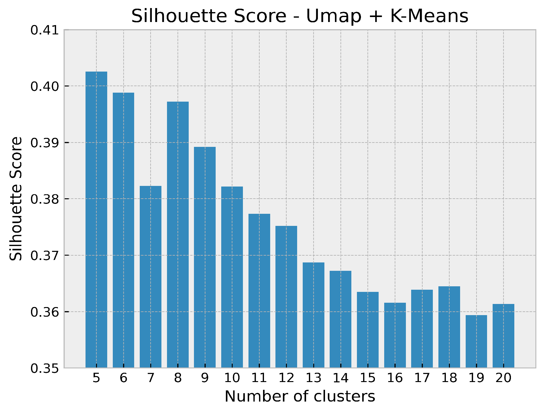
Hence, we plot the SC index against number of clusters for the Jezero Crater dataset. Apart from a little sharp bend at seven clusters Figure 2 shows an almost continuously declining graph by an increasing number of clusters. Thus, there is a strong evidence that the true number of clusters is at the lower end of the range under investigation.
In general, the values vary from below 0.36 (19 clusters) to about 0.40 (5 and 6 clusters) resulting in a moderate clustering ability for the model within this scope.
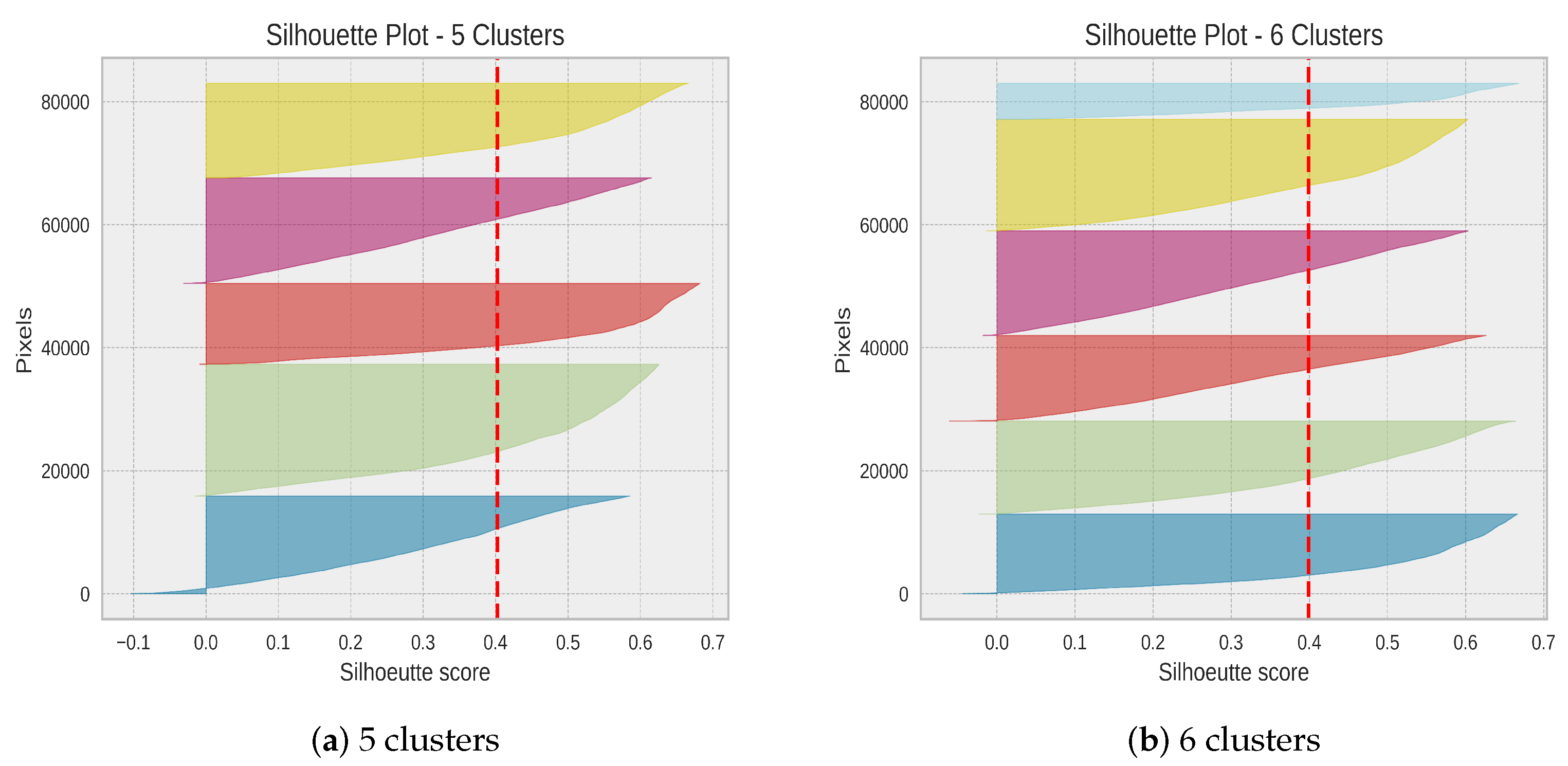
To ensure an accurate decision as possible, we illustrate the Silhouette plot for the two cluster values with the highest score in Figure 3. The Silhouette plot depicts the SC index for each single pixel grouped by class label. Moreover the dashed vertical line corresponds to the average score across all pixels. We conclude that for both numbers of classes all clusters are located above the mean score. To make a choice we have to extend the analysis.
At first, it is clearly visible that 5 clusters in Figure 3a have a more uniform thickness whereas the small class breaks this structure at 6 clusters. In spite of this fact we tend rather to 6 clusters for the following reasons: By observing the fluctuations between all clusters within one cluster environment we note a slightly higher variation for 5 clusters in comparison to 6 ones. High variation usually indicates a sub-optimal number of clusters.
Furthermore, we detect in Figure 3b several pixels with a relative negative score around 0.10. By adding one extra class this “hitch” can be rectified and the high negative scores are eliminated. Finally, we reduce the fluctuations between the clusters. Consequently, we fix this number and proceed with a UMAP+k-Means generated SCM of 6 classes.
3.2. Qualitative Analysis
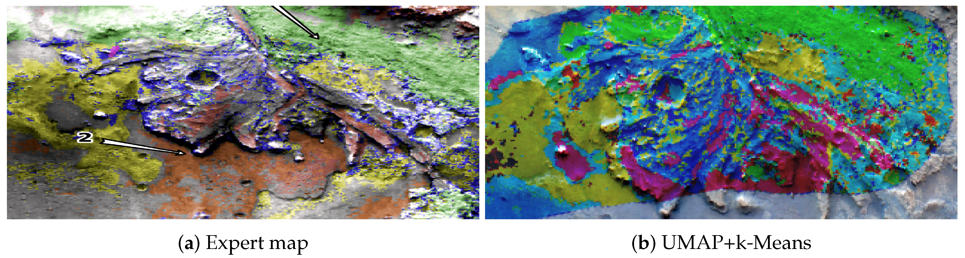
To perform qualitative evaluation we resort to the partial expert classification map used by Gao et al. [11]. This is a 6-class partially classified image of the Jezero Crater whereas five classes are directly mapped with some mineralogy and one class exists as unclassified area.
At first sight, it is evident that the expert map (Figure 4a) and the UMAP SCM (Figure 4b) exhibit strong similarity in the form and characteristics of the located clusters. The shapes of the individual clusters of both images resemble each other closely.
In order to ensure a consistent assessment, we start evaluation with the three most dominant classes: olivine, Fe/Mg smectite and carbonate; colored yellow, blue and green in expert map.
The presented SCM distinctly identifies all three regions and all areas of these classes are correctly clustered. One single difference is that, in the upper left half of expert map, the carbonate class is omnipresent while the UMAP created SCM indicates a mix of the Fe/Mg smectite and carbonate classes.
The pyroxene, orange color in Figure 4a, is likewise reliably detected by the proposed method. Besides the pyroxene deposit below the Fe/Mg smectite and partly inside this class area, it seems that the algorithm assigns some unclassified areas to pyroxene mineralogy as well.
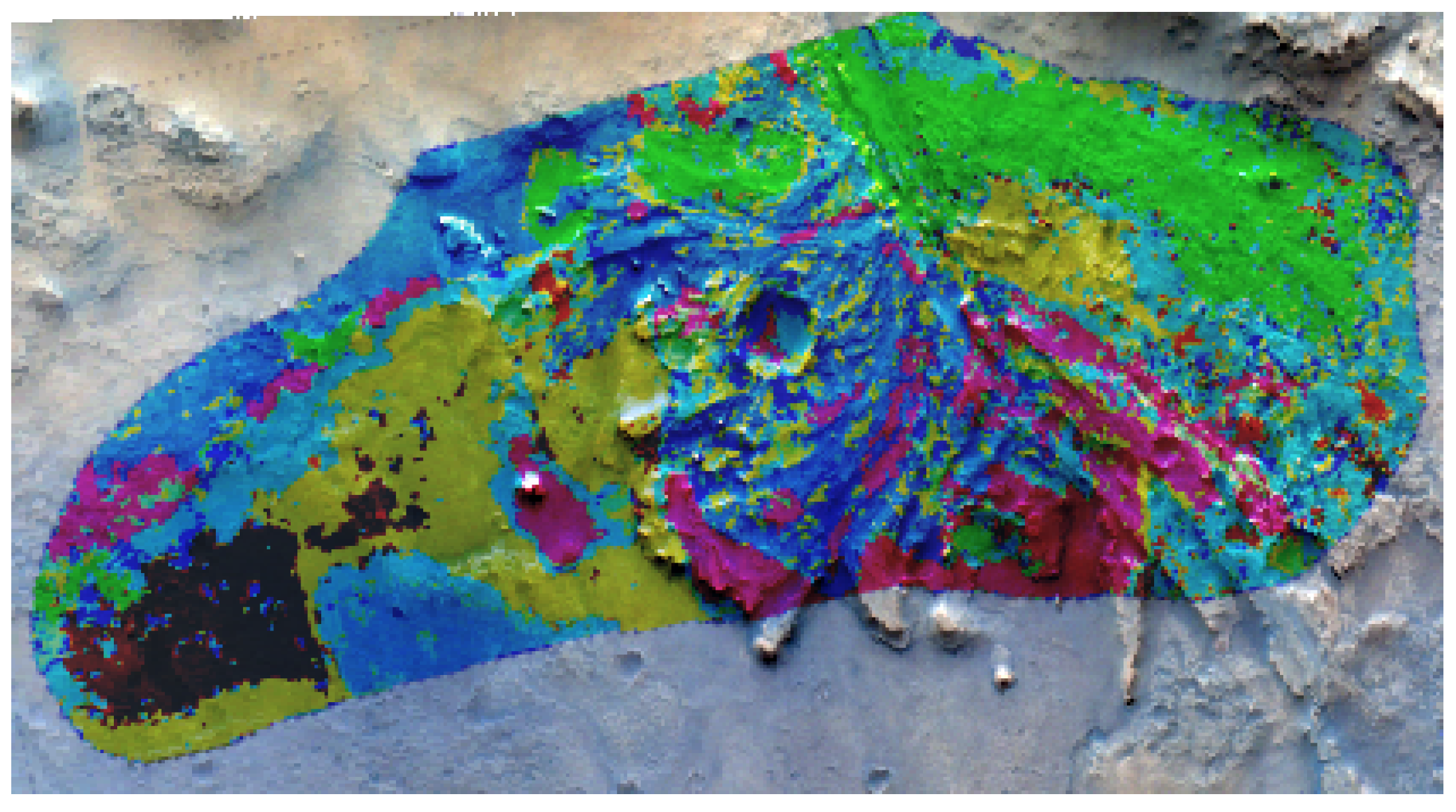
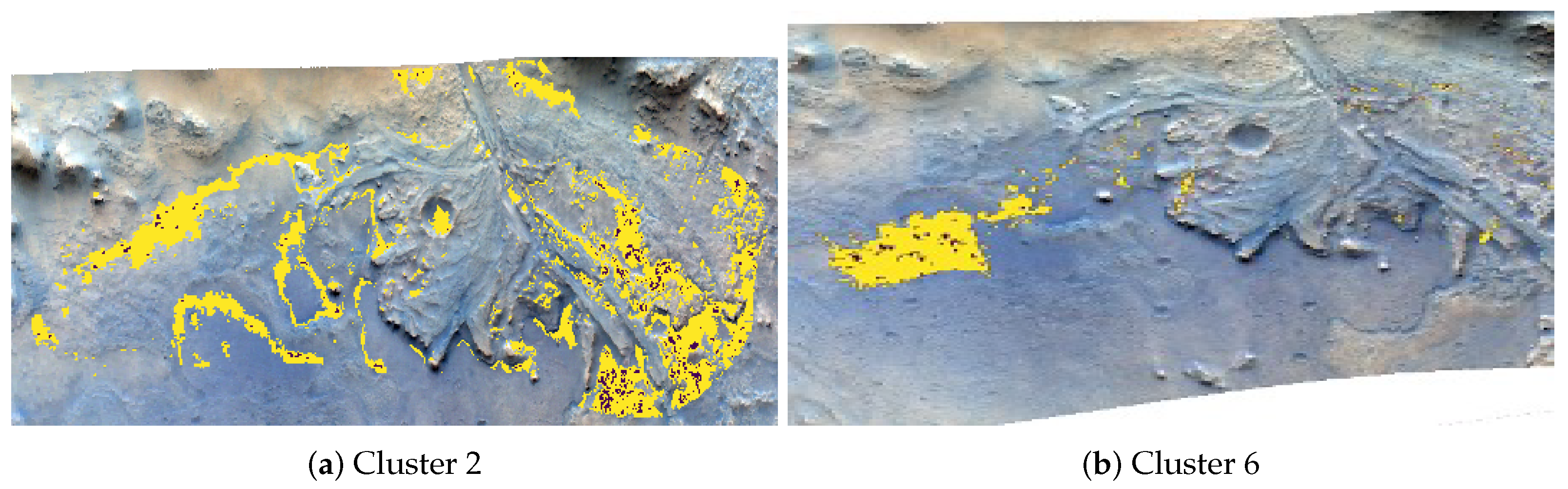
To continue with the unlabeled fraction of the expert map, we discovered a new class, including a large part of this territory. On the left side of the SCM in an area not covered by the expert map, the applied approach provides another novel group (cf. Figure 5). In order to label these areas we introduce a quantitative UMAP-based approach for automated class to mineralogy mapping in Section 4.
To complete the visual analysis we also inspect the spectra of the generated clusters since the remaining expert silica class is not seen in the produced cluster map. The correlation with the mineralogical findings is supported by calculating mean spectra per cluster.
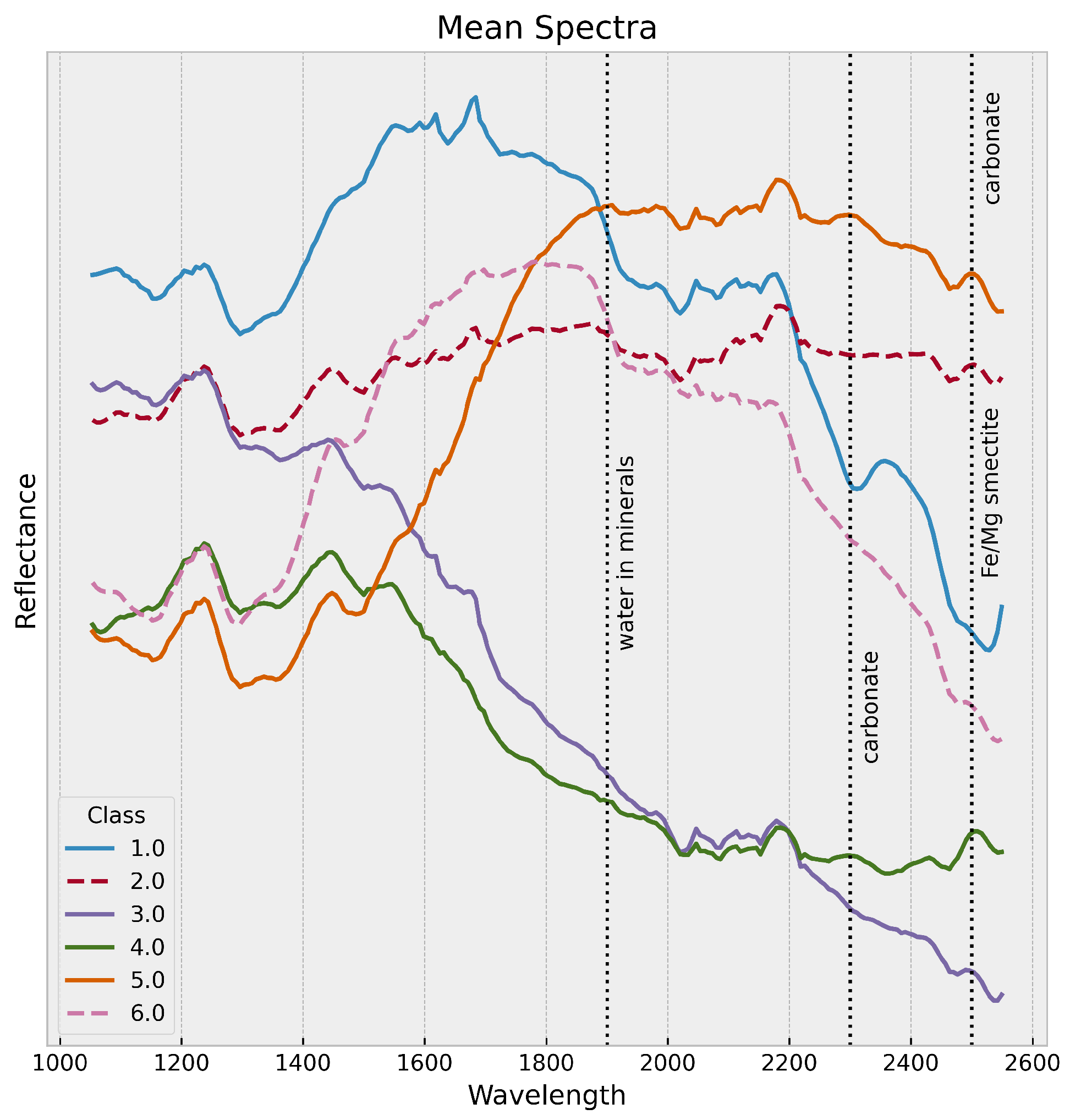
In Figure 6, we can observe the broad discriminative character of these spectra. For the dispersion of each band of the computed mean spectra for each cluster we observe values of about 5 percent. A broad absorption from 1050 nm to 1800 nm (olivine) for class 5 and a broad absorption from 1300 nm to 2300 nm (pyroxene) can be identified in case of class 4. We can see especially the key absorption of carbonates at 2500 nm (class 1). For a detailed comparison we refer to Gao et al. [11].
The benefit of using k-Means clustering is that instead of mean spectra, which are mixtures of different mineralogical fingerprints also the k-Means cluster center spectra, can be selected and analyzed, which in this case does not fundamentally differ from the mean spectra.
4. Quantitative Geological Mapping
After the visual assessment of the UMAP+k-Means spectral cluster map, we demonstrate the geological relevance of the different classes in a quantitative way. In addition, the goal is to classify mineralogically the so far unmapped area (cf. Figure 4a and Figure 5).
To connect the clusters with geo-morphological properties we use the summary products of the HRL000040FF dataset. Summary products can be applied to draw conclusions about the mineralogy and related surface types [58].
We define X as the summary products matrix with p pixels and N products. For consistency purposes we exclude several products in our investigation, mainly because the wavelength to which they respond are not within the examined range. In total, we have 29 products.
Considering a particular cluster c, where and C denotes the set of clusters, we select all pixels from X corresponding to c. Then, we pick up the first component of the UMAP feature embedding space and also mask out all unwanted pixels which are not clustered to c. Subsequent, we fit a Random Forest Regressor model M where the summary products are the input samples and the extracted latent variables of the first UMAP component are the target values y. Each forest consists of 100 trees.
After the estimator is fit, we compute permutation importance to filter the most important features G in the model. The permutation feature importance is defined to be the decline in a model score when a single feature value is randomly shuffled [59]. The idea is to establish a link between class and mineralogy based on the extracted summary products. The summarized methodology is given in Algorithm 1.
| Algorithm 1: Quantitative geological mapping |
 |
We repeated this procedure for each class c and report the results of our investigation for in Table 2. Results with fewer products are also included.
The fitted Random Forest estimators have a score of about 0.94 or higher for every c. So a high predictive power of the individual models is observable. The geology information indicated with the selected products is based on Viviano et al. [26]. All further remarks on mapping between summary products and the mineralogy refer to this work.
For all labeled classes (apart form the silica area) in expert map, the algorithm is capable of properly linking the UMAP feature embedding space to mineralogical properties. The summary browse product HCPINDEX2 is an indicator for silicate minerals and contributes significantly to the model for each cluster.
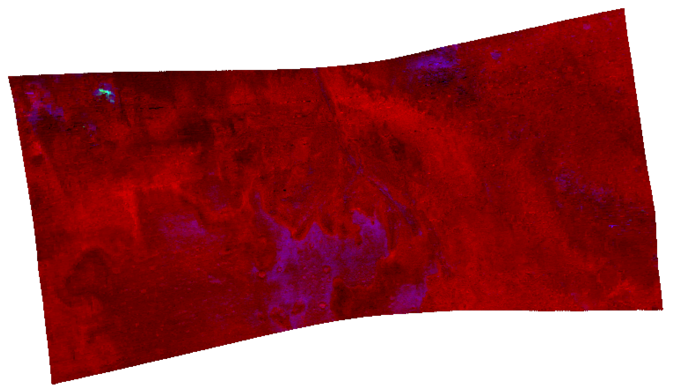
The MAF browse product (cf. Figure 7) combining OLINDEX3, LCPINDEX2 and HCPINDEX2 in its RGB channels visualizes the mafic mineralogy and highlights the presence of olivine and Fe-phyllosilicate in red.
Of particular interest are the non by expert classified regions in Figure 4a and the new clustered area on the left-side of the UMAP+k-Means SCM (cf. Figure 5). We illustrate these two classes in Figure 8. Besides the presence of HCPINDEX2, we detected the areas seen in summary product BD1750_2 and the OLINDEX3 in cluster 6. According to Viviano et al. [26] this finding indicate occurrences of aluminum clays and carbonates.This is in agreement with Horgan et al. [38], who visualized a mixture of aluminium clays and carbonates in distinct regions for Jezero crater. In general, the identified clusters characterize compositional mixtures and represent the mineralogy diversity given in [38].
5. Discussion
Based on the results of all metrics (CH and DB) the UMAP combined with the k-Means cluster procedure shows the best scores (cf. Table 1 and Appendix A.1). Consequently, this method was selected and was optimized with respect to the cluster size. The same metrics can be used and figure shows that a cluster size of 6 is proposed for the individual dataset investigated in this study.
Our analysis shows that summary browse products can be linked to each cluster in a quantitative manner. It confirms the composition given in the expert map and found by Gao et al. [11] supporting regions of carbonates, smectites and hydrated minerals. Moreover, for the 2 newly assigned clusters we could identify for cluster 1 and for cluster 6 mixtures of Al-clays and carbonates.
6. Conclusions
In this paper, a simple fast method is proposed to derive spectral clusters from hyperspectral data in the near-infrared wavelength range. The analyses show that the UMAP algorithm in combination with the k-Means clustering method, on the one hand, provides results quickly and, based on common cluster metrics, yields comparable or even better results than other proposed methods.
The evaluation of the presented cluster metrics suggests an optimal cluster number of six. The optimized cluster map for Jezero Crater shows a strong similarity to the given expert map.
Another important finding is that the method could identify two more regions, which for other methods were hard to distinguish. Spectral signatures of each cluster could clearly be related to the mineralogy (e.g., pyroxene, carbonates and Fe) found in Jezero. As the algorithm by its design executes its calculations very fast, it is useful for the evaluation and combination of large hyperspectral datasets in planetary applications.
It must be emphasized that the results can depend strongly on the data selection, the preprocessing and the signal-to-noise ratio. Thus, this procedure should rather be implemented in an iterative process with semi-manual approaches. Therefore, further iterative optimization of the procedure regarding robustness is required.
Research is still needed to quantify how the use of UMAP can address common challenges of unsupervised clustering, such as sensitivity to initial conditions, choice of parameters and data preprocessing.
To test the algorithm, we are planning an expanded analysis of the entire Jezero Crater area and to make it available to the broad community of different research groups.
Author Contributions
Writing—original draft, A.P. and M.F.; Writing—review & editing, N.T., A.P.R. and B.E. All authors contributed substantial work at every stage of this publication. All authors have read and agreed to the published version of the manuscript.
Funding
APR has been supported by the Europlanet H204 RI, and has received funding from the European Union’s Horizon 2020 research and innovation programme under grant agreement No. 871149.
Data Availability Statement
The CRISM data used here is available through the PDS Geoscience Node (https://ode.rsl.wustl.edu, accessed on 1 October 2022).
Conflicts of Interest
The authors declare no conflict of interest.
Abbreviations
The following abbreviations are commonly used in this manuscript:
| CRISM | Compact Reconnaissance Imaging Spectrometer |
| DB | Davies-Bouldin |
| GMM | Gaussian Mixture model |
| MRO | Mars Reconnaissance Orbiter |
| MTRDR | Map-projected Targeted Reduced Data Record |
| PCA | Principal omponent analysis |
| SC | Silhouette Coefficient |
| SCM | Spectral Cluster Map |
| t-SNE | t-distributed Stochastic Neighbor Embedding |
| UMAP | Uniform Manifold Approximation and Projection |
Appendix A
Appendix A.1

Table A1.
Mean of the Calinski-Harabasz and Davies-Bouldin criterion over a range of 5 to 20 clusters for the FRT0000c564 dataset, split by method. The best score for each coefficient is in bold.
Table A1.
Mean of the Calinski-Harabasz and Davies-Bouldin criterion over a range of 5 to 20 clusters for the FRT0000c564 dataset, split by method. The best score for each coefficient is in bold.
| Clustering Metrics | ||
|---|---|---|
| Methods | Calinski-Harabasz | Davies-Bouldin |
| UMAP + k-Means | 110,568 | 0.7939 |
| UMAP + GMM | 89,283 | 0.8535 |
| Autoencoder + k-Means | 28,345 | 1.2651 |
| Autoencoder + GMM | 14,133 | 2.0985 |
| PCA + k-Means | 40,415 | 1.2055 |
| PCA + GMM | 13,995 | 2.8828 |
| t-SNE + k-Means | 94,857 | 0.8092 |
| t-SNE + GMM | 88,134 | 0.8222 |
Table A2.
Mean of the Calinski-Harabasz and Davies-Bouldin criterion over a range of 5 to 20 clusters for the FRT0000b776 dataset, split by method. The best score for each coefficient is in bold.
Table A2.
Mean of the Calinski-Harabasz and Davies-Bouldin criterion over a range of 5 to 20 clusters for the FRT0000b776 dataset, split by method. The best score for each coefficient is in bold.
| Clustering Metrics | ||
|---|---|---|
| Methods | Calinski-Harabasz | Davies-Bouldin |
| UMAP + k-Means | 216,545 | 0.7192 |
| UMAP + GMM | 196,229 | 0.7545 |
| Autoencoder + k-Means | 39,897 | 1.1298 |
| Autoencoder + GMM | 16,721 | 2.1699 |
| PCA + k-Means | 59,637 | 1.3214 |
| PCA + GMM | 21,027 | 4.3664 |
| t-SNE + k-Means | 152,121 | 0.8279 |
| t-SNE + GMM | 144,334 | 0.8501 |
Table A3.
Mean of the Calinski-Harabasz and Davies-Bouldin criterion over a range of 5 to 20 clusters for the FRT0001c71b dataset, split by method. The best score for each coefficient is in bold.
Table A3.
Mean of the Calinski-Harabasz and Davies-Bouldin criterion over a range of 5 to 20 clusters for the FRT0001c71b dataset, split by method. The best score for each coefficient is in bold.
| Clustering Metrics | ||
|---|---|---|
| Methods | Calinski-Harabasz | Davies-Bouldin |
| UMAP + k-Means | 164,883 | 0.6932 |
| UMAP + GMM | 139,372 | 0.7362 |
| Autoencoder + k-Means | 31,184 | 1.0316 |
| Autoencoder + GMM | 17,879 | 1.7953 |
| PCA + k-Means | 56,562 | 0.9992 |
| PCA + GMM | 25,703 | 1.6261 |
| t-SNE + k-Means | 92,332 | 0.8048 |
| t-SNE + GMM | 86,278 | 0.8155 |
Appendix B. Citation of PDS Data Products
PDS3 data products cited in this paper as part of https://doi.org/10.17189/1519470 (accessed on 1 October 2022) have the following PDS3 DATA_SET_ID:PRODUCT_IDs:
| HRL000040FF |
| FRT0000c564 |
| FRT0000b776 |
| FRT0001c71b |
References
- Murchie, S.; Arvidson, R.; Bedini, P.; Beisser, K.; Bibring, J.P.; Bishop, J.; Boldt, J.; Cavender, P.; Choo, T.; Clancy, R.T.; et al. Compact Reconnaissance Imaging Spectrometer for Mars (CRISM) on Mars Reconnaissance Orbiter (MRO). J. Geophys. Res. Planets 2007, 112, E05S03. [Google Scholar] [CrossRef]
- Naß, A.; Di, K.; van Gasselt, S.; Hare, T.; Hargitai, H.; Karachevtseva, I.; Kersten, E.; Manaud, N.; Roatsch, T.; Rossi, A.; et al. Planetary cartography and mapping: Where we are today, and where we are heading for? Int. Arch. Photogramm. Remote Sens. Spat. Inf. Sci. 2017, 42, 105–112. [Google Scholar] [CrossRef]
- Ramsdale, J.D.; Balme, M.R.; Conway, S.J.; Gallagher, C.; van Gasselt, S.A.; Hauber, E.; Orgel, C.; Séjourné, A.; Skinner, J.A.; Costard, F.; et al. Grid-based mapping: A method for rapidly determining the spatial distributions of small features over very large areas. Planet. Space Sci. 2017, 140, 49–61. [Google Scholar] [CrossRef]
- Massironi, M.; Rossi, A.P.; Wright, J.; Zambon, F.; Poheler, C.; Giacomini, L.; Carli, C.; Ferrari, S.; Semenzato, A.; Luzzi, E.; et al. From Morpho-Stratigraphic to Geo(Spectro)-Stratigraphic Units: The PLANMAP Contribution. In Proceedings of the 2021 Annual Meeting of Planetary Geologic Mappers, Virtual, 14–15 June 2021; Volume 2610, p. 7045. Available online: https://ui.adsabs.harvard.edu/abs/2021LPICo2610.7045M (accessed on 1 October 2022).
- Semenzato, A.; Massironi, M.; Ferrari, S.; Galluzzi, V.; Rothery, D.A.; Pegg, D.L.; Pozzobon, R.; Marchi, S. An Integrated Geologic Map of the Rembrandt Basin, on Mercury, as a Starting Point for Stratigraphic Analysis. Remote Sens. 2020, 12, 3213. [Google Scholar] [CrossRef]
- Giacomini, L.; Carli, C.; Zambon, F.; Galluzzi, V.; Ferrari, S.; Massironi, M.; Altieri, F.; Ferranti, L.; Palumbo, P.; Capaccioni, F. Integration between morphological and spectral characteristics for the geological map of Kuiper quadrangle (H06). In Proceedings of the EGU General Assembly Conference Abstracts, Virtual, 19–30 April 2021; p. EGU21-15052. [Google Scholar]
- Pajola, M.; Lucchetti, A.; Semenzato, A.; Poggiali, G.; Munaretto, G.; Galluzzi, V.; Marzo, G.; Cremonese, G.; Brucato, J.; Palumbo, P.; et al. Lermontov crater on Mercury: Geology, morphology and spectral properties of the coexisting hollows and pyroclastic deposits. Planet. Space Sci. 2021, 195, 105136. [Google Scholar] [CrossRef]
- Schubert, G. Treatise on Geophysics; Elsevier: Amsterdam, The Netherlands, 2015; ISBN 978-0-444-53803-1. [Google Scholar]
- Fawdon, P.; Grindrod, P.; Orgel, C.; Sefton-Nash, E.; Adeli, S.; Balme, M.; Cremonese, G.; Davis, J.; Frigeri, A.; Hauber, E.; et al. The geography of Oxia Planum. J. Maps 2021, 17, 621–637. [Google Scholar] [CrossRef]
- Zambon, F.; Carli, C.; Wright, J.; Rothery, D.; Altieri, F.; Massironi, M.; Capaccioni, F.; Cremonese, G. Spectral units analysis of quadrangle H05-Hokusai on Mercury. J. Geophys. Res. Planets 2022, 127, e2021JE006918. [Google Scholar] [CrossRef]
- Gao, A.F.; Rasmussen, B.; Kulits, P.; Scheller, E.L.; Greenberger, R.; Ehlmann, B.L. Generalized Unsupervised Clustering of Hyperspectral Images of Geological Targets in the Near Infrared. In Proceedings of the IEEE/CVF Conference on Computer Vision and Pattern Recognition, Nashville, TN, USA, 20–25 June 2021; pp. 4294–4303. [Google Scholar]
- Timmerman, M.E. Principal Component Analysis. J. Am. Stat. Assoc. 2003, 98, 1082–1083. [Google Scholar] [CrossRef]
- Martel, E.; Lazcano, R.; López, J.; Madroñal, D.; Salvador, R.; López, S.; Juarez, E.; Guerra, R.; Sanz, C.; Sarmiento, R. Implementation of the Principal Component Analysis onto High-Performance Computer Facilities for Hyperspectral Dimensionality Reduction: Results and Comparisons. Remote Sens. 2018, 10, 864. [Google Scholar] [CrossRef]
- Rodarmel, C.; Shan, J. Principal component analysis for hyperspectral image classification. Surv. Land Inf. Sci. 2002, 62, 115–122. [Google Scholar]
- Melit Devassy, B.; George, S.; Nussbaum, P. Unsupervised Clustering of Hyperspectral Paper Data Using t-SNE. J. Imaging 2020, 6, 29. [Google Scholar] [CrossRef]
- Pouyet, E.; Rohani, N.; Katsaggelos, A.K.; Cossairt, O.; Walton, M. Innovative data reduction and visualization strategy for hyperspectral imaging datasets using t-SNE approach. Pure Appl. Chem. 2018, 90, 493–506. [Google Scholar] [CrossRef]
- Song, W.; Wang, L.; Liu, P.; Choo, K.K.R. Improved t-SNE based manifold dimensional reduction for remote sensing data processing. Multimed. Tools Appl. 2019, 78, 4311–4326. [Google Scholar] [CrossRef]
- Kohonen, T. Adaptive, associative, and self-organizing functions in neural computing. Appl. Opt. 1987, 26, 4910–4918. [Google Scholar] [CrossRef]
- Picollo, M.; Cucci, C.; Casini, A.; Stefani, L. Hyper-Spectral Imaging Technique in the Cultural Heritage Field: New Possible Scenarios. Sensors 2020, 20, 2843. [Google Scholar] [CrossRef]
- Wander, L.; Vianello, A.; Vollertsen, J.; Westad, F.; Braun, U.; Paul, A. Exploratory analysis of hyperspectral FTIR data obtained from environmental microplastics samples. Anal. Methods 2020, 12, 781–791. [Google Scholar] [CrossRef]
- Ferrer-Font, L.; Mayer, J.U.; Old, S.; Hermans, I.F.; Irish, J.; Price, K.M. High-Dimensional Data Analysis Algorithms Yield Comparable Results for Mass Cytometry and Spectral Flow Cytometry Data. Cytom. Part A 2020, 97, 824–831. [Google Scholar] [CrossRef]
- Yang, Y.; Sun, H.; Zhang, Y.; Zhang, T.; Gong, J.; Wei, Y.; Duan, Y.G.; Shu, M.; Yang, Y.; Wu, D.; et al. Dimensionality reduction by UMAP reinforces sample heterogeneity analysis in bulk transcriptomic data. Cell Rep. 2021, 36, 109442. [Google Scholar] [CrossRef]
- Fernandes, M.; Pletl, A.; Thomas, N.; Rossi, A.P.; Elser, B. Generation and Optimization of Spectral Cluster Maps to Enable Data Fusion of CaSSIS and CRISM Datasets. Remote Sens. 2022, 14, 2524. [Google Scholar] [CrossRef]
- Xia, J.; Zhang, Y.; Song, J.; Chen, Y.; Wang, Y.; Liu, S. Revisiting dimensionality reduction techniques for visual cluster analysis: An empirical study. IEEE Trans. Vis. Comput. Graph. 2021, 28, 529–539. [Google Scholar] [CrossRef]
- Pelkey, S.M.; Mustard, J.F.; Murchie, S.; Clancy, R.T.; Wolff, M.; Smith, M.; Milliken, R.; Bibring, J.P.; Gendrin, A.; Poulet, F.; et al. CRISM multispectral summary products: Parameterizing mineral diversity on Mars from reflectance. J. Geophys. Res. Planets 2007, 112, E08S14. [Google Scholar] [CrossRef]
- Viviano, C.E.; Seelos, F.P.; Murchie, S.L.; Kahn, E.G.; Seelos, K.D.; Taylor, H.W.; Taylor, K.; Ehlmann, B.L.; Wiseman, S.M.; Mustard, J.F.; et al. Revised CRISM spectral parameters and summary products based on the currently detected mineral diversity on Mars. J. Geophys. Res. Planets 2014, 119, 1403–1431. [Google Scholar] [CrossRef]
- Fassett, C.I.; Head, J.W., III. Fluvial sedimentary deposits on Mars: Ancient deltas in a crater lake in the Nili Fossae region. Geophys. Res. Lett. 2005, 32, L14201. [Google Scholar] [CrossRef]
- Schon, S.C.; Head, J.W.; Fassett, C.I. An overfilled lacustrine system and progradational delta in Jezero crater, Mars: Implications for Noachian climate. Planet. Space Sci. 2012, 67, 28–45. [Google Scholar] [CrossRef]
- Goudge, T.A.; Mohrig, D.; Cardenas, B.T.; Hughes, C.M.; Fassett, C.I. Stratigraphy and paleohydrology of delta channel deposits, Jezero crater, Mars. Icarus 2018, 301, 58–75. [Google Scholar] [CrossRef]
- Mangold, N.; Dromart, G.; Ansan, V.; Salese, F.; Kleinhans, M.G.; Massé, M.; Quantin-Nataf, C.; Stack, K.M. Fluvial regimes, morphometry, and age of Jezero crater paleolake inlet valleys and their exobiological significance for the 2020 Rover Mission Landing Site. Astrobiology 2020, 20, 994–1013. [Google Scholar] [CrossRef]
- Mangold, N.; Gupta, S.; Gasnault, O.; Dromart, G.; Tarnas, J.; Sholes, S.; Horgan, B.; Quantin-Nataf, C.; Brown, A.; Le Mouélic, S.; et al. Perseverance rover reveals an ancient delta-lake system and flood deposits at Jezero crater, Mars. Science 2021, 374, 711–717. [Google Scholar] [CrossRef]
- Stack, K.M.; Williams, N.R.; Calef, F.; Sun, V.Z.; Williford, K.H.; Farley, K.A.; Eide, S.; Flannery, D.; Hughes, C.; Jacob, S.R.; et al. Photogeologic map of the perseverance rover field site in Jezero Crater constructed by the Mars 2020 Science Team. Space Sci. Rev. 2020, 216, 127. [Google Scholar] [CrossRef]
- Morgan, A.M.; Wilson, S.A.; Howard, A.D. The global distribution and morphologic characteristics of fan-shaped sedimentary landforms on Mars. Icarus 2022, 385, 115137. [Google Scholar] [CrossRef]
- Weitz, C.M.; Bishop, J.L.; Grant, J.A.; Wilson, S.A.; Irwin, R.P., III; Saranathan, A.M.; Itoh, Y.; Parente, M. Clay sediments derived from fluvial activity in and around Ladon basin, Mars. Icarus 2022, 384, 115090. [Google Scholar] [CrossRef]
- Ehlmann, B.L.; Mustard, J.F.; Fassett, C.I.; Schon, S.C.; Head, J.W., III; Des Marais, D.J.; Grant, J.A.; Murchie, S.L. Clay minerals in delta deposits and organic preservation potential on Mars. Nat. Geosci. 2008, 1, 355–358. [Google Scholar] [CrossRef]
- Ehlmann, B.L.; Mustard, J.F.; Swayze, G.A.; Clark, R.N.; Bishop, J.L.; Poulet, F.; Des Marais, D.J.; Roach, L.H.; Milliken, R.E.; Wray, J.J.; et al. Identification of hydrated silicate minerals on Mars using MRO-CRISM: Geologic context near Nili Fossae and implications for aqueous alteration. J. Geophys. Res. Planets 2009, 114, E00D08. [Google Scholar] [CrossRef]
- Goudge, T.A.; Mustard, J.F.; Head, J.W.; Fassett, C.I.; Wiseman, S.M. Assessing the mineralogy of the watershed and fan deposits of the Jezero crater paleolake system, Mars. J. Geophys. Res. Planets 2015, 120, 775–808. [Google Scholar] [CrossRef]
- Horgan, B.H.; Anderson, R.B.; Dromart, G.; Amador, E.S.; Rice, M.S. The mineral diversity of Jezero crater: Evidence for possible lacustrine carbonates on Mars. Icarus 2020, 339, 113526. [Google Scholar] [CrossRef]
- Brown, A.J.; Viviano, C.E.; Goudge, T.A. Olivine-carbonate mineralogy of the Jezero crater region. J. Geophys. Res. Planets 2020, 125, e2019JE006011. [Google Scholar] [CrossRef]
- Tarnas, J.; Stack, K.; Parente, M.; Koeppel, A.; Mustard, J.; Moore, K.; Horgan, B.; Seelos, F.; Cloutis, E.; Kelemen, P.B.; et al. Characteristics, Origins, and Biosignature Preservation Potential of Carbonate-Bearing Rocks Within and Outside of Jezero Crater. J. Geophys. Res. Planets 2021, 126, e2021JE006898. [Google Scholar] [CrossRef]
- Sun, V.Z.; Stack, K.M. Geologic Map of Jezero Crater and the Nili Planum Region, Mars; US Geological Survey Scientific Investigations Map; US Department of the Interior, US Geological Survey: Reston, VA, USA, 2020; Volume 3464.
- Wright, J.; Barrett, A.M.; Fawdon, P.; Favaro, E.A.; Balme, M.R.; Woods, M.J.; Karachalios, S. Jezero crater, Mars: Application of the deep learning NOAH-H terrain classification system. J. Maps 2022, 18, 484–496. [Google Scholar] [CrossRef]
- Bell, J.F.I.; Maki, J.N.; Alwmark, S.; Ehlmann, B.L.; Fagents, S.A.; Grotzinger, J.P.; Gupta, S.; Hayes, A.; Herkenhoff, K.E.; Horgan, B.H.N.; et al. Geological, multispectral, and meteorological imaging results from the Mars 2020 Perseverance rover in Jezero crater. Sci. Adv. 2022, 8, eabo4856. [Google Scholar] [CrossRef]
- Gwinner, K.; Jaumann, R.; Hauber, E.; Hoffmann, H.; Heipke, C.; Oberst, J.; Neukum, G.; Ansan, V.; Bostelmann, J.; Dumke, A.; et al. The High Resolution Stereo Camera (HRSC) of Mars Express and its approach to science analysis and mapping for Mars and its satellites. Planet. Space Sci. 2016, 126, 93–138. [Google Scholar] [CrossRef]
- Malin, M.C.; Bell, J.F., III; Cantor, B.A.; Caplinger, M.A.; Calvin, W.M.; Clancy, R.T.; Edgett, K.S.; Edwards, L.; Haberle, R.M.; James, P.B.; et al. Context camera investigation on board the Mars Reconnaissance Orbiter. J. Geophys. Res. Planets 2007, 112, E05S04. [Google Scholar] [CrossRef]
- Dickson, J.; Kerber, L.; Fassett, C.; Ehlmann, B. A global, blended CTX mosaic of Mars with vectorized seam mapping: A new mosaicking pipeline using principles of non-destructive image editing. In Proceedings of the Lunar and Planetary Science Conference, The Woodlands, TX, USA, 19–23 March 2018; Lunar and Planetary Institute: The Woodlands, TX, USA, 2018; Volume 49, pp. 1–2. [Google Scholar]
- McInnes, L.; Healy, J.; Melville, J. UMAP: Uniform Manifold Approximation and Projection for Dimension Reduction. arXiv 2018. [Google Scholar] [CrossRef]
- Van der Maaten, L.; Hinton, G. Visualizing data using t-SNE. J. Mach. Learn. Res. 2008, 9, 2579–2625. [Google Scholar]
- Allaoui, M.; Kherfi, M.L.; Cheriet, A. Considerably Improving Clustering Algorithms Using UMAP Dimensionality Reduction Technique: A Comparative Study. In Proceedings of the Image and Signal Processing, Marrakesh, Morocco, 4–6 June 2020; El Moataz, A., Mammass, D., Mansouri, A., Nouboud, F., Eds.; Springer International Publishing: Cham, Switzerland, 2020; pp. 317–325. [Google Scholar]
- Vermeulen, M.; Smith, K.; Eremin, K.; Rayner, G.; Walton, M. Application of Uniform Manifold Approximation and Projection (UMAP) in spectral imaging of artworks. Spectrochim. Acta Part A Mol. Biomol. Spectrosc. 2021, 252, 119547. [Google Scholar] [CrossRef] [PubMed]
- Weitz, C.M.; Bishop, J.L. Stratigraphy and formation of clays, sulfates, and hydrated silica within a depression in Coprates Catena, Mars. J. Geophys. Res. Planets 2016, 121, 805–835. [Google Scholar] [CrossRef]
- Murchie, S.L.; Seelos, F.P.; Hash, C.D.; Humm, D.C.; Malaret, E.; McGovern, J.A.; Choo, T.H.; Seelos, K.D.; Buczkowski, D.L.; Morgan, M.F.; et al. Compact Reconnaissance Imaging Spectrometer for Mars investigation and data set from the Mars Reconnaissance Orbiter’s primary science phase. J. Geophys. Res. Planets 2009, 114, E00D07. [Google Scholar] [CrossRef]
- Bioucas-Dias, J.M.; Nascimento, J.M.P. Hyperspectral Subspace Identification. IEEE Trans. Geosci. Remote Sens. 2008, 46, 2435–2445. [Google Scholar] [CrossRef]
- Caliński, T.; Harabasz, J. A dendrite method for cluster analysis. Commun. Stat.-Theory Methods 1974, 3, 1–27. [Google Scholar] [CrossRef]
- Davies, D.L.; Bouldin, D.W. A Cluster Separation Measure. IEEE Trans. Pattern Anal. Mach. Intell. 1979, PAMI-1, 224–227. [Google Scholar] [CrossRef]
- Rousseeuw, P.J. Silhouettes: A graphical aid to the interpretation and validation of cluster analysis. J. Comput. Appl. Math. 1987, 20, 53–65. [Google Scholar] [CrossRef]
- Milligan, G.W.; Cooper, M.C. An examination of procedures for determining the number of clusters in a data set. Psychometrika 1985, 50, 159–179. [Google Scholar] [CrossRef]
- Kamps, O.; Hewson, R.; van Ruitenbeek, F.; van der Meer, F. Defining surface types of Mars using global CRISM summary product maps. J. Geophys. Res. Planets 2020, 125, e2019JE006337. [Google Scholar] [CrossRef]
- Breiman, L. Random Forests. Mach. Learn. 2001, 45, 5–32. [Google Scholar] [CrossRef] [Green Version]
Figure 2.
Silhouette Score of UMAP+k-Means as a function of the number of clusters for HRL000040FF dataset.
Figure 2.
Silhouette Score of UMAP+k-Means as a function of the number of clusters for HRL000040FF dataset.

Figure 3.
Silhouette Plot UMAP+k-Means for 5 and 6 clusters and the HRL000040FF set.

Figure 4.
On the left side, the expert map used by Gao et al. [11] is presented. Each class is associated with a different color. In total, 6 classes are clustered as follows: olivine, yellow; pyroxene, orange; carbonate, green; Fe/Mg smectite, blue; silica, magenta and unclassified area, gray. On the right side, the UMAP+k-Means generated spectral cluster map with 6 identified clusters is illustrated. The same detail, as captured by expert map (a), is shown.

Figure 5.
Spectral cluster map by UMAP-k-Means and 6 clusters for the complete clustered area of Jezero Crater.
Figure 5.
Spectral cluster map by UMAP-k-Means and 6 clusters for the complete clustered area of Jezero Crater.

Figure 6.
Mean spectra per cluster as representative fingerprint. Key unique absorptions at 1900 nm (water in minerals), 2300 nm and 2500 nm (carbonate) and 2300 nm (Fe/Mg smectite) are marked with vertical dotted lines.
Figure 6.
Mean spectra per cluster as representative fingerprint. Key unique absorptions at 1900 nm (water in minerals), 2300 nm and 2500 nm (carbonate) and 2300 nm (Fe/Mg smectite) are marked with vertical dotted lines.

Figure 7.
The MAF browse product of the MTRDR product HRL000040FF. This image browse product shows information related to mafic mineralogy and denotes olivine and Fe-phyllosilicate in red color [26].
Figure 7.
The MAF browse product of the MTRDR product HRL000040FF. This image browse product shows information related to mafic mineralogy and denotes olivine and Fe-phyllosilicate in red color [26].

Figure 8.
The two novel classes identified by the UMAP+k-Means and pictured as an overlay of the true image of Jezero Crater. Left: cluster 2 embraces mainly the unclassified area of expert map (cf. Figure 4a). Right: cluster 6 indicates a new mineralogy class.
Figure 8.
The two novel classes identified by the UMAP+k-Means and pictured as an overlay of the true image of Jezero Crater. Left: cluster 2 embraces mainly the unclassified area of expert map (cf. Figure 4a). Right: cluster 6 indicates a new mineralogy class.

Table 1.
Mean of the Calinski-Harabasz and Davies-Bouldin criterion over a range of 5 to 20 clusters for the HRL000040FF dataset, split by method. The best score for each coefficient is in bold.
Table 1.
Mean of the Calinski-Harabasz and Davies-Bouldin criterion over a range of 5 to 20 clusters for the HRL000040FF dataset, split by method. The best score for each coefficient is in bold.
| Clustering Metrics | ||
|---|---|---|
| Methods | Calinski-Harabasz | Davies-Bouldin |
| UMAP + k-Means | 114,928 | 0.8179 |
| UMAP + GMM | 109,469 | 0.8349 |
| Autoencoder + k-Means | 25,649 | 1.2435 |
| Autoencoder + GMM | 12,648 | 2.5199 |
| PCA + k-Means | 53,478 | 1.0643 |
| PCA + GMM | 19,594 | 2.6050 |
| t-SNE + k-Means | 78,578 | 0.8072 |
| t-SNE + GMM | 75,248 | 0.8120 |
Table 2.
Quantitative geological mapping of the six identified regions for the Jezero Crater (HRL000040FF). The products conforming to the expert map (cf. Figure 4a) are in bold, according to Viviano et al. [26].
| Cluster | Selected Products | Geology | Expert Map |
|---|---|---|---|
| 1 | HCPINDEX2, CINDEX2, BD1750_2, | Carbonates | Carbonates |
| 2 | BD1750_2, HCPINDEX2 | Gypsum, Alunite | unclassified |
| 3 | CINDEX2, RPEAK1 | Fe, Fe-Carbonate | Fe |
| 4 | D2300, HCPINDEX2 | Pyroxene, Silicates | Pyroxene |
| 5 | HCPINDEX2, RPEAK1 | Fe-mineralogy (suggest Olivine) | Olivine |
| 6 | BD1750_2, OLINDEX3, HCPINDEX2 | Gypsum, Alunite, Olivine | unclassified |
Disclaimer/Publisher’s Note: The statements, opinions and data contained in all publications are solely those of the individual author(s) and contributor(s) and not of MDPI and/or the editor(s). MDPI and/or the editor(s) disclaim responsibility for any injury to people or property resulting from any ideas, methods, instructions or products referred to in the content. |
© 2023 by the authors. Licensee MDPI, Basel, Switzerland. This article is an open access article distributed under the terms and conditions of the Creative Commons Attribution (CC BY) license (https://creativecommons.org/licenses/by/4.0/).
Share and Cite
MDPI and ACS Style
Pletl, A.; Fernandes, M.; Thomas, N.; Rossi, A.P.; Elser, B. Spectral Clustering of CRISM Datasets in Jezero Crater Using UMAP and k-Means. Remote Sens. 2023, 15, 939. https://doi.org/10.3390/rs15040939
AMA Style
Pletl A, Fernandes M, Thomas N, Rossi AP, Elser B. Spectral Clustering of CRISM Datasets in Jezero Crater Using UMAP and k-Means. Remote Sensing. 2023; 15(4):939. https://doi.org/10.3390/rs15040939
Chicago/Turabian StylePletl, Alexander, Michael Fernandes, Nicolas Thomas, Angelo Pio Rossi, and Benedikt Elser. 2023. "Spectral Clustering of CRISM Datasets in Jezero Crater Using UMAP and k-Means" Remote Sensing 15, no. 4: 939. https://doi.org/10.3390/rs15040939
Note that from the first issue of 2016, this journal uses article numbers instead of page numbers. See further details here.