Learning from the past: reservoir computing using delayed variables
 Ulrich Parlitz1,2*
- 1Biomedical Physics Group, Max Planck Institute for Dynamics and Self-Organization, Göttingen, Germany
- 2Institute for the Dynamics of Complex Systems, Georg-August-Universität Göttingen, Göttingen, Germany
Reservoir computing is a machine learning method that is closely linked to dynamical systems theory. This connection is highlighted in a brief introduction to the general concept of reservoir computing. We then address a recently suggested approach to improve the performance of reservoir systems by incorporating past values of the input signal or of the reservoir state variables into the readout used to forecast the input or cross-predict other variables of interest. The efficiency of this extension is illustrated by a minimal example in which a three-dimensional reservoir system based on the Lorenz-63 model is used to predict the variables of a chaotic Rössler system.
1 Introduction
Machine learning methods are becoming increasingly important in science and in everyday life, and new approaches and concepts are being developed all the time. One method for predicting temporal developments that was already proposed at the beginning of the millennium is reservoir computing. In this approach, a reservoir of dynamic elements, often consisting of a recurrent neural network, is driven by a (known) input signal, and the dynamic response of the reservoir system is used to predict the future evolution of the input signal or other relevant quantities, e.g., by the linear superposition of its state variables. This basic concept was developed1 and publicized independently by Jaeger [4] and Maass et al. [5] in 2001 and 2002, respectively, and represents a special form of random projection networks [6]. Jaeger introduced the so-called echo state networks, i.e., recurrent neural networks whose nodes consist of one-dimensional dynamic elements with a sigmoid activation function. The reservoir system presented by Maass et al. consisted of a neural system with spike dynamics and was called liquid state machine [5, 7]. Only later did the generic term reservoir computing become established for the entire class of machine learning methods that exploit the dynamic response of a driven dynamical system for prediction and classification of input signals [8].
Reservoir computing differs from most other machine learning methods by the nature of the training, which here essentially consists of solving a linear system of equations to determine the weights of the linear superposition of (functions of) the reservoir variables [9]. However, this fast learning step usually has to be repeated several times in order to optimize the hyperparameters of the reservoir system, i.e., the parameters that control its dynamical features. Nevertheless, the overall training of a reservoir system is generally faster than, for example, that of a deep neural network. However, as Jaeger pointed out in his foreword to the book Reservoir Computing: Theory, Physical Implementations, and Applications by Nakajima and Fischer [10], a deeper understanding of reservoir computing is still lacking despite extensive research since its invention.
Over the past 20 years, not only has the methodology of reservoir computing been researched and improved, but practical applications have also been proposed, including, for example, speech recognition [11], detection of epileptic seizures [12], control methods [13], online prediction of movement data [14], approximation of Koopman operators [15], or diverse approaches for signal classification [16–26], including data structure prior to extreme events [27] and reservoir time series analysis to distinguish different signals [28].
In order to achieve fast and energy-efficient performance, hardware implementations of reservoir systems have been devised, opening a new field called physical reservoir computing [29], often based on optical systems [e.g., [30–33]] and other hardware platforms [26, 34–37]. A readable introduction to reservoir computation in general and physical reservoir computing in particular can be found in the review article by Cucchi et al. [38]. For more details and examples, the book by Nakajima and Fischer [10] is another excellent source.
While reservoir computing has been extensively studied in the machine learning community since the seminal works of Jaeger and Maass et al., it initially received little attention in the field of non-linear dynamics, with a few exceptions [39–41]. This changed in the last 7 years, mainly due to the work of Ott and collaborators [42–45]. The main reasons for this are the generally increasing interest in machine learning methods and applications, as well as the fact that reservoir computing is a very interesting and not yet fully explored dynamic process.
A key feature of suitable reservoir systems is their ability to generate a unique response for a given input time series, independent from the reservoir system's initial conditions. In the context of reservoir computing, this feature is called echo state property or fading memory. If the known input signal itself originates from a dynamical system, this system and the reservoir system form a pair of uni-directionally coupled (sub-) systems where generalized synchronization can occur. Generalized synchronization is a necessary condition for reproducible response and thus for the functionality of the reservoir system and closely related to the echo state property. The aim of this article is therefore to look at reservoir computing from a non-linear dynamics perspective in order to deepen the understanding of how it works and to provide a review of recently proposed extensions using delayed variables. To this end, in Sections 2.1–2.3, we first formulate the concept of reservoir computing in general terms, i.e., not limited to the use of recurrent neural networks as reservoir systems. In Section 2.4, the echo state property and its relation to generalized synchronization will be discussed. The classical examples of general-purpose reservoir systems are echo state networks, which are introduced in Section 2.5. In Section 3.1, we present an extension of the output function by adding input and state variables from the past. This promising approach is illustrated in Sections 3.2–3.5 using a minimal reservoir system consisting of a single three-dimensional system based on the Lorenz-63 differential equations, which is used to predict the variables of a chaotic Rössler system. Some other concepts to improve the performance of reservoir computing will be briefly discussed in Section 4.
2 Fundamentals of reservoir computing
2.1 Continuous and discrete reservoir systems
In reservoir computing, an input signal drives a dynamical system, the reservoir, and the state variables of this system (evolving in time) are used for generating some desired output, like a temporal forecast of the input signal or a cross-prediction of some other signal that is assumed to be related to the input signal.
The concept of reservoir computing can be implemented and studied in continuous or discrete time. The discrete time framework is used, for example, if a time series sampled in time is input of a dynamical system simulated on a digital computer (e.g., a recurrent network). With discrete time, the reservoir system reads2
where is the state of the reservoir system and the input time series, that is often given by sampling a time continuous signal u[n] = u(nTsmp) where Tsmp denotes the sampling time.
If reservoir computing is implemented on an analog computer or using any driven real-world (physical, biological, etc.) system, a formal description using continuous time systems [i.e., ordinary differential equations (ODEs)] is in general more appropriate. If the input is given by Nin signals in time, the reservoir system reads
where is the state of the reservoir system and Nres its dimension.
The output of the reservoir system is given by a parameterized readout function g(u, r) of the reservoir state r and the input u.3
During training (or learning), the parameters of g are the only quantities to be estimated and adapted. Since the functional form of the function g should enable efficient training, functions that are linear in their parameters are preferred for reservoir computing design, such as linear superpositions of Kj basis functions to define the component vj of the output v as
where the coefficients wkj constitute the parameters to be estimated using training data (see Section 2.3). The basis functions can be any linear or non-linear function [e.g., polynomials [43] and radial basis functions [46]], but in most applications affine linear or quadratic polynomials have been used as readout functions of reservoir systems. Affine linear output functions
are given by an Nesv = 1 + Nin + Nres dimensional extended state vector and an Nesv×Nout output matrix Wout whose elements are the parameters to be estimated during training [here (·;·;·) denotes concatenation and x is a row vector]. Equation (4) provides the Nout dimensional output signal (or time series) v where the j-th column of Wout contains superposition coefficients wkj for computing the element vj of the row vector v and the number of basis functions Kj equals Nesv for all j = 1, …, Nout components of the output v.
In general, the number of basis functions Kj can be different for each component vj and can be larger than the dimension Nesv of the extended state vector x, for example, if (additional) non-linear basis functions like polynomials [43] or radial basis functions are used. Such non-linear output functions not only extend the possibilities of approximating complicated functional relations, but can also be used to break unwanted symmetries of the reservoir system [47].
In this and the following sections, the reservoir systems are assumed to be finite dimensional. However, also dynamical systems with an infinite dimensional state space, like delay differential equations or extended systems described by partial differential equations may act as dynamical reservoirs. For example, reservoir computing using feedback loops (e.g., ring lasers) has been demonstrated experimentally and in numerical simulations. The dynamics of these delay-based reservoir systems4 is governed by delay differential equations5 ṙ(t) = f(r(t), r(t−τ), u(t)) where τ equals the time delay due to the internal feedback loop (round-trip time of the light in case of a ring laser, for example). The output is obtained by sampling the solution r(tn) at discrete times along the delay line. For a more detailed description of this type of delay-based reservoir computing, see the pioneering work of Appeltant et al. [30, 48], a recent review by Chembo [49], references [31, 32, 50, 51] for implementations and extensions, and Hülser et al. [52] for a detailed discussion of the influence of (multiple) delay times as successfully used by Stelzer et al. [53]. We will not go further into delay-based reservoir computing, but most of the aspects and features discussed below also apply to this approach.
2.2 Forecasting, cross-prediction, and classification
Reservoir computing can be used for essentially all machine learning tasks including:
(i) forecasting a future value u(t + Tprd) of the input signal u(t) (in the case of discrete systems: u[n]↦u[n + Nprd]),
(ii) cross-predicting another variable y(t) or its future value y(t + Tprd), or
(iii) classifying the input by some constant label.
In all these cases, the reservoir system is trained such that it provides a task-dependent target value (the training is described in more detail in Section 2.3). Tasks (i) and (ii) can also be combined to learn and provide a signal, which is then used to control another dynamical process. Using different readout functions, a single reservoir system can perform different tasks like (i), (ii), and (iii) in parallel.
There are two main options for predicting the evolution of a target value over time: (a) performing the desired prediction in a single step or (b) decomposing the prediction interval into many small steps, resulting in an iterated prediction for discrete systems and an autonomous ODE in the case of a continuous reservoir system. Both approaches are now described in more detail.
2.2.1 Single-step prediction
With single-step prediction, the reservoir system is trained such that its output v(t) provides (an estimate of) the desired future value u(t + Tprd) or y(t + Tprd) (analogously for discrete systems predicting Nprd steps ahead). With this method, the reservoir system continuously generates forecasts of the variables of interest that may be used, for example, in control loops (to compensate latency) or for early warning of upcoming (extreme) events. This approach will be illustrated in Section 3.2. The larger the prediction time Tprd, however, the more complicated is the function to be approximated (in particular for signals from chaotic systems). Therefore, an iterated prediction with a sequence of smaller time steps is often more advantageous [54, 55] as will be discussed in the next section.
2.2.2 Output feedback and iterated prediction
Let us first consider the case of a discrete reservoir system where the output v[n] is a function g(r[n]) = (1;r[n])Wout of the state of the reservoir system r[n], only, and provides an estimate of the next future value of the input u[n + 1], which is then used as input for the next prediction step. With this feedback, the reservoir system becomes an autonomous system6
and after Nprd iteration steps, the desired prediction of u[n + Nprd] is obtained. If the output of the reservoir system is y≠u, then the input u[n + 1] for the next temporal iteration step has to be reconstructed from y[n + 1] to close the feedback loop, e.g., with the help of another reservoir system trained for cross-prediction y↦u. In general, however, for predicting another target variable, y[n + Nprd]), in some applications, one would first use iterated prediction to estimate u[n + Nprd] and then use the same7 or another reservoir system to cross-predict y[n + Nprd]) from u[n + Nprd].
Feedback can also be used to predict the future evolution of the input u(t + Tprd) using a continuous reservoir system (Equation 2). In this case, the output v(t) = g(r(t)) = (1;r(t))Wout of the reservoir system is trained to approximate the input u(t), and the result is substituted in Equation (2) for u(t). The resulting autonomous reservoir system
is integrated up to time t + Tprd to obtain u(t + Tprd) ≈ v(t + Tprd). Of course, if the input signal originates from a chaotic system and if the reservoir system has learned this dynamics, sensitive dependence on initial conditions will lead to predictions that deviate exponentially from the true input signal as Tprd increases, i.e., only short- or medium-term forecasts are possible. This prediction horizon is often compared with the Lyapunov time, which is the inverse of the largest Lyapunov exponent of the dynamical system that generated the input signal. Similar to synchronization with sporadic coupling [56, 57], a divergence of the prediction from the true time evolution can be avoided by feeding the given input signal u into the autonomous reservoir system from time to time [58].
2.2.3 Short-term prediction and climate
Since training optimizes only the performance of short-term predictions, when applied for many steps, iterated prediction not only deviates from the true evolution of the target signal but may also result in asymptotic behavior with dynamical and statistical properties that are (very) different from the target signal (e.g., periodic or diverging solutions, instead of chaos; different values of characteristics like fractal dimensions or Lyapunov exponents). Such long-term features (corresponding to ergodic properties) are also referred to as climate [42, 59], and it depends on the application whether it is more important to optimize the accuracy of the short- or medium-term predictions, or whether a correct representation of the climate is the main goal [44, 60–62].
Using input data from different sources (e.g., different chaotic attractors), a reservoir system with feedback can be trained to produce forecasts and the climates of these sources [63–65]. In this case, the autonomous reservoir system is trained to have coexisting attractors and multifunctionality to predict input signals from different sources, and it is possible to switch between the coexisting attractors using suitable input signals [63].
2.3 Training of the reservoir system
The only parameters to be determined during training are the elements of the output matrix Wout. If the output function g is chosen to be linear in these parameters, training consists essentially in solving a linear set of equations as will be shown in the following. First, a training set {(v[m], y[m])} consisting of m = 1, …, M sampled output values v[m] and target values has to be generated, where v[m] = v(mTsmp) and y[m] = y(mTsmp) in the case of a continuous reservoir system sampled with a sampling time Tsmp. To make sure that the dynamical evolution of the reservoir system is (asymptotically) independent from its (in general unknown) initial conditions, this sampling has to be preceded by a sufficiently long transient (or washout) time Ttrs = MtrsTsmp of Mtrs time steps, a requirement that will be discussed in more detail in Section 2.4.
The output of the reservoir system matches the target if Wout can be chosen such that the linear equation
holds, where X is an M × Nesv matrix whose rows are extended states x[m] and Y is an M × Nout matrix whose rows are the corresponding target values y[m]. If M > Nesv, this linear set of equations has more equations (M·Nout) than unknowns (Nesv·Nout), while for M < Nesv, it is underdetermined. In the latter case, regularization is required to avoid solutions Wout with very large matrix elements, but also for the over-determined case M > Nesv, the solution may suffer from instabilities in the case that some columns of X are almost collinear, i.e., that elements of u and/or r are highly correlated. This problem can be addressed by means of Tikhonov regularization (also known as Ridge Regression) where a cost function
with
is minimized that contains a regularization term punishing too large matrix elements . The regularization parameter β>0 controls the impact of the regularization and has to be chosen suitably. The minimum of this cost function (Equation 8) is given by
where XT denotes the transposed of X. Alternatively, the solution Wout (Equation 9) minimizing the cost function (Equation 8) can be computed using the singular value decomposition (SVD) of X = USVT, where S is a diagonal matrix with Sij ≥ 0 for i = j and Sij = 0 for i ≠ j. In this case, the minimum of the cost function (Equation 8) is given by
with
Instead of Tikhonov regularization, one can also use the Moore-Penrose-pseudo inverse X + of X, such that
Using the SVD of X = USVT, the pseudo-inverse X + can be written as X + = VEUT with
where ϵ>0 represents the numerical resolution but can also be chosen larger and then serves as a regularization parameter.8 The difference between the definitions of the matrices D and E is illustrated in Figure 1. In both cases, the impact of very small or vanishing singular values Sii is limited by bounding their inverse values 1/Sii (see Equations 10 and 11). For sufficiently long training data, i.e., with M > Nesv, the pseudo-inverse based on Equation (11) may provide better results than Tikhonov regularization (Equation 10), because the latter has a stronger bias for small but not too small singular values.
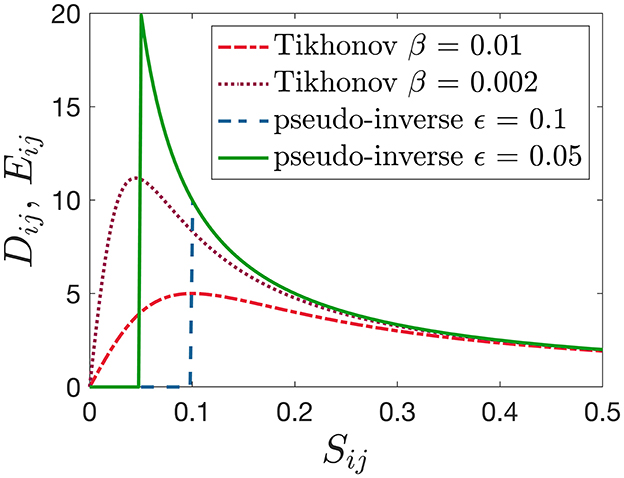
Figure 1. Graphical illustration of the inversion of the SVD matrix S using Tikhonov regularization (Equation 10) or when computing the pseudo-inverse (Equation 11) for different values of the regularization parameters β and ϵ, respectively.
An alternative to minimizing the quadratic cost function (Equation 8) is L1-optimization, where the Euclidean norm ∥·∥2 is replaced by the L1-norm ∥·∥1, and the solution of the minimum of the resulting cost function can be computed using the Lasso algorithm [66–68]. In this case, the computation of the optimal coefficients is more time consuming, but since many of them are zero after training, the calculation of the readout consists of fewer operations and is therefore more efficient.
An important feature of a trained reservoir system is its capability for generalization on similar but previously unseen data. This is notoriously difficult to determine in advance, but for reservoir systems consisting of (a certain class of) recurrent neural networks, Han et al. [69] derived a bound for the generalization error.
2.4 Echo state property and generalized synchronization
To use a trained reservoir system in any application, e.g., prediction, its output has to be reproducible and unique if the same input signal is presented again, independently from the (often unknown) initial state of the reservoir at the beginning. In reservoir computing, this feature is known as echo state property (ESP) or fading memory, and it is formally defined as follows [4, 70, 71].
For all input sequences from a compact set U and any pair of initial conditions of the reservoir system, r[0] and , the iterated application of Equation (1) results in (or correspondingly for continuous time systems (Equation 2) with input signal u(t)).
If the reservoir system fulfills this criterion, it asymptotically “forgets” its initial state after some transient or washout time Ttrs, and its (current) state is given by a so-called echo state function ξ of the semi-infinite input sequence r[n] = ξ(…, u[n−1], u[n]) [4].
If the input signal was generated by a dynamical system or z[n + 1] = fsrc(z[n]), this system and the reservoir system can be seen as a pair of uni-directionally coupled dynamical systems (i.e., a drive-response configuration), where the echo state property occurs due to generalized synchronization [72–80]. With generalized synchronization, the state of the driven system, i.e., the reservoir, r(t) is (asymptotically) a function ψ(z(t)) of the state z(t) of the driving system generating the input signal, i.e., (or for discrete systems). In this way, each state variable ri(t) of the reservoir system represents after a sufficiently long (synchronization) transient time Ttrs, a dynamically emerging function ψi(z) of the state of the driving system that is used in the output Equation (4) as a non-linear basis function for approximating the target v [39]. This function ψi(z) corresponds to the echo state function r[n] = ξ(…, u[n−1], u[n]), if the input u is generated by the dynamical system and given by an observation function u = h(z). In this case, (previous) values of the input time series are given by functions of the current state z[n] of the driving system, because u[n−k] = h(z[n−k]) = h(ϕ−k(z[n])), where ϕ−k denotes the inverse flow of the driving system. The same holds for continuous reservoir systems driven by an input signal from a continuous dynamical system.
So in principle, any driven dynamical system may be used as a reservoir system if it exhibits generalized synchronization with the dynamical system generating the input signal. This includes analog computers or even real physical processes. The occurrence of generalized synchronization can by checked, for example, using conditional Lyapunov exponents or the auxiliary system approach [74, 76, 79]. However, generalized synchronization is only a necessary condition for fulfilling the echo state property but is not sufficient to guarantee the same unique response for all initial conditions of the reservoir system. There may be different coexisting attractors that lead to different reproducible asymptotic responses depending on the initial conditions of the driven system. This form of multistability has to be taken in to account [63–65] or excluded to guarantee a unique response and thus the echo state property.
The emerging functions ψi are continuous, and their smoothness properties depend on the (transversal) contraction properties of the response system. In general, the stronger this contraction, i.e., the faster two neighboring trajectories r(t) and converge with , the smoother are the functions ψi. A mathematically more rigorous treatment of this feature can be found, for example, in a series of publications by Stark et al. on forced dynamical systems [81–83]. A detailed mathematical analysis of the differentiability properties of the echo state functions and their importance for successful reservoir computing was carried out by Grigoryeva and Ortega [84]. Hart et al. [85] proved under some mild assumption that ψ almot surely provides an embedding of the dynamics of the driving system into the state space of the reservoir system, and that there exists a linear readout function φ(r) that predicts arbitrarily well the input values provided that the dimension of the reservoir system is high enough. If this prediction is used to substitute the input u of the reservoir system an autonomous system r[n + 1] = f(r[n], φ(r[n])) or is obtained (see Section 2.2.2). A well-trained autonomous reservoir system reproduces the Lyapunov exponents of the driving system, i.e., the Lypunov exponents of the input signal are a subset of the Lyapunov exponents of the autonomous reservoir [42]. In this context, Platt et al. [86] found that the prediction time for autonomous reservoir systems with a low Kaplan–Yorke dimension is the longest. Carroll [87] obtained a similar result for the Kaplan–Yorke dimension calculated from the full Lyapunov spectrum of the coupled drive-response system.
If the response system exhibits no contraction, generalized synchronization and the echo state property cannot occur. If, on the other hand, contraction is too strong, the emerging functions ψi are very (too) smooth and, therefore, not very well-suited to be used for approximating functional relations of target signals y, whose dependence on the state z is given by a less smooth and more complicated function. It is therefore important that the contraction properties of the response system can be adapted to generate the appropriate level of smoothness of the output for a given modeling task. In case of echo state networks (see Section 2.5), contraction is controlled by the spectral radius of the reservoir matrix Wres, and in many studies, it has been observed that weak contraction provides best performance of the reservoir system. Weak contractions lead to long synchronization transients, and an increased memory capacity of the reservoir system quantified by the ability to recover past input signals u[n−k] from the current state r[n] of the reservoir system [88]. A comprehensive discussion of the role of generalized synchronization and the question under which conditions iterated prediction of a reservoir reproduces the attractor (i.e., the climate) of the driving system was given by Lu et al. [44]. Mathematical criteria and statements for the latter can also be found in [85].
Dambre et al. [89] pointed out that the information processing capacity of a driven dynamical system with fading memory (i.e., echo state property) and linear readout is bounded by the number of linearly independent functions of the input the system can compute (or generate). In general, good performance of any reservoir system can be expected if the time series ri[n] given by the state variables of the reservoir system are linearly independent, because in this case the dimension of the linear subspace spanned by the columns of the matrix X is large. This feature can be quantified by the rank of the covariance matrix XTX, also called covariance rank [90–93]. A large covariance rank will not guarantee good performance, but in general, a reservoir with a large rank will be superior to a reservoir generating output with a lower covariance rank.
An extension of generalized synchronization is consistency [94], which quantifies the degree of functional dependency of a driven dynamical system on its input in terms of the linear correlation of the reservoir variables when repeatedly driven by the same input. If the echo property is fulfilled, the consistency is equal to one. Consistency has also been used for studying reservoir computing, in particular with experimental set-ups [31, 32]. Lymburn et al. [95] found that even in cases of non-complete consistency, such inconsistent echo state networks may exhibit very good performance because there are subspaces in the state space of the reservoir system that represent signals with high consistency. This observation may lead to an enhanced understanding of the computational capacity of chaotic or noisy response systems and novel unsupervised optimization procedures. Extending the basic concept of consistency, Jüngling et al. [96] have developed an approach to investigate the propagation and distribution of information-carrying signals in a reservoir system.
Last but not least, reservoir computing using echo state networks has also been used to approximate the emergent functions that arise from the generalized synchronization of different coupled systems [97].
2.5 Echo state networks
An echo state network [4, 98] is a recurrent neural network acting as a dynamical reservoir that can be given by a set of ordinary differential equations (ODEs)
or a set of updating rules for echo state networks that operate in discrete time
In both cases, q(·) denotes an activation function (applied component-wise), which in most applications is a sigmoid function like q(·) = tanh(·). is a vector of different bias constants bi∈ℝ affecting the dynamics of the state variable ri of the i-th node of the network and may be used to break the symmetry of the dynamical equations [47]. The constants γ > 0 and α ≥ 0 are called leaking rates and can be used to adjust the temporal scale of the echo state network to that of the input signal and also to control the (fading) memory of the network dynamics. The parameter σ > 0 controls the amplitude of the input signal. Both matrices, Win and Wres, are chosen randomly. Since the impact of the input can be controlled by the parameter σ, the elements of the input matrix Win can, for example, be uniformly distributed in the interval [−1, 1]. The internal coupling matrix of the reservoir Wres and the leaking rates γ or α have to be chosen in a way that the echo state network possesses the echo state property [99].
Furthermore, in many cases, sparse coupling matrices Wres provided better performance. Therefore, a sparseness parameter δ is introduced quantifying the relative number of non-zero elements of Wres. With a sparse coupling topology, the echo state network decomposes into many loosely coupled subsystems, and this may result in a more diverse dynamics of its nodes [100].
All network parameters mentioned so far, Nres, Wres, Win, b, σ, γ, α, δ, and the regularization weight β, are hyperparameters, which have to be chosen by the user when designing the echo state network and may have a major impact on its performance. Optimal values of hyperparameters can be found by grid search or using gradient methods [70, 101] or Bayesian optimization [102]. Improved predictive performance and enhanced generalization capabilities have been obtained with first projecting the state of the reservoir system to a lower dimensional space before computing the parameters of the readout function [103]. An approach for reducing the size of the network using proper orthogonal decomposition (or principle component analysis) of its internal dynamics was suggested by Jordanou et al. [104].
An important feature of reservoir systems is their memory capacity, i.e., their ability to reconstruct and output previous input signals from the past. The memory capacity of an echo state network increases with the network size and is also affected by the other hyperparameters [detailed studies using i.i.d. random input time series can, for example, be found in [88, 105, 106]]. For a given input signal and task, there is an optimal amount of memory of the reservoir system maximizing its performance, but it is difficult to determine it in advance without simulating the full reservoir computer [107].
Reservoir systems do not have to be non-linear, because linear system may also generated non-linear output due to their exponential solution functions [108]. Bollt [109] showed that an echo state function with a linear activation function is equivalent to a vector autoregressive (VAR) model and if a quadratic readout function is used this is equivalent to non-linear VAR (NVAR) models. Furthermore, he showed that linear echo state networks are less effective but in combination with quadratic readout prediction results for chaotic time series may be acceptable. Carroll and Pecora also found that linear node dynamics in echo state networks is less effective [90]. In their study of the impact of network structure, they considered the rank of the covariance matrix of the output, symmetries, and the resulting memory capacity and found that sparsity of the internal coupling matrix is beneficial, but much more important for improving the performance may be flipped links in the network. To cope with dynamics on multiple time scales, Tanaka et al. [110] considered echo state networks with heterogeneous leaky integrator (LI) neurons, where the parameter α in Equation (12) is chosen different for each node.
The performance of echo state networks (and reservoir computing in general) also depends on the available input u, more precisely whether full or only partial information about the state of the driving system is provided (e.g., a single component of the state vector of the dynamical system generating the data). Storm at al. [92] demonstrated that if only partial information is available, the reservoir system needs some memory to generated implicitly a delay embedding. This is not necessary if the full state is presented as input, and in this case, even an echo state network without internal dynamics can provide good predictions [62], because static non-linear maps of the input state (given by the activation functions) are sufficient. However, Lymburn et al. [97] have shown that the inclusion of internal dynamics can still be advantageous compared with memoryless reservoir computing, even if the complete state is available as input, if the input–output function to be learned is itself dynamically generated and has a very complex (e.g., fractal) form.
Gauthier et al. [111] compared echo state networks with NVAR modeling using polynomial basis functions and found that these types of NVAR models provide similar or even better predictions, while requiring shorter time series for training and less computational resources.9 Jaurigue and Lüdge [115] discussed this approach in the context of other machine learning methods including delay-based reservoir computing with multiple delay loops [53]. An evaluation of the performance of different echo state networks with different network structures compared with other machine learning methods was presented by Shahi et al. [116]. They found that reservoir computing and NVAR models achieve similar prediction results.
3 Reservoir computing using delayed variables
3.1 Extending the set of basis functions
The performance of a reservoir computing system can be improved by increasing its state-space dimension Nres, which results in a larger number of basis function ψi used for generating the output (Equation 4) [89]. This increases, however, the computational load for simulating the reservoir system. An alternative is the use of delayed input and state variables, u(t − τu) and r(t − τr), respectively, because they provide additional basis functions. Let ϕt be the flow of the driving dynamical systems such that , and let the input signal of the reservoir system be given by u(t) = h(z(t)) where h denotes the observation function. In this case, after the synchronization transient (washout time) decayed, delayed input and reservoir state variables can be (asymptotically) written as functions of the state z(t) of the driving system at time t
Here, the functions and , represented by u(t−τu) and r(t−τr), respectively, can be used to extend the set of basis functions entering in the computation (Equation 4) of the output of the reservoir system.10
The extension of reservoir computing using past states of the reservoir system has been first studied by Marquez et al. [117], Sakemi et al. [118], and Del Frate et al. [119] who all found significant improvement in the performance of the reservoir system, a result that will be confirmed in the following. Later, Carroll and Hart [91] showed for an opto-electronic delay-based reservoir computer with only a small number of virtual nodes that time-shifted readout increases the rank and memory of the reservoir computer. In general, using many different delay times τu and τr increases the number of columns of the matrix X and (if suitable) its covariance rank, which leads to an improved performance of the reservoir [91, 93].
Duan et al. [120] showed that linear readout functions including delayed variables may also provide an embedding of the input dynamics, and they discuss the trade-off between the number of delays and the state space dimension of the reservoir system (i.e., the number of nodes in case of a recurrent network).
Jaurigue et al. [121] showed that the performance of an unoptimized reservoir system can significantly be improved by adding a time-delayed input signal. In their study, they simulated time multiplexed delay-based reservoir computing with a single non-linear element that can be implemented using optical hardware. In a recent study, Jaurigue and Lüdge [122] showed that the dependance of reservoir performance on the choice of suitable hyperparameter values can be reduced by including delayed variables.
3.2 Predicting Rössler dynamics using a Lorenz-63 based reservoir system
To demonstrate the effectiveness of reservoir computing using delayed variables, we will consider now a very simple example: a three-dimensional reservoir system based on the Lorenz-63 system [79, 123]
This system fulfills the echo state property for all initial conditions r(0) (see Appendix).
The parameter μ is used to adapt the time scale to that of the driving signal u(t) and controls the transversal contraction properties of the response system (see Appendix). Therefore, it is a hyperparameter that has to be carefully chosen.
Using an affine linear readout function, the output component vj (j = 1, 2, 3) sampled at times tn = nTsmp is given by
or using the notation vj[n] = vj(tn)
The minimal reservoir system (Equation 15) will be used to predict the variables zi of a chaotic Rössler system [79, 124]
from the observations u[m] = u(tm) = z1(tm) of the first variable at times tm = mTsmp, where Tsmp denotes the sampling time.
3.3 Cross-prediction of unobserved state variables of the Rössler system
In our first example, the reservoir system (Equation 15) is used to cross-predict the variables z2(tm) and z3(tm) of the chaotic Rössler system (Equation 17) from previous observations u[k] = u(tk) = z1(tk) of the first variable z1 with k ≤ m. This task is known in control theory as state observer. If a training time series u(tk) of length M is available,11 the computation of the weights wij in Equation (16) consists of solving the set of linear equations (Equation 7) with
where
and
with the columns of Y given by the target values zi[m] = zi(tm) of the Rössler system.12 This set of linear equations (Equation 18) is solved for the weights Wout = X + Y using the Moore-Penrose pseudo-inverse X + of X (see Section 2.3) with , where σ1 denotes the largest singular value of X.
Figure 2 shows predictions of z2 and z3 obtained with a training time series of length M = 50, 000 and sampling time Tsmp = 0.01 corresponding to a time interval of length 500. While the cross-prediction of the z2 component may be acceptable, the peaks of the z3 variable are not correctly reconstructed. This relatively poor result should be expected given the fact that only time series of u, r1, r2, and r3 have been used to predict the target signal. The bottom panels of Figures 2C, F show the dependence of the Normalized Root Mean Squares Error (NRMSE) of the test data
on the parameter μ for both target signals y2 and y3, respectively. Here, ȳj stands for the mean value of yj, represents its variance, and Ntest is the length of the time series used to compute the test error. The NRMSE quantifies the performance of the reservoir compared with a prediction of yj by its mean value ȳj. The lowest errors occur for predictions of z2 at μ = 0.025 and for z3 near μ = 1.1. This large difference in optimal μ values may be due to different smoothness properties of the functions ψi required to successfully predict z2 or z3 (see Section 2.4 and Appendix). Such differences with respect to optimal (hyper) parameters may complicate the simultaneous prediction of different target variables using output from the same reservoir system.
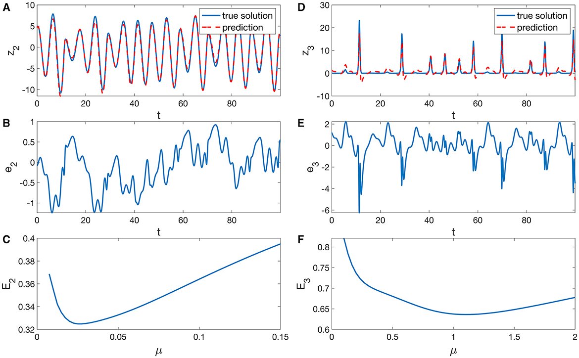
Figure 2. Cross-prediction of the (A) z2(t) and (D) z3(t) variables of the chaotic Rössler system (Equation 17) from u = z1 using the Lorenz-63 based reservoir system (Equation 15). The elements of the output matrix Wout were computed using Equations (18) and (11) with regularization parameter , where σ1 denotes the largest singular value of X. The diagrams (B, E) show the corresponding prediction errors ej(t) = vj(t) − zj(t). In (C, F), the dependences of the test errors E2 and E3 (Equation 19) on the reservoir parameter μ are shown. The examples (A, B, D, E) have been computed for μ = 0.025 and μ = 1.1, respectively, which are close to the minima of the test errors shown in (C, F).
3.4 Cross-prediction using delayed variables
We will now increase the pool of signals (or basis functions) using past values of the input signal (Equation 13) and the state variables (Equation 14) of the reservoir system (Equation 15) in terms of delay vectors u(t) = [u(t − Nuτu), …, u(t − τu), u(t)] and rk(t) = [rk(t − Nrτr), …, rk(t − τr), rk(t)], which can for t = mTsmp, τu = LuTsmp and τr = LrTsmp be written as13
To simplify the presentation, we use the same number of Nu = Nr = Ndelay delayed variables u and r in the following. Using the row vectors u[m] and rk[m], the linear set of equations for computing the parameters of the affine linear output function reads
with K = 1 + 4(Ndelay + 1) = 5 + 4Ndelay basis functions. This set of linear equations can again be solved using the pseudo-inverse of X or any other method for solving a linear set of equations using regularization (see Section 2.3). Note that with delay M + Ndelay samples at times t1−Ndelay, …, t1, …, tM−1, tM are required for constructing the matrix X and that the number of basis functions K = 5 + 4Ndelay used for approximating the target function increases linearly with Ndelay. Furthermore, the rows of matrix X represent a projection of the state (z, r) of the full coupled system to a K-dimensional space (providing an embedding if K is large enough).
Figure 3 shows prediction results for z2 and z3 obtained with Ndelay = 100 and delay times (τu = 0.32, τr = 0.37) for z2 and (τu = 0.03, τr = 0.30) for z3, such that the delay vectors for z2 cover approximately a period of time of 32 < Ndelayτu, r < 37 corresponding to about six oscillations of z1 and z2. As can be seen, not only the z2-component of the Rössler system is recovered with high precision, but also the peak structure of the input signal and the z3-component.
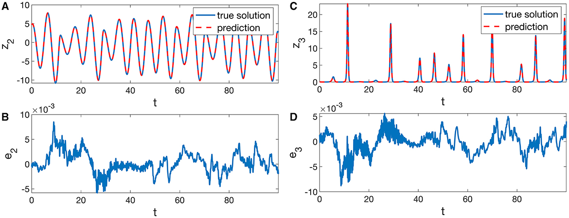
Figure 3. Cross-prediction of the (A) z2 and (C) z3 variables of a chaotic Rössler system (Equation 17) from its first variable z1 using a Lorenz-63 based system (Equation 15) with delayed readout (Equations 20 and 21). Hyperparameters for the prediction of z2 are μ = 0.81, τu = 0.32, τr = 0.37, Ndelay = 100 and for the prediction of z3 the values μ = 0.83, τu = 0.03, τr = 0.30, Ndelay = 100 were used. The elements of the output matrix Wout were computed using Equations (22) and (11) with regularization parameter , where σ1 denotes the largest singular value of X. The diagrams (B, D) show the corresponding prediction errors ej(t) = vj(t) − zj. The mean test errors (Equation 19) equal E2 = 0.0203 and E3 = 0.0274.
The delay times τu, τr and the number of delays Nu and Nr are additional hyperparameters that have to be carefully chosen for a given prediction problem. One method for optimization is the maximization of the rank correlation [93], which can also be achieved by a targeted use of the zeros or minima of the autocorrelation functions of the input signal and the reservoir states.
3.5 Predicting future evolution
So far, only the current values of the target signals z2(t) and z3(t) have been reconstructed using input signals z1(t) until time t. As discussed in Section 2.2, reservoir systems can also be used for predicting the future evolution of the variables of interest. Figure 4 shows prediction results where the output of the reservoir system provides the target signals z2(t + Tprd) and z3(t + Tprd) for a prediction time of Tprd = 10 (in units of the time variable of the Rössler system). As indicated by the green horizontal bars in Figures 4A, C, this period of time corresponds to about 1.6 oscillation periods of the z2 variable. The continuously available future values of the target signals can be used, for example, for implementing a control system or for predicting the occurrence of “extreme events” like the peaks of the z3 variable.
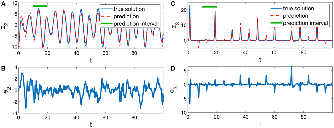
Figure 4. Prediction of future values of the (A) z2 and (C) z3 variables of a chaotic Rössler system (Equation 17) from its first variable z1 using a Lorenz-63-based system (Equation 15) with delayed readout (Equations 20 and 21). The prediction time interval Tprd = 10 is indicated by a horizontal bar. Hyperparameters for the prediction of z2 are μ = 3.76 τr = 0.15, τu = 0.24 Ndelay = 100, and for the prediction of z3, the values μ = 3.6 τr = 0.22, τu = 0.18, Ndelay = 100 were used. The values of the output matrix Wout were computed using Equations (22) and (11) with regularization parameter , where σ1 denotes the largest singular value of X. The diagrams (B, D) show the corresponding prediction errors. The mean test errors (Equation 19) equal E2 = 0.443 and E3 = 0.539.
A prediction scheme based on delayed variables can also be implemented using feedback (see Section 2.2.2). In this case, the output which is fed back as input to the reservoir is a function of delayed state variables v(t) = g(r(t), r(t−τ1), r(t−τ2), ….), and the resulting autonomous reservoir system is given by a delay differential equation with multiple delays.
4 Extensions and improvements to reservoir computing
The use of delayed variables is not the only way to extend and improve the reservoir computing paradigm. Many studies for echo state networks have been performed to learn more about criteria for choosing the most suitable network architecture [125–129] and alternative activation functions (e.g., relu, radial basis functions, ….). Shahi et al. [130] reported more robust and accurate predictions when reservoir computing is combined with an autoencoder, where an echo state network operates in the latent space of the autoencoder. Nathe et al. [131] investigated the effects of measurement noise and found that the performance of reservoir observers can be significantly improved with low-pass filtering applied to the input signal.
Another extension is knowledge-based reservoir computing [132, 133], where valuable information from existing models based on first principles and/or other empirical models are combined with a reservoir system. Existing models may be incomplete and are thus quantitatively not exact, but they still contain the knowledge of the field and provide at least a good first guess for the desired output. In this case, machine learning methods like reservoir computing can be used to add required corrections to the predicted values or to create the conditions under which the model can be applied. For example, to make use of existing knowledge-based dynamical models like ordinary or partial differential equations, one has to know suitable initial conditions, e.g., the full state of a dynamical system, which is in most cases not given by the data available. In this case, a reservoir system (like the example presented in Section 3.3) can be used to reconstruct the full state vector from available observations, which can then be used as initial condition of the mathematical model to compute its future evolution. Such hybrid configurations are called knowledge-based or physics-informed14 machine learning and often require (much) less training data compared with purely data-driven algorithms (i.e., without employing a physics-based model). A comparison of different approaches for hybrid reservoir computing was recently provided by Duncan and Räth [134]. If no model based on first principles is available, one can also combine reservoir computing with another type of data-driven model [e.g., some ODE model obtained by sparse identification of a polynomial vector field [135]].
Reservoir computing has also been successfully applied to spatially extended systems by using several echo state networks operating in parallel to avoid the use of extremely large networks [45, 86, 136–138]. Last but not least, it should be mentioned that the concept of reservoir computing can also be used with quantum systems. Such quantum reservoir computing is currently a very active field [139–142], but beyond the scope of this review.
5 Conclusion
Reservoir computing is an efficient method for time series prediction and has mainly been studied using recurrent networks called echo state networks. However, in principle, any driven dynamical system may serve as a reservoir of output signals that can be used, for example, to predict or classify the input signal if the system has a fading memory of its own initial condition. This feature is also called echo state property, and it is closely linked to generalized synchronization. The concept of reservoir computing can be implemented not only on digital computers but also on a hardware basis. Such physical reservoir computing systems may offer advantages like very high speed or low energy consumption.
Recently, it has been shown that the inclusion of past values of input and reservoir state variables in the readout function can significantly improve the performance of reservoir computing. In particular, for echo state networks, it has been shown that this type of extended readout may be used to reduce the number of nodes (i.e., the size of the network) required to achieve a given level of predictive power [117–120]. As this is a simple but very effective method for improving reservoir computing, this approach has been dealt with in more detail in this overview. We demonstrated and confirmed its effectiveness using a minimal three-dimensional reservoir system based on the Lorenz-63 system. Using delayed variables, this low-dimensional reservoir system can reconstruct all state variables of a chaotic Rössler system from an univariate time series of the first Rössler variable and even provide some medium-time prediction of their future evolution. This example was not only chosen to demonstrate the effectiveness of using delayed variables but also to show that there alternative reservoir systems and that it is not mandatory to use high-dimensional systems such as large networks. Of course, a reservoir system with only three variables cannot compete in performance with high-dimensional systems such as echo state networks with hundreds or thousands of nodes. But it may serve, for example, as a building block of an approach with several similar systems running in parallel. This can be done in continuous time, as here, but also using low-dimensional discrete dynamical systems. Such structures may lead to novel reservoir system designs that can be efficiently implemented in (physical or biological) hardware.
Author contributions
UP devised the manuscript, generated all figures, and wrote the text.
Funding
The author acknowledges support by the Max Planck Society (MPG).
Acknowledgments
The author would like to thank Stefan Luther, Luk Fleddermann, Hiromichi Suetani, and all members of the Biomedical Physics Research Group at the Max Planck Institute for Dynamics and Self-Organization for their support and stimulating scientific discussions.
Conflict of interest
The author declares that the research was conducted in the absence of any commercial or financial relationships that could be construed as a potential conflict of interest.
Publisher's note
All claims expressed in this article are solely those of the authors and do not necessarily represent those of their affiliated organizations, or those of the publisher, the editors and the reviewers. Any product that may be evaluated in this article, or claim that may be made by its manufacturer, is not guaranteed or endorsed by the publisher.
Footnotes
1. ^The basic idea of reservoir computing was already described in publications by Kirby [1], Schomaker [2], and Dominey [3] before the work of Jaeger and Maass et al. appeared.
2. ^Sometimes, u[n] is used instead of u[n + 1] to define a discrete reservoir system r[n + 1] = f(r[n], u[n])). However, the definition (Equation 1) is better suited to include in the output Equations (3) and (4) the most current information at time n, which is given by r[n] and u[n].
3. ^Depending on the application of the reservoir system, the output may be defined as a function of the reservoir state r, only. This is often the case, for example, when implementing autonomous reservoir systems whose output signal is fed back into their input, see Section 2.2.2.
4. ^The term delay-based reservoir system is used if the internal dynamics of the reservoir system contains time delays. This is to be distinguished from the use of delayed variables in the output function, which is the main topic of the current review, see Section 3.
5. ^Delay-based reservoir systems are often described by a single variable r.
6. ^A reservoir system driven by an input signal (Equations 1 or 2) is sometimes called a listening reservoir and autonomous reservoir systems with a feedback loop (Equations 5 and 6) are referred to as predicting reservoirs.
7. ^The same reservoir can, e.g., be trained to model the function u[n−1]↦y[n] by determining a suitable output matrix Wout.
8. ^Many programming languages such as Matlab, Julia, or Python provide a function pinv(A, tol) for computing the pseudo-inverse of a matrix A with an optional parameter tol corresponding to ϵ.
9. ^In [111], the NVAR approach presented is called “next-generation reservoir computing”, a title that is possibly ironic but slightly misleading, since static functions are used for prediction and not the response of a dynamical system. Modeling and approximating the flow in embedding space using static non-linear functions goes back to the 1980s using polynomial [112] or radial basis functions [54], including Tikhonov regularization [113]. In this context, early work on NARMAX models should also be mentioned, see, for example, [114].
10. ^Note that here multiple delays are used in the readout function, only. This is different from delay-based reservoir computing using (multiple) delays mentioned in Section 2.1.
11. ^Here, we assume that prior to the sampling of the training data a sufficiently long transient time Ttrs has elapsed.
12. ^Since the target signal y1 = u = z1 is known, only the outputs v2 and v3 have to be computed to estimate the unobserved variables z2 = y2 and z3 = y3 for reconstructing the state z of the Rössler system.
13. ^In general, different numbers of delay terms with different delay times could be used for u and each variable rk. This would, however, increase the number of hyperparameters that have to be determined using grid search, for example.
14. ^Of course, useful mathematical models do not only exist in physics, but also in many other fields of science.
References
1. Kirby KG. Context dynamics in neural sequential learning. In: Proc Florida AI Research Symposium (FLAIRS). (1991). p. 66–70.
2. Schomaker LRB. A neural oscillator-network model of temporal pattern generation. Hum Mov Sci. (1992) 11:181–92. doi: 10.1016/0167-9457(92)90059-K
3. Dominey PF. Complex sensory-motor sequence learning based on recurrent state representation and reinforcement learning. Biol Cybern. (1995) 73:265–74. doi: 10.1007/BF00201428
4. Jaeger H. The “echo state” approach to analysing and training recurrent neural networks. GMD Rep. (2001) 148:13. doi: 10.24406/publica-fhg-291111
5. Maass W, Natschläger T, Markram H. Realtime computing without stable states: A new frame work for neural computation based on perturbations. Neural Comp. (2002) 14:2531–60. doi: 10.1162/089976602760407955
6. Fabiani G, Galaris E, Russo L, Siettos C. Parsimonious physics-informed random projection neural networks for initial value problems of ODEs and index-1 DAEs. Chaos. (2023) 33:043128. doi: 10.1063/5.0135903
7. Maass W, Markram H. On the computational power of circuits of spiking neurons. J Comp Syst Sci. (2004) 69:593–616. doi: 10.1016/j.jcss.2004.04.001
8. Verstraeten D, Schrauwen B, D'Haene M, Stroobandt D. An experimental unification of reservoir computing methods. Neural Netw. (2007) 20:391–403. doi: 10.1016/j.neunet.2007.04.003
9. Lukoševičius M, Jaeger H. Reservoir computing approaches to recurrent neural network training. Comp Sci Rev. (2009) 3:127–49. doi: 10.1016/j.cosrev.2009.03.005
10. Nakajima K, Fischer I, editors. Reservoir Computing: Theory, Physical Implementations, and Applications. Natural Computing Series. Singapore: Springer Singapore (2021). Available online at: https://link.springer.com/10.1007/978-981-13-1687-6 (accessed January 28, 2024).
11. Triefenbach F, Azarakhsh J, Benjamin S, Jean-Pierre M. Phoneme recognition with large hierarchical reservoirs. In: Lafferty J, Williams CKI, Shawe-Taylor J, Zemel RS, Culotta A, , editors. Advances in Neural Information Processing Systems. Vol. 23. Neural Information Processing System Foundation. Red Hook, NY: Curran Associates Inc. (2010). p. 9.
12. Buteneers P, Verstraeten D, Van Mierlo P, Wyckhuys T, Stroobandt D, Raedt R, et al. Automatic detection of epileptic seizures on the intra-cranial electroencephalogram of rats using reservoir computing. Artif Intell Med. (2011) 53:215–23. doi: 10.1016/j.artmed.2011.08.006
13. Antonelo EA, Schrauwen B, Stroobandt D. Event detection and localization for small mobile robots using reservoir computing. Neural Netw. (2008) 21:862–71. doi: 10.1016/j.neunet.2008.06.010
14. Hellbach S, Strauss S, Eggert JP, Körner E, Gross HM. Echo state networks for online prediction of movement data—comparing investigations. In Kurková V, Neruda R, Koutník J, editors. Artificial Neural Networks - ICANN 2008. Vol. 5163. Berlin: Springer Berlin Heidelberg (2008). p. 710–9. Available online at: http://link.springer.com/10.1007/978-3-540-87536-9_73 (accessed January 28, 2024).
15. Gulina M, Mauroy A. Two methods to approximate the Koopman operator with a reservoir computer. Chaos. (2021) 31:023116. doi: 10.1063/5.0026380
16. Tanisaro P, Heidemann G. Time series classification using time warping invariant echo state networks. In: 2016 15th IEEE International Conference on Machine Learning and Applications (ICMLA). Anaheim, CA: IEEE (2016). p. 831–6. Available online at: http://ieeexplore.ieee.org/document/7838253/ (accessed January 28, 2024).
17. Ma Q, Shen L, Chen W, Wang J, Wei J, Yu Z. Functional echo state network for time series classification. Inf Sci. (2016) 373:1–20. doi: 10.1016/j.ins.2016.08.081
18. Carroll TL. Using reservoir computers to distinguish chaotic signals. Phys Rev E. (2018) 98:052209. doi: 10.1103/PhysRevE.98.052209
19. Aswolinskiy W, Reinhart RF, Steil J. Time series classification in reservoir- and model-space. Neural Process Lett. (2018) 48:789–809. doi: 10.1007/s11063-017-9765-5
20. Paudel U, Luengo-Kovac M, Pilawa J, Shaw TJ, Valley GC. Classification of time-domain waveforms using a speckle-based optical reservoir computer. Opt Exp. (2020) 28:1225. doi: 10.1364/OE.379264
21. Coble NJ, Yu N. A reservoir computing scheme for multi-class classification. In: Proceedings of the 2020 ACM Southeast Conference. Tampa, FL: ACM (2020). p. 87–93.
22. Athanasiou V, Konkoli Z. On improving the computing capacity of dynamical systems. Sci Rep. (2020) 10:9191. doi: 10.1038/s41598-020-65404-3
23. Bianchi FM, Scardapane S, Lokse S, Jenssen R. Reservoir computing approaches for representation and classification of multivariate time series. IEEE Transact Neural Netw Learn Syst. (2021) 32:2169–79. doi: 10.1109/TNNLS.2020.3001377
24. Carroll TL. Optimizing reservoir computers for signal classification. Front Physiol. (2021) 12:685121. doi: 10.3389/fphys.2021.685121
25. Gaurav A, Song X, Manhas S, Gilra A, Vasilaki E, Roy P, et al. Reservoir computing for temporal data classification using a dynamic solid electrolyte ZnO thin film transistor. Front Electron. (2022) 3:869013. doi: 10.3389/felec.2022.869013
26. Haynes ND, Soriano MC, Rosin DP, Fischer I, Gauthier DJ. Reservoir computing with a single time-delay autonomous Boolean node. Phys Rev E. (2015) 91:020801. doi: 10.1103/PhysRevE.91.020801
27. Banerjee A, Mishra A, Dana SK, Hens C, Kapitaniak T, Kurths J, et al. Predicting the data structure prior to extreme events from passive observables using echo state network. Front Appl Math Stat. (2022) 8:955044. doi: 10.3389/fams.2022.955044
28. Thorne B, Jüngling T, Small M, Corrêa D, Zaitouny A. Reservoir time series analysis: Using the response of complex dynamical systems as a universal indicator of change. Chaos. (2022) 32:033109. doi: 10.1063/5.0082122
29. Tanaka G, Yamane T, Héroux JB, Nakane R, Kanazawa N, Takeda S, et al. Recent advances in physical reservoir computing: a review. Neural Netw. (2019) 115:100–23. doi: 10.1016/j.neunet.2019.03.005
30. Larger L, Soriano MC, Brunner D, Appeltant L, Gutierrez JM, Pesquera L, et al. Photonic information processing beyond turing: an optoelectronic implementation of reservoir computing. Opt Exp. (2012) 20:3241. doi: 10.1364/OE.20.003241
31. Nakayama J, Kanno K, Uchida A. Laser dynamical reservoir computing with consistency: an approach of a chaos mask signal. Opt Exp. (2016) 24:8679. doi: 10.1364/OE.24.008679
32. Bueno J, Brunner D, Soriano MC, Fischer I. Conditions for reservoir computing performance using semiconductor lasers with delayed optical feedback. Opt Exp. (2017) 25:2401. doi: 10.1364/OE.25.002401
33. Hou YS, Xia GQ, Jayaprasath E, Yue DZ, Yang WY, Wu ZM. Prediction and classification performance of reservoir computing system using mutually delay-coupled semiconductor lasers. Opt Commun. (2019) 433:215–20. doi: 10.1016/j.optcom.2018.10.014
34. Tsunegi S, Kubota T, Kamimaki A, Grollier J, Cros V, Yakushiji K, et al. Information processing capacity of spintronic oscillator. Adv Intell Syst. (2023) 5:2300175. doi: 10.1002/aisy.202300175
35. Lee O, Wei T, Stenning KD, Gartside JC, Prestwood D, Seki S, et al. Task-adaptive physical reservoir computing. Nat Mater. (2024) 23:79–87. doi: 10.1038/s41563-023-01698-8
36. Canaday D, Griffith A, Gauthier DJ. Rapid time series prediction with a hardware-based reservoir computer. Chaos. (2018) 28:123119. doi: 10.1063/1.5048199
37. Watanabe M, Kotani K, Jimbo Y. High-speed liquid crystal display simulation using parallel reservoir computing approach. Jpn J Appl Phys. (2022) 61:087001. doi: 10.35848/1347-4065/ac7ca9
38. Cucchi M, Abreu S, Ciccone G, Brunner D, Kleemann H. Hands-on reservoir computing: a tutorial for practical implementation. Neuromor Comp Eng. (2022) 2:032002. doi: 10.1088/2634-4386/ac7db7
39. Parlitz U, Hornstein A. Dynamical prediction of chaotic time series. Chaos Comp Lett. (2005) 1:135–44.
40. Parlitz U, Hornstein A, Engster D, Al-Bender F, Lampaert V, Tjahjowidodo T, et al. Identification of pre-sliding friction dynamics. Chaos. (2004) 14:420–30. doi: 10.1063/1.1737818
41. Worden K, Wong CX, Parlitz U, Hornstein A, Engster D, Tjahjowidodo T, et al. Identification of pre-sliding and sliding friction dynamics: grey box and black-box models. Mech Syst Signal Process. (2007) 21:514–34. doi: 10.1016/j.ymssp.2005.09.004
42. Pathak J, Lu Z, Hunt B, Girvan M, Ott E. Using machine learning to replicate chaotic attractors and calculate Lyapunov exponents from data. Chaos. (2017) 27:121102. doi: 10.1063/1.5010300
43. Lu Z, Pathak J, Hunt B, Girvan M, Brockett R, Ott E. Reservoir observers: model-free inference of unmeasured variables in chaotic systems. Chaos. (2017) 27:041102. doi: 10.1063/1.4979665
44. Lu Z, Hunt BR, Ott E. Attractor reconstruction by machine learning. Chaos. (2018) 28:061104. doi: 10.1063/1.5039508
45. Pathak J, Hunt B, Girvan M, Lu Z, Ott E. Model-free prediction of large spatiotemporally chaotic systems from data: a reservoir computing approach. Phys Rev Lett. (2018) 120:024102. doi: 10.1103/PhysRevLett.120.024102
46. Broomhead DS, Lowe D. Radial basis functions, multi-variable functional interpolation and adaptive networks. Complex Syst. (1988) 2:321–55.
47. Herteux J, Räth C. Breaking symmetries of the reservoir equations in echo state networks. Chaos. (2020) 30:123142. doi: 10.1063/5.0028993
48. Appeltant L, Soriano MC, Van Der Sande G, Danckaert J, Massar S, Dambre J, et al. Information processing using a single dynamical node as complex system. Nat Commun. (2011) 2:468. doi: 10.1038/ncomms1476
49. Chembo YK. Machine learning based on reservoir computing with time-delayed optoelectronic and photonic systems. Chaos. (2020) 30:013111. doi: 10.1063/1.5120788
50. Penkovsky B, Porte X, Jacquot M, Larger L, Brunner D. Coupled nonlinear delay systems as deep convolutional neural networks. Phys Rev Lett. (2019) 123:054101. doi: 10.1103/PhysRevLett.123.054101
51. Stelzer F, Röhm A, Lüdge K, Yanchuk S. Performance boost of time-delay reservoir computing by non-resonant clock cycle. Neural Netw. (2020) 124:158–69. doi: 10.1016/j.neunet.2020.01.010
52. Hülser T, Köster F, Jaurigue L, Lüdge K. Role of delay-times in delay-based photonic reservoir computing [Invited]. Opt Mater Exp. (2022) 12:1214. doi: 10.1364/OME.451016
53. Stelzer F, Röhm A, Vicente R, Fischer I, Yanchuk S. Deep neural networks using a single neuron: folded-in-time architecture using feedback-modulated delay loops. Nat Commun. (2021) 12:5164. doi: 10.1038/s41467-021-25427-4
54. Casdagli M. Nonlinear prediction of chaotic time series. Phys D. (1989) 35:335–56. doi: 10.1016/0167-2789(89)90074-2
55. Kuo JM, Principle JC, De Vries B. Prediction of chaotic time series using recurrent neural networks. In: Neural Networks for Signal Processing II Proceedings of the 1992 IEEE Workshop. Helsingoer: IEEE (1992). p. 436–43. Available online at: http://ieeexplore.ieee.org/document/253669/ (accessed January 28, 2024).
56. Stojanovski T, Kocarev L, Parlitz U, Harris R. Sporadic driving of dynamical systems. Phys Rev E. (1997) 55:4035–48. doi: 10.1103/PhysRevE.55.4035
57. Parlitz U, Kocarev L, Stojanovski T, Junge L. Chaos synchronization using sporadic driving. Phys D. (1997) 109:139–52. doi: 10.1016/S0167-2789(97)00165-6
58. Fan H, Jiang J, Zhang C, Wang X, Lai YC. Long-term prediction of chaotic systems with machine learning. Phys Rev Res. (2020) 2:012080. doi: 10.1103/PhysRevResearch.2.012080
59. Haluszczynski A, Räth C. Good and bad predictions: assessing and improving the replication of chaotic attractors by means of reservoir computing. Chaos. (2019) 29:103143. doi: 10.1063/1.5118725
60. Bakker R, Schouten JC, Giles CL, Takens F, Bleek CMVD. Learning chaotic attractors by neural networks. Neural Comput. (2000) 12:2355–83. doi: 10.1162/089976600300014971
61. Haluszczynski A, Aumeier J, Herteux J, Räth C. Reducing network size and improving prediction stability of reservoir computing. Chaos. (2020) 30:063136. doi: 10.1063/5.0006869
62. Griffith A, Pomerance A, Gauthier DJ. Forecasting chaotic systems with very low connectivity reservoir computers. Chaos. (2019) 29:123108. doi: 10.1063/1.5120710
63. Lu Z, Bassett DS. Invertible generalized synchronization: a putative mechanism for implicit learning in neural systems. Chaos. (2020) 30:063133. doi: 10.1063/5.0004344
64. Flynn A, Tsachouridis VA, Amann A. Multifunctionality in a reservoir computer. Chaos. (2021) 31:013125. doi: 10.1063/5.0019974
65. Flynn A, Heilmann O, Koglmayr D, Tsachouridis VA, Rath C, Amann A. Exploring the limits of multifunctionality across different reservoir computers. In: 2022 International Joint Conference on Neural Networks (IJCNN). Padua: IEEE (2022). p. 1–8. Available online at: https://ieeexplore.ieee.org/document/9892203/ (accessed January 28, 2024).
66. Scardapane S, Panella M, Comminiello D, Hussain A, Uncini A. Distributed reservoir computing with sparse readouts. IEEE Comp Intell Mag. (2016) 11:59–70. doi: 10.1109/MCI.2016.2601759
67. Xu M, Han M. Adaptive elastic echo state network for multivariate time series prediction. IEEE Trans Cybern. (2016) 46:2173–83. doi: 10.1109/TCYB.2015.2467167
68. Qiao J, Wang L, Yang C. Adaptive lasso echo state network based on modified Bayesian information criterion for nonlinear system modeling. Neural Comput Appl. (2019) 31:6163–77. doi: 10.1007/s00521-018-3420-6
69. Han X, Zhao Y, Small M. A tighter generalization bound for reservoir computing. Chaos. (2022) 32:043115. doi: 10.1063/5.0082258
70. Jaeger H, Lukoševičius M, Popovici D, Siewert U. Optimization and applications of echo state networks with leaky- integrator neurons. Neural Netw. (2007) 20:335–52. doi: 10.1016/j.neunet.2007.04.016
71. Yildiz IB, Jaeger H, Kiebel SJ. Re-visiting the echo state property. Neural Netw. (2012) 35:1–9. doi: 10.1016/j.neunet.2012.07.005
72. Afraimovich VS, Verichev NN, Rabinovich MI. Stochastic synchronization of oscillation in dissipative systems. Radiophys Quant Electron. (1986) 29:795–803. doi: 10.1007/BF01034476
73. Rulkov NF, Sushchik MM, Tsimring LS, Abarbanel HDI. Generalized synchronization of chaos in directionally coupled chaotic systems. Phys Rev E. (1995) 51:980–94. doi: 10.1103/PhysRevE.51.980
74. Abarbanel HDI, Rulkov NF, Sushchik MM. Generalized synchronization of chaos: The auxiliary system approach. Phys Rev E. (1996) 53:4528–35. doi: 10.1103/PhysRevE.53.4528
75. Kocarev L, Parlitz U. Generalized synchronization, predictability, and equivalence of unidirectionally coupled dynamical systems. Phys Rev Lett. (1996) 76:1816–9. doi: 10.1103/PhysRevLett.76.1816
76. Parlitz U. Detecting generalized synchronization. Nonlinear Theory Appl. (2012) 3:114–27. doi: 10.1587/nolta.3.113
77. Grigoryeva L, Hart A, Ortega JP. Chaos on compact manifolds: Differentiable synchronizations beyond the Takens theorem. Phys Rev E. (2021) 103:062204. doi: 10.1103/PhysRevE.103.062204
78. Platt JA, Penny SG, Smith TA, Chen TC, Abarbanel HDI. A systematic exploration of reservoir computing for forecasting complex spatiotemporal dynamics. Neural Netw. (2022) 153:530–52. doi: 10.1016/j.neunet.2022.06.025
79. Datseris G, Parlitz U. Nonlinear Dynamics - A Concise Introduction Interlaced with Code. Cham: Springer Nature Switzerland AG (2022).
80. Suetani H, Iba Y, Aihara K. Detecting generalized synchronization between chaotic signals: a kernel-based approach. J Phys A Math Gen. (2006) 39:10723–42. doi: 10.1088/0305-4470/39/34/009
81. Stark J. Invariant graphs for forced systems. Phys D. (1997) 109:163–79. doi: 10.1016/S0167-2789(97)00167-X
82. Stark J. Delay Embeddings for Forced Systems. I Deterministic Forcing. J Nonlinear Sci. (1999) 9:255–332. doi: 10.1007/s003329900072
83. Stark J, Broomhead D, Davies ME, Huke J. Delay Embeddings for Forced Systems. II Stochastic Forcing. J Nonlinear Sci. (2003) 13:255–332. doi: 10.1007/s00332-003-0534-4
84. Grigoryeva L, Ortega JP. Differentiable reservoir computing. J Mach Learn Res. (2019) 20:1–62. Available online at: http://jmlr.org/papers/v20/19-150.html
85. Hart A, Hook J, Dawes J. Embedding and approximation theorems for echo state networks. Neural Netw. (2020) 128:234–47. doi: 10.1016/j.neunet.2020.05.013
86. Platt JA, Wong A, Clark R, Penny SG, Abarbanel HDI. Robust forecasting using predictive generalized synchronization in reservoir computing. Chaos. (2021) 31:123118. doi: 10.1063/5.0066013
88. Jaeger H. Short Term memory in Echo State Networks. Sankt Augustin: GMD Forschungszentrum Informationstechnik. (2001). doi: 10.24406/publica-fhg-291107
89. Dambre J, Verstraeten D, Schrauwen B, Massar S. Information processing capacity of dynamical systems. Sci Rep. (2012) 2:514. doi: 10.1038/srep00514
90. Carroll TL, Pecora LM. Network structure effects in reservoir computers. Chaos. (2019) 29:083130. doi: 10.1063/1.5097686
91. Carroll TL, Hart JD. Time shifts to reduce the size of reservoir computers. Chaos. (2022) 32:083122. doi: 10.1063/5.0097850
92. Storm L, Gustavsson K, Mehlig B. Constraints on parameter choices for successful time-series prediction with echo-state networks. Mach Learn Sci Technol. (2022) 3:045021. doi: 10.1088/2632-2153/aca1f6
93. Hart JD, Sorrentino F, Carroll TL. Time-shift selection for reservoir computing using a rank-revealing QR algorithm. Chaos. (2023) 33:043133. doi: 10.1063/5.0141251
94. Uchida A, McAllister R, Roy R. Consistency of nonlinear system response to complex drive signals. Phys Rev Lett. (2004) 93:244102. doi: 10.1103/PhysRevLett.93.244102
95. Lymburn T, Khor A, Stemler T, Corrêa DC, Small M, Jüngling T. Consistency in echo-state networks. Chaos. (2019) 29:023118. doi: 10.1063/1.5079686
96. Jüngling T, Lymburn T, Small M. Consistency hierarchy of reservoir computers. IEEE Transact Neural Netw Learn Syst. (2022) 33:2586–95. doi: 10.1109/TNNLS.2021.3119548
97. Lymburn T, Walker DM, Small M, Jüngling T. The reservoir's perspective on generalized synchronization. Chaos. (2019) 29:093133. doi: 10.1063/1.5120733
98. Lukoševičius M. A practical guide to applying echo state networks. In: Neural Networks: Tricks of the Trade. Berlin; Heidelberg: Springer (2012). p. 659–86.
99. Wainrib G, Galtier MN. A local Echo State Property through the largest Lyapunov exponent. Neural Netw. (2016) 76:39–45. doi: 10.1016/j.neunet.2015.12.013
100. Jaeger H, Haas H. Harnessing nonlinearity: predicting chaotic systems and saving energy in wireless communication. Science. (2004) 304:78–80. doi: 10.1126/science.1091277
101. Thiede LA, Parlitz U. Gradient based hyperparameter optimization in Echo State Networks. Neural Netw. (2019) 115:23–9. doi: 10.1016/j.neunet.2019.02.001
102. Racca A, Magri L. Robust optimization and validation of echo state networks for learning chaotic dynamics. Neural Netw. (2021) 142:252–68. doi: 10.1016/j.neunet.2021.05.004
103. Løkse S, Bianchi FM, Jenssen R. Training echo state networks with regularization through dimensionality reduction. Cogn Comp. (2017) 9:364–78. doi: 10.1007/s12559-017-9450-z
104. Jordanou JP, Aislan Antonelo E, Camponogara E, Gildin E. Investigation of proper orthogonal decomposition for echo state networks. Neurocomputing. (2023) 548:126395. doi: 10.1016/j.neucom.2023.126395
105. Boedecker J, Obst O, Lizier JT, Mayer NM, Asada M. Information processing in echo state networks at the edge of chaos. Theory Biosci. (2012) 131:205–13. doi: 10.1007/s12064-011-0146-8
106. Farkaš I, Bosák R, Gergeľ P. Computational analysis of memory capacity in echo state networks. Neural Netw. (2016) 83:109–20. doi: 10.1016/j.neunet.2016.07.012
107. Carroll TL. Optimizing memory in reservoir computers. Chaos. (2022) 32:023123. doi: 10.1063/5.0078151
108. Verzelli P, Alippi C, Livi L, Tino P. Input-to-state representation in linear reservoirs dynamics. IEEE Transact Neural Netw Learn Syst. (2022) 33:4598–609. doi: 10.1109/TNNLS.2021.3059389
109. Bollt E. On explaining the surprising success of reservoir computing forecaster of chaos? The universal machine learning dynamical system with contrast to VAR and DMD. Chaos. (2021) 31:013108. doi: 10.1063/5.0024890
110. Tanaka G, Matsumori T, Yoshida H, Aihara K. Reservoir computing with diverse timescales for prediction of multiscale dynamics. Phys Rev Res. (2022) 4:L032014. doi: 10.1103/PhysRevResearch.4.L032014
111. Gauthier DJ, Bollt E, Griffith A, Barbosa WAS. Next generation reservoir computing. Nat Commun. (2021) 12:5564. doi: 10.1038/s41467-021-25801-2
112. Bryant P, Brown R, Abarbanel HDI. Lyapunov exponents from observed time series. Phys Rev Lett. (1990) 65:1523–6. doi: 10.1103/PhysRevLett.65.1523
113. Parlitz U. Identification of true and spurious lyapunov exponents from time series. Int J Bifurc Chaos. (1992) 2:155–65. doi: 10.1142/S0218127492000148
114. Chen S, Billings SA. Modelling and analysis of non-linear time series. Int J Control. (1989) 50:2151–71. doi: 10.1080/00207178908953491
115. Jaurigue L, Lüdge K. Connecting reservoir computing with statistical forecasting and deep neural networks. Nat Commun. (2022) 13:227. doi: 10.1038/s41467-021-27715-5
116. Shahi S, Fenton FH, Cherry EM. Prediction of chaotic time series using recurrent neural networks and reservoir computing techniques: a comparative study. Mach Learn Appl. (2022) 8:100300. doi: 10.1016/j.mlwa.2022.100300
117. Marquez BA, Suarez-Vargas J, Shastri BJ. Takens-inspired neuromorphic processor: a downsizing tool for random recurrent neural networks via feature extraction. Phys Rev Res. (2019) 1:033030. doi: 10.1103/PhysRevResearch.1.033030
118. Sakemi Y, Morino K, Leleu T, Aihara K. Model-size reduction for reservoir computing by concatenating internal states through time. Sci Rep. (2020) 10:21794. doi: 10.1038/s41598-020-78725-0
119. Del Frate E, Shirin A, Sorrentino F. Reservoir computing with random and optimized time-shifts. Chaos. (2021) 31:121103. doi: 10.1063/5.0068941
120. Duan XY, Ying X, Leng SY, Kurths J, Lin W, Ma HF. Embedding theory of reservoir computing and reducing reservoir network using time delays. Phys Rev Res. (2023) 5:L022041. doi: 10.1103/PhysRevResearch.5.L022041
121. Jaurigue L, Robertson E, Wolters J, Lüdge K. Reservoir computing with delayed input for fast and easy optimisation. Entropy. (2021) 23:e23121560. doi: 10.3390/e23121560
122. Jaurigue LC, Lüdge K. Reducing hyperparameter dependence by external timescale tailoring. Neuromorph. Comput. Eng. (2023) 4:014001. doi: 10.1088/2634-4386/ad1d32
123. Lorenz EN. Deterministic nonperiodic flow. J Atmos Sci. (1963) 20:130–41. doi: 10.1175/1520-0469(1963)020<0130:DNF>2.0.CO;2
124. Rössler OE. An equation for continuous chaos. Phys Lett A. (1976) 57:397–8. doi: 10.1016/0375-9601(76)90101-8
125. Ma H, Prosperino D, Räth C. A novel approach to minimal reservoir computing. Sci Rep. (2023) 13:12970. doi: 10.1038/s41598-023-39886-w
126. Manneschi L, Ellis MOA, Gigante G, Lin AC, Del Giudice P, Vasilaki E. Exploiting multiple timescales in hierarchical echo state networks. Front Appl Math Stat. (2021) 6:616658. doi: 10.3389/fams.2020.616658
127. Gallicchio C, Micheli A. Echo state property of deep reservoir computing networks. Cognit Comput. (2017) 9:337–50. doi: 10.1007/s12559-017-9461-9
128. Gallicchio C, Micheli A, Pedrelli L. Deep reservoir computing: a critical experimental analysis. Neurocomputing. (2017) 268:87–99. doi: 10.1016/j.neucom.2016.12.089
129. Dutoit X, Schrauwen B, Van Campenhout J, Stroobandt D, Van Brussel H, Nuttin M. Pruning and regularization in reservoir computing. Neurocomputing. (2009) 72:1534–46. doi: 10.1016/j.neucom.2008.12.020
130. Shahi S, Fenton FH, Cherry EM. A machine-learning approach for long-term prediction of experimental cardiac action potential time series using an autoencoder and echo state networks. Chaos. (2022) 32:063117. doi: 10.1063/5.0087812
131. Nathe C, Pappu C, Mecholsky NA, Hart J, Carroll T, Sorrentino F. Reservoir computing with noise. Chaos. (2023) 33:041101. doi: 10.1063/5.0130278
132. Pathak J, Wikner A, Fussell R, Chandra S, Hunt BR, Girvan M, et al. Hybrid forecasting of chaotic processes: using machine learning in conjunction with a knowledge-based model. Chaos. (2018) 28:041101. doi: 10.1063/1.5028373
133. Wikner A, Pathak J, Hunt B, Girvan M, Arcomano T, Szunyogh I, et al. Combining machine learning with knowledge-based modeling for scalable forecasting and subgrid-scale closure of large, complex, spatiotemporal systems. Chaos. (2020) 30:053111. doi: 10.1063/5.0005541
134. Duncan D, Räth C. Optimizing the combination of data-driven and model-based elements in hybrid reservoir computing. Chaos. (2023) 33:103109. doi: 10.1063/5.0164013
135. Köster F, Patel D, Wikner A, Jaurigue L, Lüdge K. Data-informed reservoir computing for efficient time-series prediction. Chaos. (2023) 33:073109. doi: 10.1063/5.0152311
136. Zimmermann RS, Parlitz U. Observing spatio-temporal dynamics of excitable media using reservoir computing. Chaos. (2018) 28:043118. doi: 10.1063/1.5022276
137. Barbosa WAS, Gauthier DJ. Learning spatiotemporal chaos using next-generation reservoir computing. Chaos. (2022) 32:093137. doi: 10.1063/5.0098707
138. Goldmann M, Mirasso CR, Fischer I, Soriano MC. Learn one size to infer all: Exploiting translational symmetries in delay-dynamical and spatiotemporal systems using scalable neural networks. Phys Rev E. (2022) 106:044211. doi: 10.1103/PhysRevE.106.044211
139. Mujal P, Martínez-Peña R, Nokkala J, García-Beni J, Giorgi GL, Soriano MC, et al. Opportunities in quantum reservoir computing and extreme learning machines. Adv Quant Technol. (2021) 4:2100027. doi: 10.1002/qute.202100027
140. Ghosh S, Nakajima K, Krisnanda T, Fujii K, Liew TCH. Quantum neuromorphic computing with reservoir computing networks. Adv Quant Technol. (2021) 4:2100053. doi: 10.1002/qute.202100053
141. Garca-Beni J, Giorgi GL, Soriano MC, Zambrini R. Scalable photonic platform for real-time quantum reservoir computing. Phys Rev Appl. (2023) 20:014051. doi: 10.1103/PhysRevApplied.20.014051
142. Čindrak S, Donvil B, Lüdge K, Jaurigue L. Solving the time-complexity problem and tuning the performance of quantum reservoir computing by artificial memory restriction. arXiv. (2023). doi: 10.48550/arXiv.2306.12876
Appendix
Echo state property of the Lorenz-63 based reservoir system
To show that the Lorenz-63 based reservoir system (Equation 15) fulfills the echo state property, we consider two arbitrary initial conditions r(0) and and the evolution of their difference . The first component fulfills the differential equation and therefore , i.e., for t → ∞. In this limit the differential equations for e2 and e3 reduce to
Using the Lyapunov function one can show that and therefore and thus and , i.e., asymptotically both trajectories represent the same unique response of the reservoir system. Convergence and resulting transversal contraction of the response systems increases with μ, i.e., larger μ-values lead to smoother functions ψi (see discussion in Section 2.4).
Keywords: echo state networks, echo state property, generalized synchronization, chaotic time series prediction, non-linear observer, delay embedding, forced systems
Citation: Parlitz U (2024) Learning from the past: reservoir computing using delayed variables. Front. Appl. Math. Stat. 10:1221051. doi: 10.3389/fams.2024.1221051
Received: 11 May 2023; Accepted: 15 January 2024;
Published: 01 March 2024.
Edited by:
Axel Hutt, Inria Nancy - Grand-Est Research Centre, FranceReviewed by:
Christos Volos, Aristotle University of Thessaloniki, GreeceAndré Röhm, The University of Tokyo, Japan
Copyright © 2024 Parlitz. This is an open-access article distributed under the terms of the Creative Commons Attribution License (CC BY). The use, distribution or reproduction in other forums is permitted, provided the original author(s) and the copyright owner(s) are credited and that the original publication in this journal is cited, in accordance with accepted academic practice. No use, distribution or reproduction is permitted which does not comply with these terms.
*Correspondence: Ulrich Parlitz, ulrich.parlitz@ds.mpg.de