Describing distributions is one of the key skills you’ll need to earn a high score on the AP® Statistics exam. If you need proof of this, just flip through some past exam questions, which can be found at the CollegeBoard website. You’ll notice that the first free response question is almost always a question requiring you to look at a graph and describe it.

At this point, you may be thinking, “How hard could it be to just describe something? I describe things all the time!” Unfortunately, describing distributions for AP® Statistics is not like describing a movie you watched last weekend. There is definitely a right and a wrong way to do it, and the test-makers at CollegeBoard expect you to go through specific steps and use specific language.

Use this quick AP® Stats review to learn everything you need about describing distributions. We’ll review all of the relevant concepts, view some examples, and finish up with some practice questions. You’ll be exam-ready in no time!

Distributions: a Review

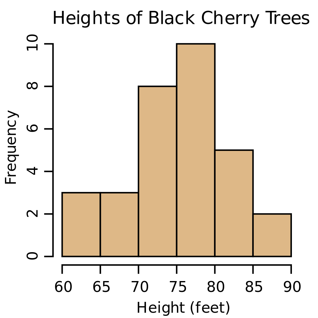
Before learning how to describe distributions, it’s obviously important to understand what they are. A distribution is the set of numbers observed from some measure that is taken. For example, the histogram below represents the distribution of observed heights of black cherry trees. Scores between 70-85 feet are the most common, while higher and lower scores are less common. The most commonly observed heights were between 75-80 feet, of which the researcher found 10 cases.

4 Key Concepts: a Preview

When describing distributions on the AP® Statistics exam, there are 4 key concepts that you need to touch on every time: center, shape, spread, and outliers. Below is a preview of the main elements you will use to describe each of these concepts. In the following sections, we’ll explain each of these terms one by one.

1. Center

a. Mean

b. Median

c. Mode

2. Shape

a. Symmetrical vs. Skewed

b. Unimodal vs. Bimodal

3. Spread

a. Range

b. IQR

4. Outliers

a. Are they any?

To ensure that you remember each of these 4 concepts, it is very helpful to come up with a mnemonic device, such as an acronym or a sentence. For example, you could rearrange the letters into SOCS, and remember to think, “When describing a distribution, ask about its ‘socks.’” Or, you could come up with a short sentence like Cats Sometimes Sleep Outside. If you make your own, it will be even easier to remember—the more unique and wacky, the better

1. Center

The first concept you should understand when it comes to describing distributions are the measures of central tendency: mean, median, and mode. There are multiple measures because there are different ways to think about what is the “center” of a distribution. Each measure has pros and cons and will be useful in different situations. As a result, you need to provide all three measures to give a full description.

Mean

The mean is the arithmetic average of all of the scores in your distribution. To calculate it, you simply add up all of the scores, and then divide by the total number of scores.

The mean is important for many other statistical calculations you will need in AP® Stats. However, the mean is also skewed by outliers. In other words, it is pulled towards the extremes.

Median

The median is the exact middle score in your distribution. To find the median, you must arrange all of the scores in numerical order. Then, you find the score that falls directly in the center, splitting the distribution evenly in half. If the number of scores in your distribution is even, there will be two scores in the center. In this case, you take the mean of the two middle numbers, and the result will be your median.

Mode

The mode is the easiest measure of central tendency to find. It is simply the most common score in your distribution, or the number that appears most often. Sometimes you may have a tie between two or more scores that all appear the same number of times in your distribution. In cases like this, you have more than one mode, and that is perfectly fine. However, there can only be one mean and one median per distribution.

2. Shape

The next thing to consider about a distribution is its shape. At the most basic level, distributions can be described as either symmetrical or skewed. You will see that there are also relationships between the shape of a distribution, and the positions of each measure of central tendency.

Symmetrical Distributions

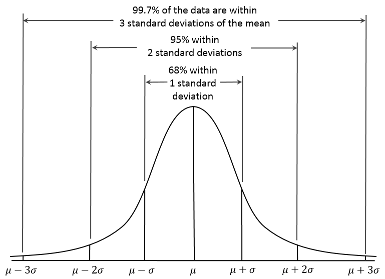
Symmetrical distributions are ones where the right and left halves are perfect mirrors of each other. Symmetrical distributions that are bell-shaped are also known as “normal distributions.” An example of a normal distribution is pictured below.

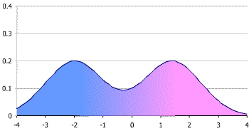
Distributions may also have a single peak or more than one peak. We call distributions with a single peak “unimodal.” “Modal” comes from the word “mode” – this makes sense when you consider that the peak of a distribution is also the score that appears most frequently. Distributions with two equal peaks are “bimodal” since two scores appear more frequently than the others but are equally frequent to each other. Below is an example of a bimodal distribution.

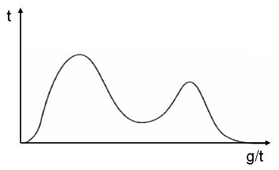
There are also cases in which a distribution appears to have two peaks, but one peak is larger than the other, such as the one below. For purposes of the AP® Statistics exam, these can be described as bimodal, though strictly speaking they are unimodal since there is only one most frequent score.

In normal distributions, the mean, median, and mode will all fall in the same location. If the distribution is symmetrical but has more than one peak, the mean and median will be the same as each other, but the mode will be different, and there will be more than one.

Skewed Distributions

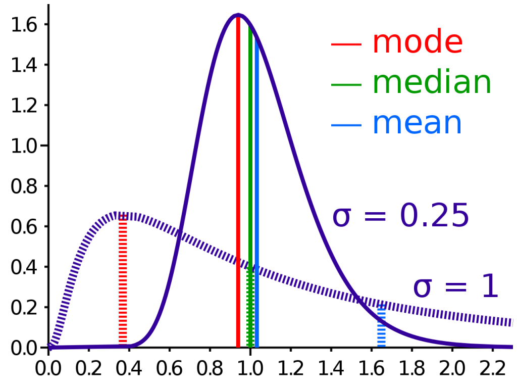
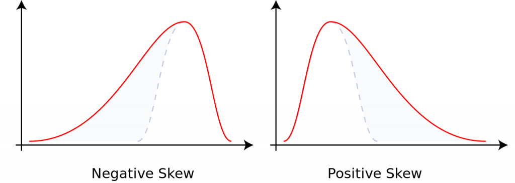
We call distributions that are not symmetrical “skewed.” They may be skewed either to the right or to the left. Right skew is also termed “positive skew,” since the x-axis becomes more positive as it moves to the right. As you might expect, left skew is termed “negative skew.”

The location of the “tail” determines the direction of the skew—the longer end of the distribution. If the tail is to the right, the distribution is right skewed, and vice versa. You can remember this by imagining taking a normal distribution, pinching one end of it, and stretching it out in that direction. The direction in which you stretch the distribution is the direction of the skew.

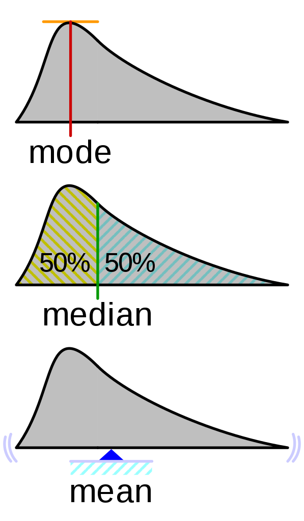
When a distribution is skewed, the mean will be pulled towards the tail. The halfway point of the distribution (the median) will also fall off the peak in the direction of the tail but not as far as the mean. The mode will remain at the peak. As a result, in a right skewed distribution the mode < median < mean, while in a left skewed distribution, the mean < median < mode. Understanding this idea can allow you to determine the shape of a distribution simply by knowing the measures of central tendency.

3. Spread

The main measure of spread that you should know for describing distributions on the AP® Statistics exam is the range. The range is simply the distance from the lowest score in your distribution to the highest score. To calculate the range, you just subtract the lower number from the higher one.

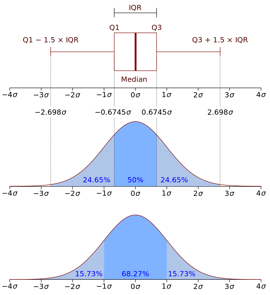
You can also utilize the interquartile range (IQR), which is a bit more complicated (for a review, see our other post on ranges). The IQR is the range of the middle 50% of the data. The IQR is useful for situations in which you have outliers.

4. Outliers

Outliers are scores that fall far outside of the main part of your distribution—either much higher or much lower. Outliers appear to be disconnected from the pack, meaning there are no scores observed between the outlier and the rest of the distribution. Below is an example of a distribution with one lower outlier. Notice on the right side, the distribution dips and rises again. However, this observation is not technically an outlier, since it is not disconnected from the rest of the distribution.

When describing distributions on the AP® Statistics exam, you simply need to indicate whether or not there are outliers, so this section of the question should be easy!

Practice Questions

Now that you know all of the concepts you need to describe a distribution on the AP® Statistics exam, let’s try a couple of practice problems!

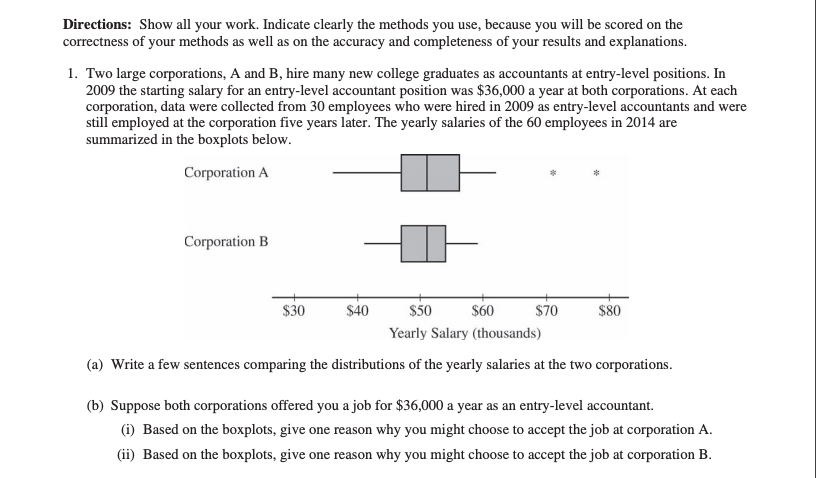
Practice 1 – 2015 AP® Statistics Free Response Question 1

Source: CollegeBoard

Now we just go through each of our 4 points!

Center: The median salaries for both corporations are approximately equal. (The mean and mode are not shown in boxplots, so we can’t touch on those here).

Shape: The salary distribution of corporation A appears skewed slightly to the left, while corporation B is approximately symmetrical.

Spread: The range and interquartile range for corporation A are larger than those of corporation B.

Outliers: Corporation A has two outliers, while corporation B has none.

Practice 2 – 2016 AP® Statistics Free Response Question 1

Source: CollegeBoard

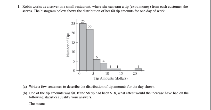
Center: The mode is the easiest measure to find since it is simply the most frequent score, which in this case is 0-2.5 dollars. You could also write all of the dollar amounts in a table to find the median and calculate the mean, but that would take more time and is unnecessary here. You know by the skew that the median is slightly higher than the mode, and the mean will be the highest of the three.

Shape: This distribution is unimodal and positively skewed.

Spread: We can’t find the exact range in this case since the graph shows us intervals of tip amounts rather than the exact numbers. However, the highest possible amount would be 22.5 dollars, and the lowest possible amount would be 0 dollars, making the greatest possible range 22.5 dollars. Using similar logic, we know that the smallest possible range is 17.5 dollars.

Outliers: This distribution has one outlier in the 20-22.5 dollars range.

Now that you’ve had a bit of practice, you should feel very comfortable using the 4 key concepts of center, shape, spread, and outliers. You’re ready to take on any question about describing distributions on the AP® Statistics exam!

Looking for AP® Statistics practice?

Check out our other articles on AP® Statistics.

You can also find thousands of practice questions on Albert.io. Albert.io lets you customize your learning experience to target practice where you need the most help. We’ll give you challenging practice questions to help you achieve mastery of the AP® Statistics.

Start practicing here.

Are you a teacher or administrator interested in boosting AP® Statistics student outcomes?

Learn more about our school licenses here.